On the instability of a nonlocal conservation law

Partial Differential Equations with nonlocal or fractional operators are widely used to model scientific problems in mechanics, physics, signal processing and other subjects, see for example [3] and references therein. We consider in this paper a nonlocal conservation law which appears in the formation and dynamics of sand structures such as dunes and ripples [7, 11]. Namely, Fowler ([7, 8, 9]) introduced the following equation

where $u=u(t,x)$ represents the dune height, $u_{0}\in L^{2}(\mathbb{R})$ is an initial condition, $T$ is any given positive time and $\mathcal{I}$ is a nonlocal operator defined as follows: for any Schwartz function $\varphi\in\mathcal{S}(\mathbb{R})$ and any $x\in\mathbb{R}$,

Equation (1) is valid for a river flow over an erodible bottom $u(t,x)$ with slow variation. The nonlocal term appears after a subtle modeling of the basal shear stress. This operator appears also in the work of Kouakou & Lagrée [10, 11].
The nonlocal term $\mathcal{I}$ can be seen as a fractional power of order $2/3$ of the Laplacian with the bad sign. Indeed, it has been proved [1]

where

with $a_{\mathcal{I}},b_{\mathcal{I}}$ positive constants and $\mathcal{F}$ denotes the Fourier transform. One simple way to establish this fact is the derivation of a new formula for the operator $\mathcal{I}$ [1]

with $C_{\mathcal{I}}=\frac{4}{9}$.
The operator $\mathcal{I}[u]$ is a weighted mean of second derivatives of $u$ with the bad sign and has therefore an anti-diffusive effect and creates instabilities which are controlled by the diffusive operator $-\partial_{xx}^{2}$. This remarkable feature enabled to apply this model for signal processing. Indeed, the diffusion is used to reduce the noise whereas the nonlocal anti-diffusion is used to enhance the contrast [3].

Recently, some results regarding this equation have been obtained, namely, existence of travelling-waves $u_{\phi}(t,x)=\phi(x-ct)$ where $\phi\in C^{1}_{b}(\mathbb{R})$ and $c\in\mathbb{R}$ represents wave velocity, the global well-posedness for $L^{2}$-initial data, the failure of the maximum principle, the local-in-time well-posedness in a subspace of $C^{1}_{b}$ [1, 2] and the global well-posedness in a $L^{2}$-neighbourhood of $C^{1}_{b}$, solving namely for $u=u_{\phi}+v$, with $v\in L^{2}(\mathbb{R})$ [4]. For this purpose, the following Cauchy problem solved by the perturbation $v$ has been considered:

where $v_{0}\in L^{2}(\mathbb{R})$ is an initial perturbation and $T$ is any given positive time.

Let us note also that any constant is solution of the Fowler equation. We shall prove below that these solutions are unstable.
To prove that a solution $u_{\phi}$ is unstable when $\phi$ is constant, we introduce the notion of mild solution (see Definition 1) based on Duhamel’s formula (8). We also give some numerical results that illustrate this fact.

The remaining of this paper is organized as follows: in the next section, we define the notion of mild solution and we give some results. Section 3 contains the proof of the instability. We introduce in section 4 an explicit finite difference scheme for which we give numerical simulations to illustrate the theory of the previous section.

The expression (8) is the Duhamel formula and is obtained using the spatial Fourier transform. The use of this formula allows to prove the local-in-time existence with the help of the contracting fixed point theorem. The global existence is obtained thanks to $L^{2}$ a priori estimate. We refer to [1, 4] for the proof.

In this section, we give the proof of the instability.

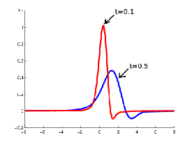
Let us first note that a fundamental property of the kernel $K$ is the non-positivity [1], see Figure 1. This feature enabled to prove the failure of the maximum principle. We use again this property to show that the constant solutions of the Fowler equation are unstable.

The spatial discretization is given by a set of points ${x_{j};j=1,...,N}$ and the discretization in time is represented by a sequence of times $t^{0}=0<...<t^{n}<...<T$. For the sake of simplicity we will assume constant step size $\delta x$ and $\delta t$ in space and time, respectively. The discrete solution at a point will be represented by $u^{n}_{j}\approx u(t^{n},x_{j})$. The schemes consist in computing approximate values $u^{n}_{j}$ of solution to (1) on $[n\delta t,(n+1)\delta t[\times[j\delta x,(j+1)\delta x[$ for $n\in\mathbb{N}$ and $j\in\mathbb{N}$ thanks to the following relation:

where $\mathcal{I}_{\delta x}$ is the discretization of the nonlocal term $\mathcal{I}$. We use a basic quadrature rule to approximate $\mathcal{I}$ given by (2)

Let us note that for compactly supported initial datum the sum is a finite sum. In this section, we want to simulate the instability stated previously. To this aim we must be careful to distinguish between the instability which stems from the model and numerical instabilities, which could be caused by a careless discretization.
The numerical stability ensures that the difference between the approximate solution and the exact solution remains bounded for increasing $t$ for $\delta x,\delta t$ given.

As noticed, the Fowler model amplifies slowly the low frequencies whereas the high frequencies are quickly dampened. Thus, the classical notion of $A$-stability (strong stability) and $C$-stability are not suitable nor desirable. A new definition of stability for this model has been considered in [5] and numerical stability criteria have been obtained.

In the following numerical test, we have to take care to choose $\delta x$ and $\delta t$ accurately following the stability condition, see [5]. We expose in Figure 3(a) the evolution of an initial flat bottom disturbed by a small bump for different times. As we can see the perturbation creates small ripples that grow with time without bound. This result proves that the perturbed solution goes away from the non-perturbed solution. This illustrates the instability of constant solutions for the Fowler model (1). Figure 3(b) shows the log-plot for the $L^{2}$-norm evolution of this perturbed bottom, which confirms the validity of the estimate given in Remark 2.

We thank Pascal Azerad and Clément Gallo for helpful comments. The author is supported by the ANR MATHOCEAN ANR-08-BLAN-0301-02

References

• [1] Alibaud N.; Azerad P.; D.Isebe ”A non-monotone nonlocal conservation law for dune morphodynamics ”, Differential and Integral Equations, 23 (2010), pp. 155-188.
• [2] Alvarez-Samaniego B.; Azerad P. ”Existence of travelling-wave and local well-posedness of the Fowler equation ”, Disc. Cont. Dyn. Syst., Ser. B, 12 (2009), pp. 671-692.
• [3] Azerad P.; Bouharguane A. ; Crouzet J.-F., Simultaneous denoising and enhancement of signals by a fractal conservation law, preprint: http://arxiv4.library.cornell.edu/abs/1004.5193.
• [4] Bouharguane A. , Global well-posedness and instability of a nonlocal conservation law , in preparation.
• [5] Azerad P.; Bouharguane A. , Finite difference schemes for a nonlocal conservation law, in preparation.
• [6] De Bouard A., Instability of stationary bubbles, SIAM J.Math Anal., 26 no. 3 (1995), pp. 566-582.
• [7] Fowler A.C., Dunes and drumlins, Geomorphological fluid mechanics, eds. A. Provenzale and N. Balmforth, Springer-Verlag, Berlin, 211 (2001), pp. 430-454.
• [8] Fowler A.C., Evolution equations for dunes and drumlins, Rev. R. Acad. de Cien, Serie A. Mat, 96 (3) (2002), pp. 377-387.
• [9] Fowler A.C, Mathematics and the environment, lecture notes http://www2.maths.ox.ac.uk/˜fowler/courses/mathenvo.html.
• [10] Kouakou K.K.J.; Lagrée P-Y, Evolution of a model dune in a shear flow, Eur. J. Mech. B Fluids, 25 no. 3 (2006), pp 348-359.
• [11] Lagree P-Y; Kouakou K. , Stability of an erodible bed in various shear flows, European Physical Journal B - Condensed matter, Vol. 47 (2005), pp 115-125.
• [12] Podlubny I., An introduction to fractional derivatives, fractional differential equations, to methods of their solution and some of their applications., Mathematics in Science and Engineering, 198 Academic Press, San Diego, (1999).