The Dirac-Moshinsky oscillator coupled to an external field and its connection to quantum optics
Abstract
The Dirac-Moshinsky oscillator is an elegant example of an
exactly solvable quantum relativistic model that
under certain circumstances can be mapped onto the Jaynes-Cummings model in quantum optics.
In this work we show, how to do this in detail. Then we extend it by considering its
coupling with an external (isospin) field and find the
conditions that maintain solvability.
We use this extended system to explore entanglement in relativistic systems and then
identify its quantum optical analog: two different atoms interacting with an electromagnetic mode.
We show different aspects of entanglement which gain relevance in this last system,
which can be used to emulate the former.
Keywords:
Dirac oscillator, Jaynes-Cummings model, entanglement.
PACS:
03.65.Pm, 03.67.Mn, 12.90.+b,
03.67.Bg, 03.65.Yz
1 Introduction
The fact that the Dirac equation is analytically solvable both for the free particle and the Coulomb problem made it plausible to look for other solvable Dirac systems whose non-relativistic counterparts, in analogy to the above, are superintegrable and/or algebraically solvable. Indeed additional problems are solvable in the relativistic setting; in particular, a generalization of the harmonic oscillator, with its large dynamical symmetry [1]. Moshinsky and Szczepaniak [2] did not only realize this, but constructed explicit solutions. This line was extensively followed by Moshinsky and his collaborators [2, 3].
We shall show that this solvability results from an additional conserved quantum number. This conservation indeed allows to preserve solvability in an algebraic sense even as we couple an additional isospin field into the system. Appropriate coupling conserves the quantum number and thus the symmetry of the extended problem. This solution was clarified by a mapping onto a more general problem in quantum optics, which we solved recently [4].
The connection to the quantum optics problem not only makes the solvability more understandable in a wider setting but also allows to conceive quantum optics experiments that emulate this system. Nowadays these experiments are feasible with trapped ions. The free particle Dirac equation has already been emulated [5, 6] and the mapping of the standard Dirac-Moshinsky oscillator (DMO) in dimensions on the Jaynes-Cummings model (JCM) has been proposed [7]. Here we shall review these methods and also show some cases in which the dimensional example can be mapped. We then propose a system of two atoms interacting with a cavity with different couplings on which the DMO coupled to an isospin field can in principle be realized.
The paper is organized as follows. In the section 2 we review and describe the Dirac-Moshinsky oscillator, in section 3 we present the Jaynes-Cummings model which is of great importance in quantum optics and cavity QED. In section 4 we describe how to map the relativistic model of the DMO onto the JCM for the three dimensional cases, this will allow us to formulate a straightforward method to extend the model as presented in section 5. In section 6 the quantum optical model related to the extended model will be presented.
2 The Dirac-Moshinsky oscillator
The DMO, introduced in 1989 by Marcos Moshinsky and A. Szczepaniak is a solvable quantum relativistic model which in the non-relativistic limit corresponds to the harmonic oscillator plus a spin-orbit coupling term. Noting that the momentum operator is linear in the Dirac equation, they proposed a linear term in position as well. We chose to write it as follows:
| (1) |
Here denotes the speed of light, and are the mass and frequency of the oscillator, and we make use of the following Dirac matrices:
| (2) |
We use two sets of Pauli matrices, namely for the spin of the particle and for the isospin. The representation of both and is the same, but we use different symbols to avoid confusion. We also use the convention of writing the isospin terms always at the left and in the following we shall omit to write the outer product explicitly to simplify notation.
Using the raising and lowering operators and the isospin states the state vector can be expressed as
| (3) |
and the Hamiltonian can be rewritten as
| (4) |
This form shows clearly the coupling between and , the big and small component of the state vector respectively. Squaring the Hamiltonian results in
| (5) |
where we have introduced the angular momentum operator . An analogous expression can be obtained for . At this point one can take the non relativistic limit noting that , with being the non-relativistic energy. The term at the left part becomes approximately , which means that is an eigenvalue of the operator at the right hand side which we recognize easily as the Hamiltonian of an isotropic harmonic oscillator plus a constant and a spin-orbit coupling term.
From equation (5) it is evident that commutes with (), the total angular momentum. For one has an additional constant of motion, that becomes clearer if one express the Hamiltonian in terms of the oscillator creation an annihilation operators and
| (6) |
where we have defined . This means that the eigenfunctions of can be expressed as expressed as a combination of , the isospin components, and , the eigenstates of harmonic oscillator coupled to spin . is the radial quantum number, is the angular momentum quantum number and its projection.
Before going into any further details of the DMO eigensystem, we take a short detour to introduce the quantum optical model related to our construction.
3 The Jaynes-Cummings model
The JCM [8] is a paradigm in quantum optics which can be thought of as a model that describes the interaction between a two level atom and one mode of the electromagnetic field, i. e. a cavity mode. The Hamiltonian describing such system can be written as
| (7) |
where and represent the creation and annihilation operator of photons in the cavity and are the raising and lowering operators of the atomic states. represents the coupling strength between the cavity and the atom and stands for the detuning of the atomic transition frequency from the cavity mode. The energy term of the mode is absent from (7), because it is written in the interaction picture.
To diagonalize the Hamiltonian (7) one notes that there is a conserved quantity which can be identified as the number of excitations in the system as there is only excitation exchange in the system. Using the basis , , where , are the ground and excited state of the atom and is a number state in the cavity, the Hamiltonian is block-diagonal in terms of matrices:
| (8) |
The eigenenergies can be easily obtained:
| (9) |
and one can find the corresponding eigenstates, which are known as dressed states in the literature:
| (10) |
with
| (11) |
Now that we have fixed the notation for the JCM and shown the simplicity of its solutions, we proceed to relate it with the DMO in the next section.
4 Mapping the DMO onto the JCM
In this section we describe the connection between the DMO and the JCM and show under which circumstances the DMO can be mapped onto the JCM.
4.1 DMO
Let us consider only one spatial dimension, namely the DMO. For this case one needs only two anticommuting Dirac matrices and we choose to write
| (12) |
where the superscript in the Hamiltonian indicates that we are working in the one-dimensional case. Using the creation and annihilation operators , and the raising and lowering operators of the Dirac Spinor one can rewrite the previous equation as
| (13) |
If one takes a look at equation (7), the connection in this case is obvious. This Hamiltonian is exactly the JCM Hamiltonian in quantum optics. Thus the DMO maps exactly onto the JCM, provided that one identifies , , the isospin with the atomic system and the spatial degrees of freedom with the cavity mode.
4.2 DMO
Now let us consider the case in two spatial dimensions, the DMO. For a full description of this case see [7, 9]. Here we need three anticommuting Dirac matrices and we choose
| (14) |
The ladder operators for each spatial dimension and can be used to construct a chiral representation in the form
| (15) |
which are also creation and annihilation operators with the canonical commutation rule and . Using the chiral ladder operators, together with the previously defined , one finds
| (16) |
The set of operators , is absent from equation (16), which means that the eigenstates of depend only on the number states , of the number operator , and are infinitely degenerate in the subspace spanned by . The connection to the JCM is also obvious. One has to identify the subspace of with the cavity mode, the isospin with the atomic system and in this case and .
4.3 3+1 DMO
Returning to the case described by the Hamiltonian in equation (6), one recognizes that is a conserved quantity. This tells us that a natural way of labeling the eigenstates of the total angular momentum and the 3D harmonic oscillator, is in terms of the oscillator quantum number . We define
| (17) |
There is no ambiguity in the previous definition if one remembers the dependence of on both and , the total angular momentum and radial oscillator quantum numbers. The key here is the parity of as there are two orthogonal states with the same value of and , in eq. (17), each one of these will be labeled by an with the same parity as . The lowest possible value will be .
In order to find the eigenstates of one has to know how the ladder operator , and its hermitian conjugates, act on the number states we just defined. We take the result from reference [1] and write it as
| (18) |
with
| (19) |
which takes into account the two separate cases, when has the parity of and . Using the basis where is diagonal, namely and , one can diagonalize the Hamiltonian in equation (6) in terms of matrices
| (20) |
In complete analogy with the JCM (see equation (8)) one can express the corresponding eigenergies in the following form:
| (21) |
The eigenstates will have the same functional form as the dressed states of the JCM in equation (10), but with the number states and energies .
The eigenstates with are infinitely degenerate as they have energies that do not depend on as can be seen from (21). In addition, the blocks in equation (20) have the same form to those of the JCM in equation (8). Therefore we can state that the infinitely degenerate part of the DMO can be mapped to the JCM, if one identifies and .
If one takes the degeneracy is finite. In this case the functional dependence of the blocks in equation (20) with is different to the JCM, so it can not be fully mapped. Even so, one could still emulate the finite degenerate part of the DMO in a JCM if one restricts only to one block of , here one should identify with .
5 A DMO coupled to an external field
Now we present the extension to the DMO interacting with an isospin field modeled as a potential that is summed to the total Hamiltonian
| (22) |
Among the many choices which preserve the integrability of the system, we use the simplest (i.e. linear) one by way of example, namely
| (23) |
Here represents the ladder operator for each dimensionality we considered in the previous section, and we have denoted with primes the isospin operator that acts on the field degrees of freedom. The full Hamiltonian is given by
| (24) |
For a physical discussion on and the covariant form of this system see [10].
We shall proceed from here taking as any ladder operator, that satisfies
| (25) |
Next we note that, due to the additional isospin, one has the integral of motion11 1 It will be further defined for each dimensionality considered
| (26) |
Using the basis where is diagonal, namely
| (27) |
the Hamiltonian is now block diagonal with its blocks given by the matrices
| (28) |
where depends on the dimensionality one choses.
The analysis in the previous section has allowed us to construct the generalization of DMO oscillator, in any of the three dimensionalities considered, coupled to an external isospin field. Table 1 shows for each dimensionality the correspondence of the ladder operator , the integral of motion , the quantum number and the function introduced in equation (28).
| DMO | Conserved quantum number | |||
|---|---|---|---|---|
The systems are again integrable and one can find the eigenenergies by diagonalizing each block . We shall not write the general solutions here as they can be found in [10]. Instead consider the evolution of a simple initial state and evaluate the entanglement of the DMO with the field.
5.1 Entanglement with the field
In this section we analyze the dynamical features of a Dirac particle under the influence of the external field. To this end and for simplicity, we use a product initial state formed by the lowest eigenstate of the DMO times the upper state of the field, namely
| (29) |
With our choice it follows from equation (27) that the basis is reduced to three states, because has to be non-negative. Thus the evolution will stay confined in a dimensional subspace22 2 For one would have dimensional subspaces. of the entire Hilbert space and the state vector at any time can be written as
| (30) |
If one simplifies things even more, by setting and one can find simple explicit solutions for these coefficients, namely
| (31) |
with the definitions
| (32) |

Our next task is to find the entanglement with the field. To this end one has to evaluate the reduced density matrix of the field by taking a partial trace over the DMO degrees of freedom. One finds the density matrix
The entanglement of the DMO with the field can be measured by the purity [11], obtained as
| (35) |
Figure 1 shows the purity of the field as a function of and , the field strength equal to the rest mass energy in this case. The purity starts at value as expected for an initial product state. Full entanglement of the isospin with the D occurs when purity reaches it minimum value of . Note that the oscillations between fully entangled and totally pure situations have a period which increases with . Normally one could expect an increase of the frequency with , but as already observed in [10], this is an effect of the resonance .
6 Two atoms inside a cavity
In this section we explain the connection of the coupled DMO of section 5 with quantum optical systems. The Hamiltonian in equation (24) can also be used in the context of quantum optics to describe a system composed of two atoms inside a cavity, provided one identifies with the ladder operator of the cavity and each isospin with an atom. Besides one has to regard and as the coupling of each atom to the cavity and and as the detuning of each transition level with the cavity mode.
This means that the extended model can also be mapped in cavity QED. Again the and cases can be mapped exactly, whereas the case can only be reproduced for the special situation considered in subsection 5.1, because in dimensions the coupling with the field mixes the dynamics of the infinitely degenerate part with the finitely degenerate part. This case in the blocks (28) of to depend on which changes by steps of as increases. For the equation (28) reduces to a matrix and only the value comes into play. Thus the particular case studied in subsection 5.1, which can represent the three dimensionalities, can be mapped to a quantum optical system. For this reason, in this work we focus only on the equivalent quantum optics model restricted to , that is an initially empty cavity.
In the context of quantum information theory, this is one of the simplest models which can be used in order to study two important aspects: entanglement and decoherence. The former is a resource for implementing quantum information protocols - and therefore, our ally - while the latter is an obstacle for such implementation. While these concepts play an important role in nurturing the quantumness of a central system, here we shall make use of quantum information measures as a tool to infer dynamical features of our problem in the simplest possible way.
We shall not rewrite the Hamiltonian as it is equal to the one in equation (24) and the same solutions apply. The initial state to consider here has to be different as the quantities of interest are others. We distinguish between the two atoms (central system) and the cavity (environment). So we shall begin with a product state of an atomic state times a number state of the cavity, and for simplicity we again take
| (36) |
note that for the state is exactly the same as in 29. We shall consider equivalent conditions as in subsection 5.1, which in this case means equal couplings to the cavity and atomic transition frequencies equally detuned from the cavity mode. With these considerations at time the state vector can be found in in a superposition like in equation (30), the only difference is that the coefficients will depend on , so we shall write them as
| (37) |
where and are given in equation (32) and we introduced
| (38) |
One has to remember that here represents the detuning of both atoms.
6.1 Entanglement measures
To evaluate the measures of entanglement one needs of the reduced density matrix of the two atoms, so we trace over the oscillator degrees of freedom to get:
| (39) |
To measure the entanglement between the two atoms (central system) and the cavity (environment) we use the purity and find
| (40) |
which serves as measure of the decoherence of the two atoms system.
To measure the entanglement between the atoms we use the concurrence [12] , where are the eigenvalues of in non-increasing order. In this case we find
| (41) |
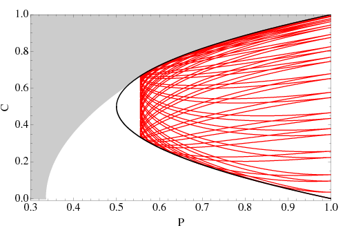
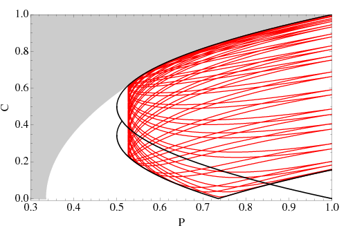
A useful way of visualizing both dynamics together is the so called plane [13, 4]. Figure 2 shows this plane for two separate cases, both with detuning . The left part shows in red for an initial state with , the equivalent case to subsection 5.1, whereas the right part shows it in red for . On both sides the red curves are parametrized up to . The black curve on both figures shows the behavior for zero detuning for and also on the right part for (lower black curve). Both figures show a gray area that correspond to states with density matrices which are not physically acceptable and its lower frontier corresponds to the maximally entangled mixed states.
It is interesting to note that in both cases the red curves form Lissajous like behavior in the plane. For zero detuning analytic expressions for the concurrence as a function of the purity can be found
| (42) |
these curves form the frontier of the region that the red curve partially fill as one can see in the figure 2. The region filled by the red curves reduces as one increases the detuning , that is the atoms feel less the effects of the cavity.
We also found similar behavior in [4] when instead we had zero detuning but interaction between the atoms.
7 Conclusions and final remarks
The Dirac Moshinsky oscillator in and dimensions was mapped to the Jaynes-Cummings model. For the case at least the infinitely degenerate part can be mapped. This scheme was based on explicitly using an invariant of these systems, which in the optical image acquires the simple meaning of the total number of excitations, which differs from the total energy because of detuning.
Based on this picture we obtained a soluble extension to the DMO coupled to an isospin field, if this coupling is carefully chosen to have an invariant that includes the excitations of the isospin field. The system not only retains solvability, but can be mapped to 2 atoms inside a cavity again for the and dimensional cases.
In the 2+1 dimensional DMO the presence of an external field which allows integrability does not break the infinite degeneracy. The absence of the operator for the JC model can be thought as ”inert” field modes which do not interact with the atoms in our system. In the quantum-optical system, other cavity modes may be populated by photons. However, if their frequencies are far off-resonance with our two-level atoms, the Hamiltonian in the interaction picture will contain no terms related to such modes. To complete the analogy, a Dirac particle in 2+1 dimensions contains such degrees of freedom, but they have no effect on the energies of the DMO.
We recognized that in our setting for dimensions, only the block can be represented by this diatomic model. However, the additional structure in the relativistic model may lead to other soluble models in atom optics, known or unknown at present. This will have to be the subject of further investigations.
By way of example we evaluated the purity of the field by tracing over the DMO degrees of freedom as well as other examples of the entanglement measures of the quantum optical system to which we mapped many of the discussed models.
References
- [1] M. Moshinsky and Y. Smirnov, The Harmonic Oscillator in Modern Physics , Hardwood Academic Publishers, Amsterdam, 1996.
- [2] M. Moshinsky and A. Szczepaniak, J. Phys. A 22, L817 (1989).
- [3] M. Moshinsky, et. al. The two body Dirac oscillator, AnniversaryVolume in Honor of J.J. Giambiagi, (World Scientific Press, Singapore, 1990). M. Moshinsky, et. al. Proceedings of the Rio de Janeiro International Workshop on Relativistic Aspects of Nuclear Physics, 271-307 (World Scientific, Singapore, 1990) M. Moshinsky, et. al. Proceedings of the 13th Oaxtepec Symposium on Nuclear Physics, Vol 13, No. 1 187-195 (1990). M. Moshinsky, et. al. Relativistic invariance of a many body system with a Dirac oscillator interaction, Lecture Notes in Physics, 1991, Volume 382 (1991).
- [4] J.M. Torres, E. Sadurni and T.H. Seligman, J. Phys. A 43 192002 (2010)
- [5] L. Lamata, J. Leon, T. Schaetz, E. Solano, Phys. Rev. Lett. 98, 253005 (2007).
- [6] R. Gerritsma, G. Kirchmair, F. Zähringer, E. Solano, R. Blatt, and C. F. Roos, Nature 463, 68 (2010).
- [7] Bermudez A, Martin-Delgado M A and Solano E 2007,Phys. Rev. A 76 041801.
- [8] Jaynes E T and Cummings F W 1963,Proc. IEEE 51 89.
- [9] A. Bermudez, M. A. Martin-Delgado, and A. Luis Phys. Rev. A 77 063815 (2008)
- [10] E. Sadurni, J.M. Torres and T.H. Seligman, J. Phys. A 43 285204 (2010)
- [11] M. Nielsen and I. Chuang Quantum Computation and Quantum Information , Cambridge University Press, Cambridge, 2000.
- [12] W. K. Wootters, Phys. Rev. Lett. 80, 2245 (1998).
- [13] M. Ziman and V. Bužek, Phys. Rev. A. 72, 052325 (2005).