Summing free unitary random matrices

The main objective of this paper is to begin investigating the following non–Hermitian random matrix model,

Here,

is a sum of $L\geq 2$ independent unitary random matrices of dimensions $N\times N$, weighted by some arbitrary complex numbers $w_{l}$, $l=1,2,\ldots,L$. Everywhere, except subsection III.2, the $\mathbf{U}_{l}$’s will belong to the simplest circular unitary ensemble (CUE). Moreover,

is a product of $K\geq 1$ complex random matrices, where $\mathbf{A}_{k}$, $k=1,2,\ldots,K$, is rectangular of dimensions $N_{k}\times N_{k+1}$ (hence, $\mathbf{P}$ has dimensions $N_{1}\times N_{K+1}$, and there must be $N=N_{1}$; the same are the dimensions of $\mathbf{W}$), and where all the real and imaginary parts of the matrix elements of the $\mathbf{A}_{k}$’s are independent random numbers with the Gaussian distribution of zero mean, i.e., concisely,

where the $\sigma_{k}$’s are real positive parameters (which set the respective variances to be $\sigma_{k}^{2}/(2(N_{k}N_{k+1})^{1/2})$). Finally, any matrix entry of any $\mathbf{U}_{l}$ is statistically independent from any entry of any $\mathbf{A}_{k}$.

In this article, I will consider only the part $\mathbf{S}$ (2), i.e., choose $K=0$. The more general model $\mathbf{W}$ (1) will be left for a separate paper.

The tools I apply — quaternion free probability, with its quaternion addition law (36) [1, 2], i.e., an extension of the standard free probability addition law (32) [3, 4] into the non–Hermitian realm — will allow to handle the above model only in the “thermodynamic limit,”

where the $K$ finite parameters $R_{k}$ are called the “rectangularity ratios.”

However, in subsection III.3, I will conjecture a finite–size modification of the results for the model $\mathbf{S}$ (with CUE’s as the summands), featuring a simple form–factor (67), which performs very well when numerically tested. The same form–factor should work for $\mathbf{W}$.

I will be interested in the two simplest statistical properties of the above model:

• •

  The mean density of the eigenvalues (“mean spectral density”) of $\mathbf{W}$ (in this paper, only of $\mathbf{S}$),

  $$\rho_{\mathbf{W}}(z,z^{*})\equiv\frac{1}{N}\sum_{i=1}^{N}\left\langle\delta^{(2)}\left(z-\lambda_{i}\right)\right\rangle.$$

  (6)

  There must be $N_{K+1}=N$ (i.e., $R_{1}=1$) for $\mathbf{W}$ to be a square matrix. Also, the averaging is performed with respect to the probability measure of $\mathbf{W}$, and the complex Dirac delta is used because the eigenvalues $\lambda_{i}$ are generically complex.

• •

  The mean density of the singular values, defined as the (real and non–negative) eigenvalues of the Hermitian random matrix $\mathbf{H}\equiv\mathbf{W}^{\dagger}\mathbf{W}$,

  $$\rho_{\mathbf{H}}(x)\equiv\frac{1}{N_{K+1}}\sum_{i=1}^{N_{K+1}}\left\langle\delta\left(x-\mu_{i}\right)\right\rangle.$$

  (7)

  (According to another terminology, these would be the singular values squared.) In this case $R_{1}$ can be arbitrary, and $\mathbf{H}$ has dimensions $N_{K+1}\times N_{K+1}$. The real Dirac delta is exploited since the singular values $\mu_{i}$ are real.

The model $\mathbf{W}$ (1) is interesting from the mathematical point of view, since it is non–Hermitian — and such random matrices have beautiful mathematical structure, more involved than Hermitian ones, plus multiple physical applications, ranging from finances and biology to quantum physics (for a review, consult e.g.,  [5]). In particular, the problems of summing (e.g.,  [6, 7, 8, 9, 10, 11, 12, 13, 14, 1, 2]) and multiplying (e.g.,  [15, 16, 17, 18, 19, 20, 21, 22, 23, 24, 25, 26, 27, 28, 29, 30, 31, 32, 14]) non–Hermitian random matrices have been drawing considerable attention — and the model $\mathbf{W}$ includes both these operations.

The model $\mathbf{W}$ (1) arises in the theory of random quantum states (see the textbook [33] and [34, 35] for review; I base this introduction on these latter works). Such objects are used for instance to describe states of a quantum system affected by noise, i.e., complicated interactions with an environment which can be regarded as random. Also, if one looks for generic properties of a complicated quantum state, one may assume it random. A random quantum state is defined by specifying a probability measure in the space of density matrices $\boldsymbol{\rho}$, i.e., Hermitian, weakly positive–definite (i.e., with non–negative eigenvalues) and normalized (i.e., $\textrm{Tr}\boldsymbol{\rho}=1$) matrices. One way to do this is to take any rectangular matrix model $\mathbf{X}$, and then $\boldsymbol{\rho}\equiv\mathbf{X}\mathbf{X}^{\dagger}/\textrm{Tr}(\mathbf{X}\mathbf{X}^{\dagger})$ is a proper random quantum density matrix.

More precisely, if one considers a bi–partite system consisting of a principal system $\mathcal{A}$ of size $N_{1}$ and an environment $\mathcal{B}$ of size $N_{2}$, one may form a pure state as a linear combination of the product basis,

Now, a mixed state on the principal system is obtained by taking the “partial trace” over the environment,

Then, different probability distributions of the pure states (i.e., of $\mathbf{X}$) lead to different ensembles of quantum density matrices.

The model $\mathbf{S}$ (2) thus appears in the following application of the above program: Consider a bi–partite system $(\mathcal{A},\mathcal{B})$ of size $N\times N$ (two “quNits”), and a maximally entangled state (the “generalized Bell state”) on it,

(A “typical” random state is entangled because there are much more entangled states than separable ones; the latter form a set of measure zero in the set of all states.) Now, perform on this state $L$ independent random local unitary transformations in the principal system $\mathcal{A}$,

the resulting states remain maximally entangled. Form a probability mixture of these $L$ states, i.e., a superposition with coefficients $w_{l}\in[0,1]$ such that $\sum_{l=1}^{L}w_{l}=1$, i.e.,

Finally, take the normalized partial trace over the environment $\mathcal{B}$, which leads to the random mixed state (9) with $\mathbf{X}=\mathbf{S}$.

The normalization, $\textrm{Tr}(\mathbf{S}\mathbf{S}^{\dagger})=N(\sum_{l=1}^{L}|w_{l}|^{2})+\ldots$, where the dots are $2\sum_{l<l^{\prime}}\textrm{Re}(w_{l}w_{l^{\prime}}^{*}\textrm{Tr}(\mathbf{U}_{l}\mathbf{U}_{l^{\prime}}^{\dagger}))\ll N$, if only the spectrum of the $\mathbf{U}_{l}$’s remains finite in the thermodynamic limit (5). Hence, it is enough to study the model $\mathbf{S}\mathbf{S}^{\dagger}$, or practically equivalently (modulo zero modes), $\mathbf{S}^{\dagger}\mathbf{S}$, i.e., the singular values of $\mathbf{S}$.

To my knowledge, the mean density of the singular values of $\mathbf{S}$ has been so far known only for all the $w_{l}$’s equal, which is the “Kesten distribution” [36]; the corresponding mean spectral density is also known [12, 13].

The model $\mathbf{P}$ (3) appears in another setup: Consider a system consisting of an even number $2K$ of subsystems, with the following sizes,

Consider an arbitrary product state $|\psi_{0}\rangle\equiv|0\rangle_{\mathcal{A}_{1}}\otimes|0\rangle_{\mathcal{A}_{2}}\otimes\ldots\otimes|0\rangle_{\mathcal{A}_{2K}}$. Now, form a random pure state by performing on $|\psi_{0}\rangle$ independent random local unitary transformations acting on the following pairs of the subsystems,

By definition, the result is a product state with respect to this latter pairing, i.e., it can be expanded in the product basis as

where the coefficients are collected into $K$ matrices $\mathbf{A}_{k}$ of rectangular dimensions $N_{k}\times N_{k+1}$. In the simplest case, they may be assumed Gaussian (4). Consider further the maximally entangled states (10) on the pairs $(\mathcal{A}_{2},\mathcal{A}_{3})$, …, $(\mathcal{A}_{2K-2},\mathcal{A}_{2K-1})$, and perform the projective measurement of $|\psi\rangle$ onto the product of these Bell states,

which yields a random pure state describing the remaining two subsystems, $\mathcal{A}_{1}$ and $\mathcal{A}_{2K}$,

As a final step, take the normalized partial trace over $\mathcal{A}_{2K}$, thus obtaining the mixed state on $\mathcal{A}_{1}$, (9) with $\mathbf{X}=\mathbf{P}$, whose statistical properties are directly related to the singular values of $\mathbf{P}$.

The mean density of the singular values of $\mathbf{P}$, with the assumption of all the sizes $N_{k}$ equal (i.e., all $R_{k}=1$ (5)), has been known as the “Fuss–Catalan distribution” [24, 32]; the corresponding mean spectral density has been found in [29]. For arbitrary $R_{k}$’s, after a primary work on the $K=2$ case [28], both mean densities have been derived in [30].

The model $\mathbf{W}$ (1) arises when a combination of both the above procedures is applied, i.e., one takes a probability mixture of $L$ random pure states defined on the $2K$ subsystems, performs the projective measurement on the product basis of the $(K-1)$ maximally entangled states, and takes the partial trace over the last subsystem.

According to my knowledge, the only known result concerns the mean density of the singular values of $\mathbf{W}$ for $L=2$, with equal weights, and $K=1$, which is the so–called “Bures distribution” [37, 38]. Therefore, generalization to arbitrary $L$, $K$, weights, as well as considering the eigenvalues — comprises an important research program, which will be accomplished in this and a forthcoming publication.

I will just mention that the model $\mathbf{S}$ (2), in the CUE case, finds applications to random walks on $L$–regular trees [36].

“Quaternion free probability” is a version of Voiculescu’s free probability calculus designed to handle non–Hermitian random matrices. To introduce it, let us however begin in the Hermitian realm. The “mean spectral density” of an $N\times N$ Hermitian random matrix $\mathbf{H}$ (7) is conveniently encoded in terms of the “holomorphic Green function,”

This is a meromorphic function, with poles coinciding with the mean (real) spectrum; in the large–$N$ limit, these poles coalesce into continuous intervals on the real axis, and this Green function turns into a holomorphic function on the whole complex plane except these cuts. The mean spectral density is retrieved from the holomorphic Green function taken in the vicinity of these cuts, through

as follows from the representation of the real Dirac delta, $\delta(\lambda)=-\frac{1}{2\pi\textrm{i}}\lim_{\epsilon\to 0^{+}}(\frac{1}{\lambda+\textrm{i}\epsilon}-\frac{1}{\lambda-\textrm{i}\epsilon})$; this is illustrated in figure 1. Remark that alternatively to the Green function, one often prefers the “holomorphic $M$–transform,”

For unitary matrices $\mathbf{U}$, the spectrum is not real, but is still one–dimensional (belongs to the centered unit circle $C(0,1)$, i.e., $\lambda_{i}=\textrm{e}^{\textrm{i}\theta_{i}}$, $\theta_{i}\in[0,2\pi)$), and the same formalism applies: The mean spectral density (in the variable $\theta\in[0,2\pi)$) can be generically expanded in the Fourier series, $\rho_{\mathbf{U}}(\theta)=\frac{1}{2\pi}(1+\sum_{n\geq 1}(m_{n}\textrm{e}^{-\textrm{i}n\theta}+m_{n}^{*}\textrm{e}^{\textrm{i}n\theta}))$, where the coefficients $m_{n}$ are called “moments.” (The inverse Fourier transform and triangle inequality imply $|m_{n}|\leq 1$.) Hence, the holomorphic Green function for $\mathbf{U}$,

where the positive moments are gathered into a generating function named the “holomorphic $M$–transform,”

For non–Hermitian random matrices $\mathbf{X}$, the approach must be altogether different because the eigenvalues are generically complex, and in the large–$N$ limit occupy on average some two–dimensional domain $\mathcal{D}$. The mean spectral density is now defined through the complex Dirac delta (6), whose representation $\delta^{(2)}(\lambda-\lambda_{i})=\frac{1}{\pi}\partial_{\lambda^{*}}\lim_{\epsilon\to 0}\frac{\lambda^{*}}{|\lambda|^{2}+\epsilon^{2}}$ is at the roots of the definition of the “non–holomorphic Green function” [39, 40, 41, 42, 43],

(with the convention for matrix division $\mathbf{A}/\mathbf{B}\equiv\mathbf{A}\mathbf{B}^{-1}$), since then the mean spectral density is obtained simply by taking a derivative,

(There are known intricacies concerning the order of limits in (23), but I will not be bothered by them.) An equivalent object, often handier, is the “non–holomorphic $M$–transform,”

The non–holomorphic Green function (23) is a more complicated object than the holomorphic counterpart (18) due to its denominator quadratic in $\mathbf{X}$. Hence, a linearizing procedure has been proposed [10] to introduce the “matrix–valued Green function,” which is a $2\times 2$ matrix function of a complex variable,

where

while bTr (“block–trace”) turns a $2N\times 2N$ matrix into a $2\times 2$ one by taking trace of its four $N\times N$ blocks,

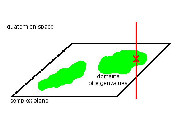
This need to leave the complex plane — into what we will see (paragraph II.2.3) is the quaternion space — is shown in figure 2. Now, (26) is already linear in $\mathbf{X}$, with the structure mimicking that of the holomorphic Green function (18). Its upper left element is precisely the non–holomorphic Green function (23), $[\mathcal{G}_{\mathbf{X}}(z,z^{*})]_{11}=G_{\mathbf{X}}(z,z^{*})$. Its lower right element carries no new information, $[\mathcal{G}_{\mathbf{X}}(z,z^{*})]_{22}=[\mathcal{G}_{\mathbf{X}}(z,z^{*})]_{11}^{*}$. Moreover, the negated product of the two off–diagonal elements (being a non–negative real number),

has been shown [44, 45] to describe correlations between left and right eigenvectors of $\mathbf{X}$ (a property I will not exploit), and also plays a role of an “order parameter”: it is positive inside the mean spectral domain $\mathcal{D}$ and zero outside of $\mathcal{D}$ (because $C_{\mathbf{X}}(z,z^{*})\propto\epsilon^{2}$, and the regulator $\epsilon$ can be set to zero outside of $\mathcal{D}$). From a practical point of view, once one finds $C_{\mathbf{X}}(z,z^{*})$ inside $\mathcal{D}$, then setting it to zero and solving for $z=x+\textrm{i}y$ yields an equation of the borderline $\partial\mathcal{D}$ in the Cartesian coordinates $(x,y)$.

In classical probability theory, if two random numbers $H_{1,2}$ are independent, then the PDF of their sum $(H_{1}+H_{2})$ is derived using the “classical addition algorithm”: First, the PDF’s of the constituents are encoded into the “characteristic functions,” $g_{H_{1,2}}(x)\equiv\langle\textrm{e}^{\textrm{i}xH_{1,2}}\rangle$, being complex functions of a real variable. Second, their logarithm is computed, $r_{H_{1,2}}(x)\equiv\log g_{H_{1,2}}(x)$. The independence property then ensures that this object simply adds when summing the random variables,

Third, exponentiating the result leads to the characteristic function, carrying the full spectral information, of the sum.

Free probability provides a similar algorithm for Hermitian random matrices: If $\mathbf{H}_{1,2}$ are free, then the mean spectral density of their sum $(\mathbf{H}_{1}+\mathbf{H}_{2})$ is calculated as follows: First, one needs to have the holomorphic Green functions (18) of the constituents. Second, one computes their “holomorphic Blue functions” [46], being functional inverses of the holomorphic Green functions,

The freeness property then implies that these Blue functions obey

Third, it remains to functionally invert the result to obtain the holomorphic Green function of the sum. (Let us mention that a more popular terminology is of the “$R$–transform,” $R_{\mathbf{H}}(z)\equiv B_{\mathbf{H}}(z)-1/z$, which is simply additive, $R_{\mathbf{H}_{1}+\mathbf{H}_{2}}(z)=R_{\mathbf{H}_{1}}(z)+R_{\mathbf{H}_{2}}(z)$.)

In [1, 2], a straightforward extension to the non–Hermitian world has been proposed. The procedure lies on the observation that the matrix–valued Green function (26) looks analogously to the holomorphic Green function (18) considered in the vicinity of the mean eigenvalue cuts, in the imaginary direction, i.e., $G_{\mathbf{H}}(\lambda+\textrm{i}\epsilon)$ — while in order to compute the holomorphic Blue function (31), the holomorphic Green function must be known on the whole complex plane. Therefore, the authors of [1, 2] felt compelled to replace the infinitesimally small regulator $\epsilon$ in (26) by an arbitrary complex number $d$ (actually, real and non–negative $d$ would be sufficient, since $\epsilon$ is real and non–negative),

(where $c$ is also an arbitrary complex number), thereby defining the “quaternion Green function” as a quaternion function of a quaternion variable,

(I will henceforth refer to $c$, $d$ and $a$, $b$ as to the “coefficients” of the respective quaternion.)

The “quaternion addition algorithm” has then been proven: Let $\mathbf{X}_{1,2}$ be free non–Hermitian random matrices. First, their quaternion Green functions (34) must be found (see subsection II.3 for how it is done in the case of Hermitian or unitary matrices). Second, these quaternion Green functions are to be functionally inverted in the quaternion space, leading to the “quaternion Blue functions,”

The freeness of the summands suffices to show that an analogue of (32) holds at the quaternion level,

Third, it is enough to functionally invert the result at the point $\mathcal{Z}_{\epsilon=0}$ to obtain the matrix–valued Green function (26) of the sum,

where $a=G_{\mathbf{X}_{1}+\mathbf{X}_{2}}(z,z^{*})$ and $|b|^{2}=C_{\mathbf{X}_{1}+\mathbf{X}_{2}}(z,z^{*})$. (The regulator $\epsilon$ may be set to zero here because it will be seen that the functional inversion to be performed in equation (37) takes care by itself of regulating the singularities at the eigenvalues: (37) will always yield a “holomorphic solution,” valid outside of $\mathcal{D}$, and a “non–holomorphic solution,” inside $\mathcal{D}$.)

There exists a special class of random matrices which permit an explicit calculation of the quaternion Green function (34) by means of a procedure called “rational Hermitization.” To describe it, perform the matrix inversion in (34), which gives the coefficients $a$, $b$ of the quaternion Green function through the coefficients $c$, $d$ of its argument,

Consider a symmetry constraint on $\mathbf{X}$ such that $\mathbf{X}^{\dagger}$ is a rational function of $\mathbf{X}$. Two primary examples are Hermitian ($\mathbf{H}^{\dagger}=\mathbf{H}$) and unitary ($\mathbf{U}^{\dagger}=\mathbf{U}^{-1}$) matrices. Then on the RHS of (38a)–(38b) one obtains rational functions of $\mathbf{X}$, which in turn may be expanded into simple fractions, and therefore written in terms of the holomorphic Green function (18) of $\mathbf{X}$. In other words, for this class of random matrices, knowing the holomorphic Green function is sufficient for knowing the (more complicated) quaternion Green function.

The rational Hermitization procedure for Hermitian matrices has been outlined in [1, 2] (it is needed e.g., when one adds a Hermitian to a non–Hermitian random matrix).

For an arbitrary unitary random matrix $w\mathbf{U}$ (where for further convenience I have included an arbitrary complex number $w$), one gets in this way the following coefficients of the quaternion Green function,

where $g\equiv\sqrt{((|c|-|w|)^{2}+|d|^{2})((|c|+|w|)^{2}+|d|^{2})}$ and $u\equiv\frac{1}{2w\overline{c}}(|w|^{2}+|c|^{2}+|d|^{2}+g)$, and recall the holomorphic $M$–transform of $\mathbf{U}$ (22).

In this case, equations (39a)–(39b) can be solved to provide the coefficients $c$, $d$ of the quaternion Blue function $\mathcal{B}_{w\mathbf{CUE}}(\mathcal{Q})$ through the coefficients $a$, $b$ of the quaternion $\mathcal{Q}$,

for some sign $s=\pm 1$.

For the sum (2) of the CUE’s with general weights $w_{l}$, the quaternion addition law (40) along with (37) yield equations for the coefficients $a$, $b$ of the matrix–valued Green function (26) of $\mathbf{S}$, i.e., $a=G_{\mathbf{S}}(z,z^{*})$ (or better (25), $M\equiv M_{\mathbf{S}}(z,z^{*})=za-1$) and $|b|^{2}=C_{\mathbf{S}}(z,z^{*})$,

where the $c_{l}$’s and $d_{l}$’s are given by (41a)–(41b).

This set (41a), (41b), (42a), (42b) can be easily simplified to the following form: $M$ is a solution to the equation

for some proper choice of the signs $s_{l}$ (yielding a meaningful solution), and then also

This is the master equation for summing free CUE random matrices.

Remark 1:

The master equation (43) and formula (44) may be cast in a more elegant way,

$$M=\sum_{l=1}^{L}M_{l},$$

(45)

where

	$\displaystyle-\frac{M(M+1)}{|z|^{2}}$	$\displaystyle=C,$		(46a)
	$\displaystyle-\frac{M_{l}(M_{l}+1)}{\left|w_{l}\right|^{2}}$	$\displaystyle=C,\quad l=1,2,\ldots,L,$		(46b)

where for short $C\equiv C_{\mathbf{S}}(z,z^{*})$. This form is surprisingly symmetric: Equation (46a) is identical as the set of definitions (46b) (cf. (72)–(73b)).

Remark 2:

The above set (45)–(46b) also provides an algorithm for rewriting it as a single polynomial equation for $M$: (1) Find $M_{L}$ from (45). (2) Substitute it to (46b), $l=L$. (3) Remove from it all the squares $M_{l}^{2}$, $l=1,\ldots,L-1$, by using (46b), $l=1,\ldots,L-1$. (4) Find from it $M_{L-1}$ (this requires solving a linear equation), and return to step (2), with $l=L-1$. The procedure ends at $M_{0}\equiv M$. One may also note that all the coefficients of the resulting polynomial equation are themselves symmetric polynomials in the $(L+1)$ arguments $|w_{l}|^{2}$, $l=0,1,\ldots,L$, where $w_{0}\equiv z$. However, in all the five examples presented below, it is better not to use this algorithm, but rather successively square the square roots in (43), as this leads to a polynomial equation of a lower order. For more general cases, however, the former algorithm seems inevitable.

Remark 3:

$M$ depends only on

$$R\equiv|z|,$$

(47)

i.e., the mean spectral density (24) is rotationally–symmetric around zero, and may be expressed as $\rho_{\mathbf{S}}(z,z^{*})=\frac{1}{\pi}\partial_{R^{2}}M$. Hence, we may focus on investigating just its radial part,

$$\rho^{\textrm{rad}}_{\mathbf{S}}(R)\equiv 2\pi R\left.\rho_{\mathbf{S}}(z,z^{*})\right|_{|z|=R}=\frac{\textrm{d}M}{\textrm{d}R}.$$

(48)

Remark 4:

Only the absolute values, and not the complex arguments, of the weights $w_{l}$ are relevant. Hence, it is enough to study real and positive weights.

Remark 5:

As explained at the end of paragraph II.1.3, once $C$ is found, then $C=0$ is the equation of the borderline $\partial\mathcal{D}$ of the mean spectral domain. According to (44) (or (46a)), this happens when $M=0$ or $M=-1$, i.e., in terms of the Green function (25), $G=1/z$ or $G=0$. This represents the matching on $\partial\mathcal{D}$ of the non–holomorphic quantities, valid inside $\mathcal{D}$ (i.e., $C$, $M$, $G$), with the holomorphic quantities, valid outside $\mathcal{D}$ (i.e., respectively, $0$, $0$ or $-1$, $1/z$ or $0$). This means that the mean spectral domain $\mathcal{D}$ is either (1) a centered disk, enclosed by the circle $R=R_{\textrm{ext}}$ — where the radius $R_{\textrm{ext}}$ is found by substituting $M=0$ to the master equation — or (2) a centered annulus, confined by an external circle $R=R_{\textrm{ext}}$ ($M=0$) and an internal one $R=R_{\textrm{int}}$ ($M=-1$). This is an instance of the “Feinberg–Zee single ring theorem” [8, 47, 48, 49], which states that if the mean spectral density is rotationally–symmetric around zero, then $\mathcal{D}$ is either a disk or an annulus.

I will now explicitly solve the master equation (43), or reduce it to a polynomial equation, in five cases.

As a first example of using the master equation (43), consider a sum of $L=2$ free CUE matrices, with arbitrary weights $w_{1,2}$. The master equation becomes linear, and yields the non–holomorphic solution,

Both holomorphic solutions, $M=0$ and $M=-1$, are compatible with (49), which implies that $\mathcal{D}$ is a centered annulus of radii,

(It becomes a disk only when $w_{1}=w_{2}$, see figure 4 (D).)

The radial mean spectral density of $\mathbf{S}$ follows by applying (48) to (49),

for $R_{\textrm{int}}\leq R\leq R_{\textrm{ext}}$, and zero otherwise. (The apparent singularities lie outside of the annulus.) I show the experimental eigenvalues on the complex plane and mark the theoretical annulus in figure 3. Formula (51) is numerically checked in figure 4 (A), finding perfect agreement in the bulk.

Consider now a sum of $L=3$ free CUE matrices, with arbitrary weights $w_{1,2,3}$. The master equation can be transformed into a fourth–order polynomial equation,

where the basis of the monomial symmetric polynomials,

where $p$ is a partition, $\textrm{Perm}(p)$ the set of all its permutations, $\textrm{Subs}(L,\#p)$ the set of all the $\#p$–element subsets of $\{1,\ldots,L\}$; also $v_{l}\equiv\sum_{k=1}^{L}(1-2\delta_{kl})|w_{k}|$.

Inserting $M=0$ or $M=-1$ into (52) leads to the values of the radii of the circles enclosing the mean spectral domain $\mathcal{D}$,

where $V_{l}\equiv\sum_{k=1}^{L}(1-2\delta_{kl})|w_{k}|^{2}$. One may check that the three numbers, $-V_{1,2,3}$, are either all negative or only one is positive; accordingly, $\mathcal{D}$ is a disk or an annulus.

I put forward a hypothesis that formulae analogous to (54a)–(54b) hold for arbitrary $L$.

The radial mean spectral density is given by (48) and equation (52), and is numerically verified in figure 4 (B), with excellent concord in the bulk.

Let now $L$ be arbitrary, but the weights assume only two values — let $L_{1}$ weights be equal to some $w_{1}$, and the other $L_{2}$ weights to some $w_{2}$ ($L_{1}+L_{2}=L$). The master equation can be transformed into a third–order polynomial equation,