Time-Changed Fast Mean-Reverting Stochastic Volatility Models
Abstract
We introduce a class of randomly time-changed fast mean-reverting stochastic volatility (TC-FMR-SV) models. Using spectral theory and singular perturbation techniques, we derive an approximation for the price of any European option in the TC-FMR-SV setting. Three examples of random time-changes are provided and are shown to induce distinct implied volatility surfaces. The key features of the TC-FMR-SV framework are that it is able to incorporate jumps into the price process of the underlying asset it allows for the leverage effect and it can accommodate multiple factors of volatility, which operate on different time-scales.
1 Introduction
Stochastic volatility models have played an important role in the derivatives markets over the past twenty years. Much of the success of stochastic volatility models is due to the fact that two of the earliest and most well-known models–the Heston model [19] and the Hull-White model [23]–capture the most salient features of the implied volatility surface while simultaneously preserving the analytic tractability needed to quickly calculate the price of an option. Yet the short-comings of these models is well-documented in literature. For example, the Heston model misprices far in- and out-of-the-money European options [11, 36].
There are a number of possible explanations for why the earliest stochastic volatility models fail to match implied volatility levels across all strikes and maturities. One theory is that a single factor of volatility, running on a single time scale, is not sufficient for describing the dynamics of the volatility process. Indeed, the existence of several factors of volatility has been documented in literature [2, 4, 8, 10, 15, 20, 25, 26, 28]. Such evidence has led to the development of multi-scale stochastic volatility models, i.e. models in which instantaneous volatility levels are controlled by multiple diffusions running of different time-scales [17, 13, 30].
Another line of reasoning states that jumps in the underlying asset price are required in order to capture the true dynamics of the market. Empirical work supports this notion [8]. Hence, academics and practitioners have developed models that incorporate both jumps in the asset price as well as stochastic volatility [5, 9, 34].
Along these lines, Mendoza-Arriaga et al. recently introduced a unified credit-equity framework in which the underlying asset is modeled as a stochastically time-changed scalar diffusion [27]. This work is notable for a number of reasons. First, the scalar diffusion that controls the asset price may exhibit both local volatility (i.e. volatility that is a function of the scalar diffusion itself) and killing (i.e. jump to default). When the local volatility is modeled as a negative power of the scalar diffusion a decrease in the underlying asset price results in an increase in volatility. This feature, known as the leverage effect, has been empirically documented [7]. Additionally, by subjecting the scalar diffusion to a random time-change the authors are able to incorporate jumps in the asset price as well as non-local factors of stochastic volatility. Finally, it is shown that, under relatively benign conditions, the framework of Mendoza-Arriaga et al. remains analytically tractable. We see great value in the work of Mendoza-Arriaga et al. and seek to build upon it.
In this paper, rather than base our model upon a scalar diffusion as in [27], we begin with the class of fast mean-reverting stochastic volatility (FMR-SV) models considered by Fouque et al. in [14]. Such models are important because they capture the empirically known-to-exist short time-scale of volatility [15, 21]. Additionally, FMR-SV models capture the leverage effect by negatively correlating the Brownian motions that drive the asset price and volatility processes. Using the methods outlined by Mendoza-Arriaga et al. in [27], we subject the FMR-SV class of models to a random time-change. For certain classes of time-changes this has the effect of adding jumps to the underlying asset price as well as additional factors of volatility. These additional factors of volatility operate on a different time-scale than the fast mean-reverting factor volatility. We refer to this class of models as the class of time-changed fast mean-reverting stochastic volatility (TC-FMR-SV) models.
The rest of this paper proceeds as follows. In section 2 we introduce the class of TC-FMR-SV models. This is done in a few steps. First, in section 2.1, we review the class of FMR-SV models considered in [14]. Next, in subsection 2.2, we explain how the FMR-SV class can be extended using random time-changes. Finally, in section 2.3, we review the three classes of random time-change. Some specific model assumptions are listed in section 2.4.
In section 3 we develop our option-pricing methodology. Again, this is done in several steps. First, in section 3.1 we review some important results from spectral theory, which we immediately apply to the European option-pricing problem in the TC-FMR-SV setting. This reduces the option-pricing problem to that of solving a single eigenvalue equation. In section 3.2, we find an approximate solution to this eigenvalue equation using techniques from singular perturbation theory. Then, in section 3.3 we show how to relate the approximate solution of the eigenvalue equation to the approximate price of a European option. The main result of our work is the formula we provide in Theorem 4 for the approximate price of a European option in the TC-FMR-SV setting.
2 Model Framework
In this section we introduce a class of TC-FMR-SV models. We begin by reviewing the FMR-SV class of models considered by Fouque et al in [14].
2.1 Review of FMR-SV Models
Under the physical measure the FMR-SV class of models has the following dynamics
| (1) | ||||||
| (2) | ||||||
| (3) | ||||||
| (4) | ||||||
Here, and are Brownian motions under with instantaneous correlation . The process represents the price of a non-dividend paying asset (stock, index, etc.), which has expected geometric growth rate and stochastic volatility . The process appears as an Ornstein-Uhlenbeck (OU) process with long-run mean and “vol of vol” . The OU process operates on time-scale , which is intended to be small so that the rate of mean-reversion of is high. It is in this sense that is fast mean-reverting. In fact, need not be an OU process specifically. The essential aspect of is that it be an ergodic process with a unique invariant distribution. The function is left unspecified, as only certain moments of play a role in the FMR-SV framework. Specific assumptions on the function and the process will be given in section 2.4. The parameter will play an important role throughout this paper. As such, we will use a superscript to indicate dependence on this small time-scale parameter.
For the purpose of option-pricing, it is necessary to move to the risk-neutral pricing measure, which we denote as . Under the FMR-SV class of models has the following dynamics
| (5) | ||||||
| (6) | ||||||
| (7) | ||||||
| (8) | ||||||
Here, and are Brownian motions under with instantaneous correlation . The Girsanov transformation, which relates the physical measure to the risk-neutral measure , is chosen such that the volatility-driving process acquires a market price of volatility risk and such that the discounted asset price is a martingale under . Note that is the risk-free rate of interest. As was the case with , the function is left unspecified, as only certain moments of play a role in the FMR-SV framework. Specific assumptions on will be given in section 2.4.
2.2 TC-FMR-SV Models
Under the risk-neutral measure , the TC-FMR-SV models have the following form
| (9) |
Here, is as described by equations (6) - (7) in section 2.1. The key difference between the TC-FMR-SV class of models and the FMR-SV class is that the dynamics of the of the discounted asset price , which would simply be given by the two-dimensional Markov diffusion in the FMR-SV framework, is now given by a time-changed diffusion . Broadly speaking, a random time-change is an increasing process, starting from zero, which is independent of and is right-continuous with left limits. We list specific assumptions on the random time-change in section 2.4.
2.3 Stochastic Time-Changes
In this paper, we will consider three classes of stochastic time-changes: Lévy subordinators, absolutely continuous time-changes, and time-changes that are the composition of a Lévy subordinator and an absolutely continuous time-change. These three classes of stochastic time-change are employed extensively in [27] in the context of local volatility models with state-dependent killing rates. Drawing inspiration from [27], we will use these classes of time-change in the context of FMR-SV models. A review of each of these classes is presented below. In an effort to avoid re-inventing the wheel, our discussion will be brief, focusing mainly on those aspects necessary for calculating option prices. For a more detailed discussion of stochastic time-changes, we refer the reader to [27].
2.3.1 Lévy Subordinator
A Lévy Subordinator is a non-decreasing Lévy process with positive jumps and non-negative drift. Because all Lévy processes have stationary and independent increments, the Laplace transform of a Lévy subordinator can be expressed as
| (10) | ||||
| (11) |
The function is known as the Lévy exponent of the subordinator and is given by the Lévy-Khintchine formula
| (12) |
Because all Lévy subordinators are of finite variation no truncation of integral (12) is necessary. The absence of a -independent constant term in (12) means that we have excluded any killing of the stochastic time-change. We require that the drift of the subordinator be non-negative .
The Lévy measure , which must satisfy
| (13) |
describes the arrival rate and distribution of jumps. Specifically, for some Borel set , the value gives the intensity of a Poisson process that counts the number of jumps of size .
For expectation (10) is always finite. However, in order to prove the accuracy of our pricing approximation in section 4, we will need to consider the case . To characterize the set , we recall Theorem of [33], where it is established that
| (14) |
In general, is an interval or where .
An important sub-class of Lévy subordinators are the subordinators of compound Poisson type. The jump component of such subordinators is described by a compound Poisson process with (net) jump arrival intensity and jump size distribution . For such subordinators, the Lévy measure can be written
| (15) |
in which case the Lévy exponent, given by equation (12), becomes
| (16) |
Although it is not strictly necessary for our framework, for the sake of computational simplicity, we will be primarily interested in Lévy subordinators for which the Lévy exponent is known in closed form.
We would like to emphasize the importance of Lévy subordinators as a class of stochastic time-change. Because Lévy subordinators exhibit jumps, the time-changed diffusion (and thus the asset price ) will exhibit jumps as well. To our knowledge, this is the first time that jumps in the asset price have been incorporated into the FMR-SV framework.
This concludes our brief review of Lévy subordinators. For more thorough coverage, we refer the reader to [6].
2.3.2 Absolutely Continuous Time-Change
We now consider stochastic time-changes of the absolutely continuous type. When we say is an absolutely continuous time-change we mean that can be written as
| (17) |
where is an infinite lifetime Markov process taking values in . The function shall be referred to as the rate function of stochastic time-change. We are primarily interested in absolutely continuous time-changes for which the Laplace transform
| (18) | |||||
| (19) | |||||
| (20) | |||||
is known explicitly. Here, the notation is used to indicate the conditional expectation . We note that (18) is always finite for . Values of for which (18) is finite depend on the specific choice of and must be checked on a case-by-case basis.
In the previous section, we showed that Lévy subordinators are an important class of stochastic time-change because jumps in the subordinator induce jumps in the asset price. Absolutely continuous time-changes are important for a very different reason; they have the ability to change a one-factor stochastic volatility model into a multi-factor stochastic volatility model. To see this, we define . Then, there exist -Brownian motions and with correlation such that [29]
| (21) | ||||||
| (22) |
Note that the volatility of is controlled by the product rather than just the single factor , which controls the volatility of . Note also that the multiple factors of volatility are operating on different time-scales; acts on a time-scale of and acts on a time-scale of . As demonstrated in [13], when compared to their one-factor counterparts, multi-factor stochastic volatility models in which the factors of volatility operate on different time-scales have the ability to vastly improve the fit to the empirically-observed implied volatility surface.
2.3.3 Composite Time-change
Finally, we may consider composite time-changes, which are time-changes of the form
| (23) |
Here, is a Lévy subordinator and is an absolutely continuous time-change, which is independent of . As long as the Lévy exponent of and the Laplace transform of are known explicitly, the Laplace transform of the composite time-change can be calculated as well. This is accomplished by conditioning on the absolutely continuous time-change as follows
| (24) | |||||
| (25) | |||||
| (26) | |||||
| (27) | |||||
Again, we remark that . However, values of for which depend on the specific choice of time-change .
The importance of composite time-changes is as follows: by combining a Lévy subordinator with an absolutely continuous time-change we are able to incorporate jumps in the asset price as well as add multiple factors of volatility to the class of FMR-SV models. The variety gained by combining different types of stochastic time-changes provides us with considerable modeling flexibility.
Remark on Notation
Throughout this paper we shall use the superscripts to specify which type of random time-change we wish to consider. The notation will be used to denote a Lévy subordinator, the notation will be used to denote an absolutely continuous time-change and the notation will be used to denote a composite time-change. Finally, if we do not wish to specify a particular class of random time-change we will omit the superscript altogether and use the notation .
2.4 Specific Model Assumptions
We have now described the TC-FMR-SV class of models. However, we have not been specific about certain technical assumptions on the process , the functions and and the stochastic time-change . The purpose of this section is to list these assumptions in one place. Our assumptions are as follows:
- 1.
Under the physical measure , the process is ergodic and has a unique invariant distribution , which is independent of . We note that this implies the moments are uniformly bounded in . That is, for every there exists a positive constant such that
(28) - 2.
- 3.
- 4.
The random time-change is a strictly increasing càdlàg process, which is independent of and satisfies and
(29)
2.5 The Martingale Condition
Although we specified the class of TC-FMR-SV models under a supposedly risk-neutral measure , we have not yet shown that the non-dividend-paying asset in these models satisfies the martingale condition
| (30) |
which is required in order for to actually be risk-neutral. In fact, because , and are time-homogeneous Markov processes, as rigorously established in [27], the martingale condition reduces to
| (31) |
where we have used the short-hand notation to denote the conditional expectation . We can verify equation (31) by conditioning on the random time-change as follows
| (32) | ||||
| (33) | ||||
| (34) |
where we have used the fact that is an exponential martingale. Having established that the discounted stock-price process is a martingale under in the TC-FMR-SV framework, we now move on to the option-pricing problem.
3 Option Pricing
In this section, we discuss how the approximate price of any European option can be calculated in the TC-FMR-SV setting.
3.1 Spectral Representation of European Option Prices
We begin with a brief review of some important results from spectral theory and semigroup operators.
Theorem 1.
Suppose is a self-adjoint operator acting on a Hilbert space . Consider the eigenvalue equation for
| (35) |
We denote by the projection-valued spectral measure of and by the spectrum of . Then:
- 1.
The operator has the following spectral representation
(36) If is a real-valued Borel function on , then can be defined via operational calculus and is given by
(37) - 2.
If there exists a number such that for all , then
(38) defines a strongly continuous one-parameter semigroup and the solution to the Cauchy problem
(39) is given by
(40)
Proof.
For convenience, we will write (40) as
| (41) |
where . This will help to make it clear that is a projection of onto the eigenspace . In the special case when the spectrum is purely absolutely continuous with respect to the Lebesgue measure, equation (41) can be written
| (42) |
where the are constants chosen such that .
Now, consider a function , defined as
| (43) |
The backward variables satisfy the Kolmogorov backward equation
| (44) | ||||
| (45) |
Note that the term carries a minus sign because is a forward variable. We use the notation to indicate the infinitesimal generator of the Markov process , defined in (6) - (7). For clarity, we write explicitly and state its domain
| (46) | ||||
| (47) | ||||
| (48) |
Now, suppose we have the solution to the following eigenvalue equation
| (49) |
By, solution to the eigenvalue equation we mean that we have the full set of eigenvalues and corresponding eigenfunctions for which (49) holds. Then if the operator were self-adjoint on some Hilbert space , by Theorem 1, the solution to Cauchy problem (44) - (45) could be expressed as
| (50) |
where the measure would be determined by BC (45).
It is not apparent that there exists a Hilbert space on which is self-adjoint. As such, it is not clear at this point that eigenvalue equation (49) has a solution, nor is it clear that has a representation of the form (50). Nevertheless, in this paper we do not endeavor to solve the full the eigenvalue equation (49). Rather, we shall use techniques from singular perturbation theory to find an approximate solution to (49). We will show that the operator associated with the lowest order solution to (49) is in fact self-adjoint on some Hilbert space. As a result, can be approximated by a function of the form (50). For the moment, however, it will ease our calculations if we assume that can be written as (50), which we shall refer to as the spectral representation of .
Supposing can be approximated by a function of the form (50), we would like to use this knowledge to find a spectral representation for the price of a European option in the TC-FMR-SV framework. To this end, we consider a European option with payoff at maturity date . Using risk-neutral pricing, and the Markov property of , we may write the price of a European option as
| (51) |
Conditioning on the random time-change we find
| (52) |
Note that is just a parameter here–not a variable of . Now, we use (50) to replace with its spectral representation. We have
| (53) | ||||
| (54) |
where passing the expectation through the integral is allowed by Fubini’s theorem. We have used the notation to remind us that depends on the paramter through the BC . Assuming it exists, we refer to (54) as the spectral representation of the option price . Note that the expectation is given explicitly by either (10), (18) or (26), depending on the type of random time-change. Hence, in order to fully specify the price of the option , what remains is to solve eigenvalue equation (49) and determine the measure from the BC
| (55) |
3.2 Asymptotic Analysis of the Eigenvalue Equation
For general and there is no analytic solution to the eigenvalue equation . However, we note that can be conveniently decomposed in powers of as
| (56) | ||||
| (57) | ||||
| (58) | ||||
| (59) |
This decomposition suggests a singular perturbative approach. To this end, we expand and in powers of . We have
| (60) | ||||
| (61) |
Expanding in powers of (rather than some other power of ) is a natural choice given the form of . The validity of this expansion will be justified in section 4, when we establish the accuracy of our pricing approximation.
We now insert the expansions for and into eigenvalue equation (49) and collect terms of like-powers of . The and equations are
| (62) | ||||||
| (63) |
Noting that all terms in and take derivatives with respect to , we may (and do) choose solutions of the form and (i.e. functions of only). Continuing the asymptotic analysis, the order and equations are
| (64) | ||||||
| (65) |
where we have used in (64). Equations (64) and (65), respectively, are Poisson equations for and in the variable of the form
| (66) |
where is the infinitesimal generator of under the physical measure . We wish to consider only those solutions of (66) that exhibit at most polynomial growth as . With this restriction, a necessary condition for the solvability of (66) is
| (67) |
We remind the reader that is the invariant distribution of under the physical measure . Equation (67) is referred to as the centering condition. Please refer to Appendix A for a treatise on the Poisson equation and the centering condition. Throughout this paper, the notation will always indicate averaging with respect to the invariant distribution . In equations (64) and (65) the centering conditions become
| (68) | ||||
| (69) |
Eigenvalue equation (68) can be solved explicitly, as the operator is given by
| (70) |
However, in order to solve equation (69), we need an expression for . To this end, we note from (64)
| (71) |
Now, introducing as a solution to the following Poisson equation 11 1 We note that (72) satisfies the centering condition and exists by assumption 2c of section 2.4.
| (72) |
we may express as
| (73) |
where is some function which is independent of . Hence, using (58) we find that is given by
| (74) | ||||
| (75) |
where
| (76) |
Thus, from (69) we have
| (77) |
Given a solution to (68), one can use (77) to find expressions for and .
This concludes our asymptotic analysis of eigenvalue equation (49). Before we present an explicit solution to (68) and (77), we recall the following result from Sturm-Liouville theory.
Theorem 2.
The eigenfunctions of equation (68) form a complete orthonormal basis in the Hilbert space where
| (78) |
The notation indicates the complex conjugate of .
Proof.
Theorem 3.
The order eigenfunctions and eigenvalues are given by
| (79) | ||||
| (80) |
where . The order corrections and are
| (81) | ||||
| (82) |
where and are defined in (76). We note that .
3.3 Option Prices
We have found explicit expressions for the approximate eigenvalues and approximate eigenfunctions . We now use these expressions to specify the approximate price of an option. The following Theorem serves as the main result of our work.
Theorem 4.
The approximate price of an option is given by
| (84) | ||||
| (85) | ||||
| (86) |
where the coefficients are given by
| (87) |
For a composite time-change we have
| (88) | ||||
| (89) | ||||
| (90) | ||||
| (91) |
The corresponding expressions for a Lévy subordinator and an absolutely continuous time-change can be recovered by setting and respectively. The eigenfunctions and the approximate eigenvalues are given in Theorem 3.
Proof.
Consider the spectral representation of given by (50). Recall that we use the notation to remind us that has a BC that takes as a parameter. We expand and in powers of
| (92) | ||||
| (93) |
Note that we have expanded the measure in terms of a density as the spectrum of the eigenvalue problem is absolutely continuous with respect to the Lebesgue measure . Inserting expansions (60), (92) and (93) into (50) and collecting terms of like-powers of yields
| (94) | ||||||
| (95) |
where we have dropped the term because . Expressions for and can be obtained from the BC’s and . We have
| (96) | ||||||
| (97) |
Hence
| (98) | ||||||
| (99) |
where we have used (83).
We have now obtained an explicit expression for . In order to find an expression for the approximate price of an option we simply insert our expansion for into (52), which yields (85) and (86). Expressions (88) and (89) are given for a composite time-change and can be obtained by expanding in powers of . ∎
Remark.
Corollary 5.
The function is linear in the group parameters
| (100) |
Proof.
Corollary 5 relates to a very important feature of the TC-FMR-SV pricing methodology. Consider first the FMR-SV framework (no time-change). To describe a particular model within the FMR-SV class, one would have to specify an ergodic diffusion , a market price of volatility risk and a volatility function . For the purposes of illustration, we chose to specify as an OU process. This choice led us to introduce five unobservable parameters (, , , , ). Note however, that neither the value of these parameters nor the precise form of and are required in order to calculate the approximate price of an option (the approximate price of an option in the FMR-SV framework is given by setting in the TC-FMR-SV framework). Rather, to , the approximate price of an option can be expressed in terms of as well as the observable parameters .
As mentioned previously, the particular choice of as an OU is not central to our analysis. We could have simply written under the physical measure as
| (101) |
where and are such that the assumptions of section 2.4 are satisfied. In this case, the group parameters would have become
| (102) |
The key point is that, when the volatility-driving process is fast mean-reverting and satisfies the conditions of section 2.4, the details of the process are unimportant. In terms of option-pricing, to , all that matters are the values of . This is true regardless of the particular choice of .
In the TC-FMR-SV framework the situation remains the same – to calculate the approximate price of an option, precise knowledge of the volatility-driving process is not required. However, the particular choice of random time-change does affect the approximate price of an option. Thus, when calibrating a particular model within the TC-FMR-SV class to fit market data (be the data quoted option prices or implied volatilities), the unobservable parameters that must be extracted are as well as the parameters of the random time-change . We will show in section 5 that different time-changes induce distinct implied volatility surfaces. Whether the introduction of time-change parameters is justified by the modeling flexibility the random time-change provides is a topic left for future research.
4 Accuracy of the Approximation
In the previous section, we gave a derivation of the approximate price of a European option using singular perturbative arguments. The purpose of this section is to establish the accuracy of this approximation. In addition to the assumptions listed in section 2.4, we shall need one additional assumption for our accuracy proof.
- •
The payoff function and all derivatives taken with respect to are smooth and bounded.
Obviously, the most common options – calls and puts – do not fit this assumption. To prove the accuracy of our pricing approximation for calls and puts would require regularizing the option payoff as was done for the class of FMR-SV models in [16]. The regularization procedure is beyond the scope of this paper. As such, we limit our analysis to options with smooth and bounded payoffs.
Before stating our main accuracy result we need the following Lemma.
Lemma 6.
Suppose is at most polynomially growing. Then, there exists a constant such that
| (103) |
Proof.
First, we define , the exponential martingale used in Girsanov’s theorem to transform the measure on from to
| (104) |
We note
| (105) | ||||
| (106) | ||||
| (107) | ||||
| (108) |
where we have used assumption 3b of section 2.4 to bound by . Hence
| (109) |
The first inequality is an application of Cauchy-Schwarz. The second inequality follows from the above bound as well as assumption 1 of section 2.4. Since is bounded by a polynomial, this proves lemma 6. ∎
From here, we shall proceed as follows. First, we shall establish the accuracy of the approximation . Then, we show how this result can be related to the accuracy of the approximate option price .
Theorem 7.
Proof.
First, we define a remainder term
| (111) |
Next, we see that
| (112) | ||||
| (113) | ||||
| (114) | ||||
| (115) | ||||
| (116) | ||||
| (117) | ||||
| (118) | ||||
| (119) |
Now, from the Feynman-Kac formula we note that , which is the solution to PDE (116) with BC (118), has the following stochastic representation:
| (120) |
As established in [14], from the boundedness of the payoff function , and from the assumptions of section 2.4, one can deduce that and are bounded in and at most polynomially growing in . Hence, by lemma 6, there exists a constant such that
| (121) |
Therefore,
| (122) | ||||
| (123) | ||||
| (124) | ||||
| (125) |
for some constants and . This establishes Theorem 7. ∎
Now we state our main accuracy result.
Theorem 8.
For fixed there exists a constant such that for any the price of a European option given by (52), satisfies
| (126) |
Proof.
| (127) | ||||
| (128) | ||||
| (129) | ||||
| (130) | ||||
| (131) | ||||
| (132) | ||||
| (133) |
for some constants and . This establishes Theorem 8. ∎
5 Call Option Examples
In this section we provide examples of how to calculate the price of a European call option in four different time-change regimes. These examples demonstrate both the flexibility and analytic tractability of the TC-FMR-SV framework.
5.1 FMR-SV
The first regime we consider is that of no random time-change (i.e. ). This choice for reduces the TC-FMR-SV framework to that of pure FMR-SV. To calculate the approximate price of a European call option we use equations (85) and (86) of Theorem 4. Since is not random in the present scenario, expectations (88) and (89) reduce to
| (134) |
The eigenfunctions are given in (79). Expressions for and can be found in (80) and (82) respectively. Hence, what remains in order to calculate the approximate price of a call option is an expression for .
For a European call with strike price and time of maturity , the option payoff is given by
| (135) |
Using equation (87) we calculate
| (136) | ||||
| (137) | ||||
| (138) |
Note that integral (137) will not converge for purely real values of . However if we move into the complex plane and we fix the imaginary part of such that , then integral (137) will converge. Upon doing this, when calculating option prices using (85) and (86), we must remember to hold the imaginary part fixed and integrate with respect to the real part of (i.e. set ).
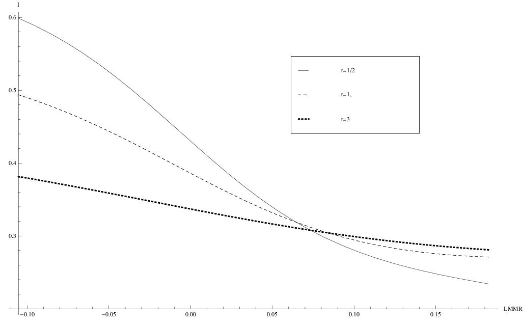
Figure 1 demonstrates the implied volatility surface induced by the TC-FMR-SV framework in the regime. We plot implied volatilities versus -moneyness-to-maturity ratio (LMMR). We remind the reader that and LMMR are defined by
| (139) | ||||
| LMMR | (140) |
where is the Black-Scholes price of a call option with strike price , time to maturity and volatility . The notation is used here to indicate the approximate price of call option as calculated in the TC-FMR-SV framework with strike price and time to maturity . The parameters used in figure 1 are
| (141) |
We note that the volatility surface induced by the regime is able to produce a negative at-the-money (ATM) skew, which is typical of equity call options. However, without a stochastic time-change, the implied volatility surface will not exhibit a smile [14].
5.2 TC-FMR-SV: Lévy Subordinator
Next, we consider a regime where the random time-change is given by a Lévy subordinator. The jumps of our prototype Lévy subordinator will be modeled as a compound Poisson process. Specifically, we consider
| (142) |
where is the drift of the Lévy subordinator, is a homogeneous Poisson process with jump-arrival intensity and the are i.i.d. random variables with exponential distribution and mean . As noted in section 2.3.1 the Lévy measure of a compound Poisson process can be written as the product of the (net) jump-arrival intensity and the distribution of the i.i.d. jumps. In this case
| (143) |
Using equations (16) and (143), we calculate the Lévy exponent of a as
| (144) |
For a Lévy subordinator expectations (88) and (89) reduce to
| (145) |
where, for a compound Poisson process with exponentially distributed jumps, and are given by
| (146) |
The coefficients , given by (138), are unaffected by the choice of random time-change. Hence, the approximate price of a European call option can now be calculated using (85) and (86).
Figure 2 plots implied volatilities versus LMMR in the TC-FMR-SV regime in which is given by (142). The parameters used in figure 2 are
| (147) |
We note that the implied volatility surface of figure 2 exhibits an ATM skew as well as a true smile with implied volatilities rising at the largest strikes. The strong skew and smile are particularly noticeable at shorter maturities. This is consistent with the findings of [18], where it was noticed that a model for the underlying asset must contain jumps in order for the induced implied volatility surface to capture the steep skew and strong smile of the empirically observed implied volatility surface for short-maturity options.
5.3 TC-FMR-SV: Absolutely Continuous Time-Change
Recall that an absolutely continuous time-change is of the form (17). As an example, we consider to be the classic Cox-Ingersoll-Ross (CIR) process and the rate function to be the identity . We have
| (148) | ||||
| (149) |
where is a Brownian motion under . Here is the rate of mean-reversion of the CIR process and is the long-run mean. We shall refer to as the “vol of vol” since controls the volatility of , which in turn contributes to the volatility of . We shall enforce the condition so that the CIR process remains strictly positive for all time (see [24], Chapter 6).
In order to compute option prices in the absolutely continuous time-change regime, we need to know the Laplace transform of . This is a classical calculation, which can be found in [24]. Here, we simply state the result
| (150) | ||||||
| (151) | ||||||
| (152) | ||||||
| (153) | ||||||
| (154) | ||||||
For an absolutely continuous time-change , expectations (88) and (89) reduce to
| (155) |
The above expectations, along with expression (138) for , are enough to calculate the approximate price of a call option using (85) and (86).
Figure 3 plots implied volatilities versus LMMR in the TC-FMR-SV regime in which is given by (149). The parameters used in figure 3 are
| (156) |
We observe that the implied volatility surface in figure 3 exhibits an ATM skew as well as a slight smile effect. Though, neither the skew nor smile in figure 3 is as pronounced as in figure 2 where the stochastic time-change is given by a Lévy subordinator .
5.4 TC-FMR-SV: Composite Time-Change
6 Summary and Conclusions
In this paper we introduce a class of TC-FMR-SV models. The key features of our modeling framework are:
- 1.
We are able to include jumps in the price process of the underlying asset.
- 2.
We can incorporate multiple factors of stochastic volatility, which run on different time scales.
- 3.
We are able to account for the empirically observed negative correlation between asset returns and volatility (the leverage effect).
Some of the main results of our analysis are:
- 1.
We provide simple formulas to calculate the approximate price of any European option.
- 2.
By combining different time-changes, we are able to produce a wide array of implied volatility surfaces.
Overall, we feel that the flexibility provided by the TC-FMR-SV framework and the analytic tractability it provides, merit continued research in this area. A logical next step, for example, would be to incorporate default of the underlying asset into our class of models, as done in [27]. Additionally, characterization of the implied volatility surface through an expansion would be useful.
Thanks
The authors of this paper would like to thank Jean-Pierre Fouque and two anonymous referees for their thoughtful comments on this work. Their suggestions have greatly improved both the quality and readability of this paper.
Appendix A Poisson Equations and the Fredholm Alternative
The purpose of this appendix is to explain why centering condition (67) is necessary in order for the Poisson equation (66) to admit a solution. To begin, we consider an ergodic Markov diffusion that lives on , has invariant distribution and whose infinitesimal generator and adjoint are given by
| (159) |
From the Kolmogorov forward equation, the density satisfies and is given by
| (160) |
where is a constant such that .
We consider the following Poisson problem: find such that
| (161) | ||||||
| (162) |
Multiplying by and integrating with respect to we find
| (163) | ||||
| (164) |
where we have used integration by parts and . Hence,
| (165) |
In section 3.2 we considered Poisson equations with respect to the operator , the infinitesimal generator of the volatility-driving process under the physical measure , which we chose to be an OU process. Under the physical measure the OU process has an invariant distribution . In this setting, in equation (165) asymptotically behaves like . Thus, if we restrict ourselves to solutions of (161) that have at most polynomial growth as then the right-hand side of (165) is zero. Hence, a necessary condition for the solvability of (161) becomes , which is precisely the centering condition given in (67).
We have established that is a necessary condition for the solvability of (161). It turns out is also a sufficient condition for (161) to have a solution. The Fredholm alternative states that one of the following is true:
- 1.
has a unique solution (i.e. is invertible) or
- 2.
has a non-trivial solution, in which case has a solution if .
For the OU process with infinitesimal generator , we note that has a non-trivial solution – namely . Hence by the Fredholm alternative has a solution if . Since we have , the statement is equivalent to the centering condition . The following (formal) solution can easily be checked
| (166) |
We refer the reader to section of [12] for a detailed exposition on Poisson equations and the Fredholm alternative.



References
- [1] M. Al-Gwaiz, Sturm-Liouville theory and its applications, Springer Verlag, 2008.
- [2] S. Alizadeh, M. Brandt, and F. Diebold, Range-based estimation of stochastic volatility models, The Journal of Finance, 57 (2002), pp. 1047–1091.
- [3] W. Amrein, A. Hinz, and D. Pearson, Sturm-Liouville theory: past and present, Birkhauser, 2005.
- [4] T. G. Andersen and T. Bollerslev, Intraday periodicity and volatility persistence in financial markets, Journal of Empirical Finance, 4 (1997), pp. 115–158.
- [5] D. Bates, Jumps and stochastic volatility: Exchange rate processes implicit in Deutsche Mark options, Review of financial studies, 9 (1996), pp. 69–107.
- [6] J. Bertoin, Subordinators: Examples and applications, Lecture Notes on Probability Theory and Statistics, (2004), pp. 1–91.
- [7] J. Bouchaud, A. Matacz, and M. Potters, Leverage effect in financial markets: The retarded volatility model, Physical Review Letters, 87 (2001), pp. (228701–1)—(228701–4).
- [8] M. Chernov, A. Ronald Gallant, E. Ghysels, and G. Tauchen, Alternative models for stock price dynamics, Journal of Econometrics, 116 (2003), pp. 225–257.
- [9] D. Duffie, J. Pan, and K. Singleton, Transform analysis and asset pricing for affine jump-diffusions, Econometrica, 68 (2000), pp. 1343–1376.
- [10] R. Engle and A. Patton, What good is a volatility model?, Quantitative Finance, 1 (2001), pp. 237–245.
- [11] G. Fiorentini, A. Leon, and G. Rubio, Estimation and empirical performance of Heston’s stochastic volatility model: the case of a thinly traded market, Journal of Empirical Finance, 9 (2002), pp. 225–255.
- [12] J.-P. Fouque, J. Garnier, G. Papanicolaou, and K. Sølna, Wave propagation and time reversal in randomly layered media, Springer Verlag, 2007.
- [13] J.-P. Fouque and M. J. Lorig, A fast mean-reverting correction to Heston’s stochastic volatility model, SIAM Journal on Financial Mathematics, 2 (2011), pp. 221–254.
- [14] J.-P. Fouque, G. Papanicolaou, and R. Sircar, Derivatives in Financial Markets with Stochastic Volatility, Cambridge University Press, 2000.
- [15] J.-P. Fouque, G. Papanicolaou, R. Sircar, and K. Sølna, Short time-scale in S&P500 volatility, Computational Finance, 6 (2003), pp. 1–23.
- [16] , Singular perturbations in option pricing, SIAM J. Applied Mathematics, 63 (2003), pp. 1648–1665.
- [17] , Multiscale stochastic volatility asymptotics, Multiscale Modeling and Simulation, 2 (2004), pp. 22–42.
- [18] J. Gatheral, Modeling the implied volatility surface, in Global Derivatives and Risk Management, Barcelona, May 2003.
- [19] S. Heston, A closed-form solution for options with stochastic volatility with applications to bond and currency options, Rev. Financ. Stud., 6 (1993), pp. 327–343.
- [20] E. Hillebrand, Neglecting parameter changes in GARCH models, Journal of Econometrics, 129 (2005), pp. 121–138.
- [21] , Overlaying time scales in financial volatility data, Advances in Econometrics, 20 (2006), pp. 153–178.
- [22] D. Hinton and P. Schaefer, Spectral theory and computational methods of Sturm-Liouville problems, CRC, 1997.
- [23] J. Hull and A. White, The pricing of options on assets with stochastic volatilities, The Journal of Finance, 42 (1987), pp. 281–300.
- [24] D. Lamberton and B. Lapeyre, Introduction to Stochastic Calculus Applied to Finance, Chapman & Hall, 1996.
- [25] B. LeBaron, Stochastic volatility as a simple generator of apparent financial power laws and long memory, Quantitative Finance, 1 (2001), pp. 621–631.
- [26] A. Melino and S. M. Turnbull, Pricing foreign currency options with stochastic volatility, Journal of Econometrics, 45 (1990), pp. 239–265.
- [27] R. Mendoza-Arriaga, P. Carr, and V. Linetsky, Time-changed markov processes in unified credit-equity modeling, Mathematical Finance, 20 (2010), pp. 527–569.
- [28] U. A. Muller, M. M. Dacorogna, R. D. Dave, R. B. Olsen, O. V. Pictet, and J. E. von Weizsacker, Volatilities of different time resolutions – analyzing the dynamics of market components, Journal of Empirical Finance, 4 (1997), pp. 213–239.
- [29] B. øksendal, Stochastic Differential Equations: An Introduction with Applications, Springer-Verlag, 6 ed., 2005.
- [30] J. Perelló, J. Masoliver, and J. Bouchaud, Multiple time scales in volatility and leverage correlations: a stochastic volatility model, Applied Mathematical Finance, 11 (2004), pp. 27–50.
- [31] M. Reed and B. Simon, Methods of modern mathematical physics. Volume I: Functional Analysis, Academic press, 1980.
- [32] W. Rudin, Functional analysis, McGraw-Hill, New York, 1973.
- [33] K. Sato, Lévy processes and infinitely divisible distributions, Cambridge University Press, 1999.
- [34] L. Scott, Pricing Stock Options in a Jump-Diffusion Model with Stochastic Volatility and Interest Rates: Applications of Fourier Inversion Methods, Mathematical Finance, 7 (1997), pp. 413–426.
- [35] I. Stakgold, Boundary value problems of mathematical physics, Society for Industrial Mathematics, 2000.
- [36] J. Zhang and J. Shu, Pricing Standard & Poor’s 500 index options with Heston’s model, in Proceedings on Computational Intelligence for Financial Engineering. IEEE International Conference, March 2003, pp. 85 – 92.
- [37] D. Zill and M. Cullen, Differential equations with boundary-value problems, Brooks/Cole Pub Co, 2008.