The $6$-vertex model with fixed boundary conditions.

First, let us fix the notation. A square $N\times M$ grid $L_{N,M}$ is a graph with $4$- and $1$-valent vertices embedded into ${\mathbb{R}}^{2}$ such that $4$-valent vertices are located at points $(n,m),\ n=0,1,\dots,N-1,m=0,1,\dots,M-1$ (see Fig. 2) and $1$-valent vertices are located at $(-1,m),(N,m),m=0,1,\dots,M-1$ and at $(n,-1),(n,M-1),n=0,1,\dots,N-1$. An edge connecting two $4$-valent vertices is called an inner edge and an edge connecting a $4$-valent vertex with a $1$-valent vertex is called an outer edge.

States of the $6$-vertex model on $L_{N,M}$ are configurations of arrows assigned to each edge (i.e. orientations of $L_{N,M}$). They satisfy the ice rule: at any vertex the number of incoming arrows should be equal to the number of outgoing arrows. Six possible configurations at a vertex are shown on Fig. 1. Configurations of arrows on boundary edges are called boundary conditions.

Each configuration of arrows on the lattice can be equivalently described as the configuration of “thin” and “thick” edges or empty and occupied edges shown on Fig. 1. There should be an even number of thick edges at each vertex as a consequence of the ice rule. The thick edges form paths. We assume that paths do not intersect (two paths may meet at an $a_{1}$-vertex). So, equivalently, configurations of the $6$-vertex model can be regarded as configurations of paths satisfying the rules from Fig. 1.

To each configuration of arrows on edges adjacent to a vertex we assign a Boltzmann weight, which we denote by the same letters. The physical meaning of a Boltzmann weight is $\exp(-\frac{E}{T})$, where $E$ is the energy of a state and $T$ is the temperature (in the appropriate units). Thus, all numbers $a_{1}$, $a_{2}$, $b_{1}$, $b_{2}$, $c_{1}$, and $c_{2}$ should be positive.

Choosing the scale such that $T=1$, it is natural to write Boltzmann weights in the exponential form.

	$\displaystyle a_{1}=e^{-E_{1}+H+V},\qquad a_{2}=e^{-E_{1}-H-V},$
	$\displaystyle b_{1}=e^{-E_{2}+H-V},\qquad b_{2}=e^{-E_{2}-H+V},$
	$\displaystyle c_{1}=e^{-E_{3}},\qquad c_{2}=e^{-E_{3}},$

where $E_{1}$, $E_{2}$, and $E_{3}$ are dimensionless interaction energies of arrows at different types of vertices, and $H$ and $V$ are dimensionless horizontal and vertical components of the magnetic field, respectively. In this interpretation arrows are spins interacting with the magnetic field. We set $c_{1}=c_{2}$ because for the types of boundary conditions we will consider the difference between the number of $c_{1}$-vertices and $c_{2}$ vertices is the same for all states and, therefore, the probability does not depend on the ratio $c_{1}/c_{2}$.

We also use the standard notation

$$a=e^{-E_{1}},\qquad b=e^{-E_{2}},\qquad c=e^{-E_{3}}.$$

These are the weights of the model when there is no magnetic field.

The weight of a state is the product of weights of vertices in the state. The weight of a state on $L_{N}$ (up to a constant factor) can be written in terms of energies and magnetic fields as

$$\exp(-E_{1}N(a)-E_{2}N(b)-E_{3}N(c)+\frac{H}{2}N(hor)+\frac{V}{2}N(ver))$$

where $N(a)$ is the total number of $a$-vertices, $N(b)$ is the total number of $b$-vertices, $N(c)$ is the total number of $c$-vertices, $N(hor)$ is the total number of horizontal edges occupied by paths, and $N(vert)$ is the total number of vertical edges occupied by paths.

The partition function is the sum of weights of all states of the model

$$Z=\sum_{\rm states}\prod_{\rm vertices}w(\rm vertex),$$

where $w(\rm vertex)$ is one of the weights from Fig. 1.

Weights define the probabilistic measure on the set of states of the $6$-vertex model. The probability of a state is given by the ratio of the weight of the state to the partition function of the model

$$P(state)=\frac{\prod_{\rm vertices}w(\rm vertex)}{Z}.$$

This is the Gibbs measure of the $6$-vertex model.

Let us define the characteristic function of an edge $e$ as

$$\sigma_{e}(state)=\left\{\begin{array}[]{cc}1,&\mbox{if}\ e\,\,\mbox{is occupied by a path};\\ 0,&\mbox{otherwise}\end{array}\right.$$

A local correlation function is the expectation value of the product of such characteristic functions:

$$\langle\sigma_{e_{1}}\sigma_{e_{2}}..\sigma_{e_{n}}\rangle=\sum_{states}P(state)\prod_{i=1}^{n}\sigma_{e_{i}}(state)$$

By outer faces we mean unit squares centered at $(-\frac{1}{2},m)$, $(N-\frac{1}{2},m)$, with $m=-\frac{1}{2},\frac{1}{2},\dots,M-\frac{1}{2}$ and $(n,-\frac{1}{2})$, $(n,N-\frac{1}{2})$, with $n=-\frac{1}{2},\frac{1}{2},\dots,N-\frac{1}{2}$. Each corner outer face has two edges in their boundary, other outer faces have three edges in their boundary.

A height function $h$ is an integer-valued function on the faces $F_{N}$ of the grid $L_{N}$ (including the outer faces), which is

• •

  zero at the southwest corner of the grid,

• •

  non-decreasing when going up or right,

• •

  if $f_{1}$ and $f_{2}$ are neighboring faces, then $|h(f_{1})-h(f_{2})|\leq 1$.

The boundary value of the height function is its restriction to the “outer faces”. Denote the set of outer faces by $\partial F_{N}$. Given a function $h^{(0)}$ on $\partial F_{N}$ denote ${\mathcal{H}}(h^{(0)})$ the space of all height functions with the boundary value $h^{(0)}$.

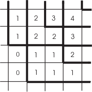
If we enumerate faces by the coordinates of their centers the height function can be regarded as $(N+1)\times(M+1)$ matrix with non-negative entries.

It is clear that there is a bijection between states of the $6$-vertex model with fixed boundary conditions and height functions with fixed boundary values.

Indeed, given a height function consider its “level curves”, i.e. paths on the grid $L_{N}$, where the height function changes its value by $1$, see Fig. 3. Clearly, this defines a state for the $6$-vertex model on $L_{N}$ with boundary conditions determined by the boundary values of the height function.

On the other hand, given a state in the $6$-vertex model, consider the corresponding configuration of paths. It is clear that there is a unique height function whose level curves are these paths and which satisfies the condition $h=0$ at the southwest corner.

It is clear that this correspondence is a bijection.

There is a natural partial order on the set of height functions with given boundary values. One function is bigger then the other if it is entirely above the other. There exist the minimum $h_{\rm min}$ and the maximum $h_{\rm max}$ height functions such that $h_{\rm min}\leq h\leq h_{\rm max}$ for all height functions $h$.

Thus, we can consider the $6$-vertex model as a theory of fluctuating discrete surfaces constrained between $h_{\rm max}$ and $h_{\rm min}$. Each surface occurs with probability given by the Boltzmann weights of the $6$-vertex model.

In the inhomogeneous $6$-vertex model the Boltzmann weights depend on the edge. Thus, we have $6N^{2}$ parameters $a_{i}(m,n)$, $b_{i}(m,n)$, and $c_{i}(m,n)$.

Let us assume that the inhomogeneity is only in magnetic fields, i.e. weights $a$,$b$, and $c$ do not change from edge to edge, but the magnetic fields $H(e)$, $V(e)$ do.

Let $\{P\}$ be the collection of paths corresponding to a state in the $6$-vertex model and $\{h(f)\}$ be the corresponding height function.

The proof is an elementary exercise.

Let $s(e)=\exp(H(e)$ for horizontal edges and $s(e)=\exp(V(e))$ for vertical edges. Then the probability of the state with the height function $h$ in such a model is

$$P_{q}(state)=\frac{\prod_{f}q_{f}^{h(f)}\prod_{\rm vertices}w_{0}(\rm vertex)}{Z}.$$

If $H(n,m)=H+am$ and $V(n,m)=V+bn$, the weights $q_{f}$ are the same for all faces $q_{f}=\exp(a+b)$ inside the lattice and the probability is given by

$$P(state)=\frac{q^{{\rm vol}(h)}\prod_{\rm vertices}w(\rm vertex)}{Z},$$

where $w(vertex)$ are the Boltzmann weights with constant magnetic fields and

$${\rm vol}(h)=\sum_{f\in L_{N}}h(f)$$

is the volume “under” the height function $h$.

If $q$ is fixed and is not equal to $1$ in the large volume limit, the system will be in a neighborhood of the minimal height function for $q<1$ and in the neighborhood of the maximal height function for $q>1$. One should expect that the partition function and local correlation functions will have finite limit.

When $q=\exp(\frac{\lambda}{N})$ for some $\lambda$, one should expect the existence of the limit shape. We will study this limit in Section 7.

It is clear from the definition of the height function that the slope should satisfy conditions $0\leq h,v\leq 1$.

The slope is simply the average number of horizontal and vertical edges occupied by paths per length.

The important corollary of the result of [Shef] is that, when a gradient Gibbs measure satisfies certain convexity conditions, there exists a unique translationally invariant measure. This implies that for the $6$-vertex model one should expect the uniqueness of such a measure for the generic slope.

Translationally invariant measures can be obtained by taking the thermodynamic limit of the 6-vertex model with magnetic fields on a torus. Then the slope is the Legendre conjugate to magnetic fields.

$$h=\lim_{N,M\to\infty}\langle\sigma_{e}\rangle=\lim_{N,M\to\infty}\langle\frac{N(hor)}{N}\rangle=\lim_{N,M\to\infty}\frac{1}{2NM}\frac{\partial\log Z}{\partial H}+\frac{1}{2}$$

for a horizontal $e$ and

$$v=\lim_{N.M\to\infty}\langle\sigma_{e}\rangle=\lim_{N,M\to\infty}\langle\frac{N(ver)}{N}\rangle=\lim_{N,M\to\infty}\frac{1}{2NM}\frac{\partial\log Z}{\partial V}+\frac{1}{2}$$

for a vertical $e$.

The weights $a$, $b$, and $c$ in this region satisfy one of the two inequalities, either $a>b+c$ or $b>a+c$.

If $a>b+c$, the Boltzmann weights $a$, $b$, and $c$ can be parameterized as

(4)

$$a=r\sinh(\lambda+\eta),b=r\sinh(\lambda),c=r\sinh(\eta)$$

with $\lambda,\eta>0$.

If $a+c<b$, the Boltzmann weights can be parameterized as

(5)

$$a=r\sinh(\lambda-\eta),b=r\sinh(\lambda),c=r\sinh(\eta)$$

with $0<\eta<\lambda$.

For both of these parametrization of weights $\Delta=\cosh(\eta)$.

The phase diagram of the model for $a>b+c$ (and, therefore, $a>b$) is shown on Fig. 5 and for $b>a+c$ (and, therefore, $a<b$) on Fig. 6.

When magnetic fields $(H,V)$ are in one of the regions $A_{i},B_{i}$ of the phase diagram, the system in the thermodynamic limit has the translationally invariant Gibbs measure supported on the corresponding frozen configuration. There are four frozen configurations $A_{1}$, $A_{2}$, $B_{1}$, and $B_{2}$, shown on Fig. 4. For a finite but large grid the probability of any other state is at most of order $\exp(-\alpha N)$ for some positive $\alpha$.

Local correlation functions are given by the value of the corresponding observable on the frozen state

$$\lim_{N\to\infty}\langle\sigma_{e_{1}}\dots\sigma_{e_{n}}\rangle_{N}=\sigma_{e_{1}}(S)\dots\sigma_{e_{n}}(S)$$

where $S$ is the one of the ferromagnetic states $A_{i},B_{i}$.

The frozen regions in the $(H,V)$-plane are described by the set of inequalities. The boundaries of these regions can be derived by analyzing the next to the largest eigenvalue of the row-to-row transfer matrix. The description is separated into two cases: $a>b+c$ and $b>a+c$. Notice that $a\neq b$ since $\Delta>1$.

$\bullet$ $a>b+c$, see Fig. 5,

	$\displaystyle\mbox{$A_{1}$-region:}\qquad V+H\geq 0,\qquad\cosh(2H)\leq\Delta,$
	$\displaystyle\qquad(e^{2H}-b/a)(e^{2V}-b/a)\geq(c/a)^{2},\qquad e^{2H}>b/a,\qquad\cosh(2H)>\Delta,$
	$\displaystyle\mbox{$A_{2}$-region:}\qquad V+H\leq 0,\qquad\cosh(2H)\leq\Delta,$
	$\displaystyle\qquad(e^{-2H}-b/a)(e^{-2V}-b/a)\geq(c/a)^{2},\qquad e^{-2H}>b/a,\qquad\cosh(2H)>\Delta,$
	$\displaystyle\mbox{$B_{1}$-region:}\qquad(e^{2H}-a/b)(e^{-2V}-a/b)\geq(c/b)^{2},\qquad e^{2H}>a/b,$
	$\displaystyle\mbox{$B_{2}$-region:}\qquad(e^{-2H}-a/b)(e^{2V}-a/b)\geq(c/b)^{2},\qquad e^{-2H}>a/b.$

$\bullet$ $b>a+c$, see Fig. 6,

	$\displaystyle\mbox{$A_{1}$-region:}\qquad(e^{2H}-b/a)(e^{2V}-b/a)\geq(c/a)^{2},\qquad e^{2H}>b/a;$
	$\displaystyle\mbox{$A_{2}$-region:}\qquad(e^{-2H}-b/a)(e^{-2V}-b/a)\geq(c/a)^{2},\qquad e^{-2H}>b/a;$
	$\displaystyle\mbox{$B_{1}$-region:}\qquad V-H\geq 0,\qquad\cosh(2H)\leq\Delta,$
	$\displaystyle\qquad(e^{2H}-a/b)(e^{-2V}-a/b)\geq(c/b)^{2},\qquad e^{2H}>a/b,\qquad\cosh(2H)>\Delta,$
	$\displaystyle\mbox{$B_{2}$-region:}\qquad V-H\leq 0,\qquad\cosh(2H)\leq\Delta,$
	$\displaystyle\qquad(e^{-2H}-a/b)(e^{2V}-a/b)\geq(c/b)^{2},\qquad e^{-2H}>a/b,\qquad\cosh(2H)>\Delta.$

The free energy is a linear function in $H$ and $V$ in the four frozen regions:

	$\displaystyle f=-\ln a-H-V\qquad\mbox{in}\quad A_{1},$
(6)		$\displaystyle f=-\ln b+H-V\qquad\mbox{in}\quad B_{2},$
	$\displaystyle f=-\ln a+H+V\qquad\mbox{in}\quad A_{2},$
	$\displaystyle f=-\ln b-H+V\qquad\mbox{in}\quad B_{1}.$

If $(H,V)$ is a region $D_{1}$ or $D_{2}$ the corresponding translationally invariant Gibbs measure has the slope $(h,v)$ given by (3). In this phase the system is disordered, which means that local correlation functions decay as a power of the distance $d(e_{i},e_{j})$ between $e_{i}$ and $e_{j}$ when $d(e_{i},e_{j})\to\infty$.

In the regions $D_{1}$ and $D_{2}$ the free energy is given by [SY]:

(7)		$\displaystyle f(H,V)$	$\displaystyle=$	$\displaystyle\min\Bigl\{\min_{\alpha}\Bigl\{E_{1}-H-(1-2\alpha)V-\frac{1}{2\pi i}\int_{C}\ln(\frac{b}{a}-\frac{c^{2}}{ab-a^{2}z})\rho(z)dz\Bigr\},$
				$\displaystyle\min_{\alpha}\Bigl\{E_{2}+H-(1-2\alpha)V-\frac{1}{2\pi i}\int_{C}\ln(\frac{a^{2}-c^{2}}{ab}+\frac{c^{2}}{ab-a^{2}z})\rho(z)dz\Bigr\}\Bigr\},$

where $\rho(z)$ can be found from the integral equation

(8)

$$\rho(z)=\frac{1}{z}+\frac{1}{2\pi i}\int_{C}\frac{\rho(w)}{z-z_{2}(w)}dw-\frac{1}{2\pi i}\int_{C}\frac{\rho(w)}{z-z_{1}(w)}dw,$$

in which

$$z_{1}(w)=\frac{1}{2\Delta-w},\qquad z_{2}(w)=-\frac{1}{w}+2\Delta.$$

$\rho(z)$ satisfies the following normalization condition:

$$\alpha=\frac{1}{2\pi i}\int_{C}\rho(z)dz.$$

The contour of integration $C$ (in the complex $z$-plane) is symmetric with respect to the conjugation $z\rightarrow\bar{z}$, is dependent on $H$ (see Appendix B) and is defined by the condition that the form $\rho(z)dz$ has purely imaginary values on the vectors tangent to $C$:

$${\rm Re}(\rho(z)dz)\Bigr|_{z\in\,\,C}=0.$$

The formula (7) for the free energy follows from the Bethe Ansatz diagonalization of the row-to-row transfer-matrix. Its derivation is outlined in Appendix B. It relies on a number of conjectures that are supported by numerical and analytical evidence and in physics are taken for granted. However, there is no rigorous proof.

There are two points where three phases coexist (two frozen and one disordered phase). These points are called tricritical. The angle $\theta$ between the boundaries of $D_{1}$ (or $D_{2}$) at a tricritical point is given by

$$\cos(\theta)=\frac{c^{2}}{c^{2}+2\min(a,b)^{2}(\Delta^{2}-1)}.$$

The existence of such points makes the $6$-vertex model (and its degeneration known as the $5$-vertex model [HWKK]) remarkably different from dimer models [KOS] where generic singularities in the phase diagram are cusps. Physically, the existence of singular points where two curves meet at the finite angle manifests the presence of interaction in the $6$-vertex model.

Notice that when $\Delta=1$ the phase diagram of the model has a cusp at the point $H=V=0$. This is the transitional point between the region $\Delta>1$ and the region $|\Delta|<1$ which is described below.

In this case, the Boltzmann weights have a convenient parameterization by trigonometric functions. When $1\geq\Delta\geq 1$

$$a=r\sin(\lambda-\gamma),b=r\sin(\lambda),c=r\sin(\gamma),$$

where $0\leq\gamma\leq\pi/2$, $\gamma\leq\lambda\leq\pi$, and $\Delta=\cos\gamma$.

When $0\geq\Delta\geq-1$

$$a=r\sin(\gamma-\lambda),b=r\sin(\lambda),c=r\sin(\gamma),$$

where $0\leq\gamma\leq\pi/2$, $\pi-\gamma\leq\lambda\leq\pi$, and $\Delta=-\cos\gamma$.

The phase diagram of the $6$-vertex model with $|\Delta|<1$ is shown on Fig. 7. The phases $A_{i},B_{i}$ are frozen and identical to the frozen phases for $\Delta>1$. The phase $D$ is disordered. For magnetic fields $(H,V)$ the Gibbs measure is translationally invariant with the slope $(h,v)=(\frac{\partial f(H,V)}{\partial H},\frac{\partial f(H,V)}{\partial V})$.

The frozen phases can be described by the following inequalities:

	$\displaystyle\mbox{$A_{1}$-region:}\qquad(e^{2H}-b/a)(e^{2V}-b/a)\geq(c/a)^{2},\qquad e^{2H}>b/a,$
	$\displaystyle\mbox{$A_{2}$-region:}\qquad(e^{-2H}-b/a)(e^{-2V}-b/a)\geq(c/a)^{2},\qquad e^{-2H}>b/a,$
(9)		$\displaystyle\mbox{$B_{1}$-region:}\qquad(e^{2H}-a/b)(e^{-2V}-a/b)\geq(c/b)^{2},\qquad e^{2H}>a/b,$
	$\displaystyle\mbox{$B_{2}$-region:}\qquad(e^{-2H}-a/b)(e^{2V}-a/b)\geq(c/b)^{2},\qquad e^{-2H}>a/b.$

The free energy function in the frozen regions is still given by the formulae (6). The first derivatives of the free energy are continuous at the boundary of frozen phases, The second derivative is continuous in the tangent direction at the boundary of frozen phases and is singular in the normal direction.

It is smooth in the disordered region where it is given by (7) which, as in case $\Delta>1$ involves a solution to the integral equation (8). The contour of integration in (8) is closed for zero magnetic fields and, therefore, the equation (8) can be solved explicitly by the Fourier transformation [Bax] .

The $6$-vertex Gibbs measure with zero magnetic fields converges in the thermodynamic limit to the superposition of translationally invariant Gibbs measures with the slope $(1/2,1/2)$. There are two such measures. They correspond to the double degeneracy of the largest eigenvalue of the row-to-row transfer-matrix [Bax].

There is a very interesting relationship between the $6$-vertex model in zero magnetic fields and the highest weight representation theory of the corresponding quantum affine algebra. The double degeneracy of the Gibbs measure with the slope $(1/2,1/2)$ corresponds to the fact that there are two integrable irreducible representations of $\widehat{sl_{1}}$ at level one. Correlation functions in this case can be computed using $q$-vertex operators [JM]. For latest developments see [BJMST].

References

- [AR] D. Allison and N. Reshetikhin, Numerical Study of the -Vertex Model with Domain Wall Boundary Conditions, Ann. Inst. Fourier (Grenoble) 55, 1847–1869, 2005.
- [AS] M. Abramowitz and I.A. Stegun, Handbook of Mathematical Functions with Formulas, Graphs, and Mathematical Tables, Dover Publications, 1972.
- [Bax] R.J. Baxter, Exactly Solved Models in Statistical Mechanics, Academic Press, San Diego, 1982.
- [BPZ] N.M. Bogoliubov, A.G. Pronko, and M.B. Zvonarev, Boundary Correlation Functions of the Six-Vertex Model, J. Phys. A 35, 5525–5541, 2002.
- [BIR] N.M. Bogoliubov, A.G. Izergin, and N.Y. Reshetikhin. Finite-size effects and infrared asymptotics of the correlation functions in two dimensions. J. Phys. A 20 (1987), no. 15, 5361–5369.
- [Bres] D.M. Bressoud, Proofs and Confirmations: The Story of the Alternating Sign Matrix Conjecture, Cambridge University Press, 1999.
- [BS] D.J. Bukman and J.D. Shore, The Conical Point in the Ferroelectric Six-Vertex Model, J. Stat. Phys. 78, 1277–1309, 1995.
- [CEP] H. Cohn, N. Elkis, and J. Propp, Local Statistics for Random Domino Tilings of the Aztec Diamond, Duke Math. J. 85, 117–166, 1996.
- [CKP] H. Cohn, R. Kenyon, and J. Propp, A variational principle for domino tilings. J. Amer. Math. Soc. 14, 297-346, 2001.
- [CP] F. Colomo, and A.G. Pronko,On two-point boundary correlations in the six-vertex model with domain wall boundary conditions. J. Stat. Mech. Theory Exp. 2005, no. 5, 05010, 21 pp.
- [DKS] R. Dobrushin, R. Kotecky, and S. Schlosman, Wulff Construction: a Global Shape from Local Interactions, AMS translation series, Providence RI, 104, 1992.
- [Elor] K. Eloranta, Diamond Ice, J. Statist. Phys. 96, 1091–1109, 1999.
- [FPS] P.L. Ferrari, M. Prähofer, and H. Spohn, Fluctuations of an Atomic Ledge Bordering a Crystalline Facet, cond-mat/0303162.
- [HWKK] H.Y. Huang, F.Y. Wu, H. Kunz, D. Kim, Interacting Dimers on the Honeycomb Lattice: an Exact Solution of the Five-Vertex Model, Physica A 228, 1–32, 1996.
- [Ize] A.G. Izergin, Partition Function of the -Vertex Model in a Finite Volume, (Russian) Dokl. Akad. Nauk USRR, 297, 331–333, 1987.
- [JM] M. Jimbo and T. Miwa, Algebraic Analysis of Solvable Lattice Models, CBMS Regional Conference Series in Math. 85, 1993.
- [BJMST] H. Boos, M. Jimbo, T. Miwa, F. Smirnov, Y. Takeyama, Hidden Grassmann structure in the XXZ model.hep-th/0606280
- [JS] C. Jayaprakash and W.F. Saam, Phys. Rev. B 30, 3916, 1984.
- [Ka] P. Kasteleyn, Graph Theory and Crystal Physics, Graph Theory and Theoretical Physics, 43, 1967.
- [KPZ] M. Kardar, G. Parisi, and Y.C. Zhang, Phys. Rev. Lett. 56, 889, 1986
- [K] R. Kenyon, Height fluctuations in the honeycomb dimer model, math-ph/0405052.
- [KO] R. Kenyon, and A. Okounkov, Planar dimers and Harnack curves. Duke Math. J. 131 (2006), no. 3, 499–524.
- [KOS] R. Kenyon, A. Okounkov, and S. Sheffield, Dimers and amoebae. Ann. of Math. (2) 163 (2006), no. 3, math-ph/0311005.
- [KW] R. Kenyon, and D. Wilson, Critical resonance in the non-intersecting lattice path model. Probab. Theory Related Fields 130 (2004), no. 3, 289–318.
- [KBI] V.E. Korepin, N.M. Bogolyubov, and A.G. Izergin, Quantum Inverse Scattering Method and Correlation Functions, Cambridge University Press, 1993.
- [Kor] V.E. Korepin, Calculation of Norms of Bethe Wave Functions, Commun. Math. Phys. 86, 391–418, 1982.
- [KZ] V. Korepin and P. Zinn-Justin, Thermodynamic Limit of the Six-Vertex Model with Domain Wall Boundary Conditions, J. Phys. A, 33, 7053–7066, 2000; Inhomogeneous Six-Vertex Model with Domain Wall Boundary Conditions and Bethe Ansatz, J. Math. Phys. 43, 3261–3267, 2002.
- [Kup] G. Kuperberg, Another Proof of the Alternating Sign Matrix Conjecture, Internat. Math. Res. Notices 3, 139–150, 1996.
- [Lieb] E.H. Lieb, Phys. Rev. 162, 162, 1967; E.H. Lieb, Phys. Rev. Lett. 18, 1046, 1967; 19, 108, 1967.
- [LW] E.H. Lieb and F.Y. Wu, Two Dimensional Ferroelectric Models, in Phase Transitions and Critical Phenomena, Vol. 1, ed. by C.Domb and M.S. Green, 321, Academic Press, London, 1972.
- [NK] J.D. Noh and D. Kim, Finite-Size Scaling and the Toroidal Partition Function of the Critical Asymmetric Six-Vertex Model, cond-mat/9511001.
- [Nold] I. M. Nolden, The Asymmetric Six-Vertex Model, J. Statist. Phys. 67, 155, 1992; Ph.D. thesis, University of Utrecht, 1990.
- [P] K. Palamarchuk, The -Vertex Model in Statistical Mechanics, Ph.D. thesis, Univesity of California at Berkeley, 2006.
- [PT] V.L. Pokrovsky and A.L. Talapov, Phys. Rev. Lett. 42, 65, 1979.
- [Shef] S. Sheffield, PhD Thesis, Stanford Univ. 2003.
- [Sm] F. Smirnov, Form factors in completely integrable models of quantum field theory, World Scientific, Singapore 1992.
- [SY] B. Sutherland, C.N. Yang, and C.P. Yang, Exact Solution of a Model of Two-Dimensional Ferroelectrics in an Arbitrary External Electric Field, Phys. Rev. Letters 19, 588–591, 1967.
- [SY1] B. Sutherland, Phys. Rev. Lett. 19, 103, 1967;
- [SZ] O.F. Syljuasen and M.B. Zvonarev, Directed-Loop Monte Carlo Simulations of Vertex Models, cond-mat/0401491.
- [Yang] C.P. Yang, Phys. Rev. Lett. 19, 586, 1967
- [Yang1] C.N. Yang and C.P. Yang, Phys. Rev. 150, 321, 1966; 150, 327, 1966
- [Z] P. Zinn-Justin, Six-Vertex Model with Domain Wall Boundary Conditions and One-Matrix Model, Phys. Rev. E 62, 3411-3418, 2000.
- [Z1] P. Zinn-Justin, The Influence of Boundary Conditions in the Six-Vertex Model, cond-mat/0205192.
- [Zub] J.-B. Zuber, On the Counting of Fully Packed Loop Configurations. Some New Conjectures, math-ph/0309057.
Appendix A The Partition Function of the Inhomogeneous -Vertex Model
Here we compute the partition function of the inhomogeneous -vertex model with the periodic boundary conditions applying the Bethe Ansatz method. We briefly describe the results and refer the reader to [KBI] for the details about the method.
Bethe Ansatz method works for the inhomogeneous 6-vertex model with the follwing inhomogeneities. One should parameters , ,.., to each row of the grid and parameters , ,.., to each column of the grid as shown on Fig. 14. Thus, a pair of spectral parameters is associated to the vertex of the grid. Boltzmann weights assigned to this point are:
where functions describe the parameterization of Boltzmann weights of the homogeneous model.
The partition function of the model with periodical boundary conditions can be written as
where is the row-to-row transfer matrix of the 6-vertex model [Bax]. The raw-to-raw transfer-matrix is the trace of the ”quantum monodromy matrix”:
Here is the product
which acts in . The matrix acts as the matrix
in the basis of the product of the 0-th and j-th factors in the tensor product. It acts trivially in other factors.
Let us denote the number of arrows pointing down in a row of the grid by . Denote by the corresponding subspace in the space of all possible states on the raw of length of vertical edges. The action of the transfer-matrix preserve these subspaces.
The Bethe Ansatz method gives the following result for the eigenvalues of :