LHC phenomenology of supersymmetric models beyond the MSSM

In this class of models one postulates very heavy right-handed neutrinos yielding the following superpotential below the GUT-scale:

For the neutrino mass matrix one obtains the well-known formula

Being complex symmetric, the light Majorana neutrino mass matrix in eq. (4) is diagonalized by a unitary $3\times 3$ matrix $U$ [23]

Inverting the seesaw equation eq. (4) allows to express $Y_{\nu}$ as [28]

where the $\hat{m}_{\nu}$ and $\hat{M}_{R}$ are diagonal matrices containing the corresponding eigenvalues. $R$ is in general a complex orthogonal matrix. We assume $R=1$ implying that $Y_{\nu}$ contains only “diagonal” products $\sqrt{M_{i}m_{i}}$.

In seesaw models of type II one adds a scalar $SU(2)$ triplet $T$ to generate neutrino masses. As this triplet carries also hypercharge one has to embed it in a $15$-plet of $SU(5)$ which has under $SU(3)\times SU_{L}(2)\times U(1)_{Y}$ the following decomposition [29]

In supersymmetric models one adds a pair $15$ and $\overline{15}$ to avoid anomalies below the GUT-scale. Below the GUT scale in the $SU(5)$-broken phase the superpotential reads

where the states with index 1 (2) belong the $15$-plet ($\overline{15}$-plet). The second term in eq. (8) is responsible for the generation of the neutrino masses yielding

Note that

i.e. $Y_{T}$ is diagonalized by the same matrix as $m_{\nu}$.

In addition there are the couplings $Y_{S}$ and $Y_{Z}$, which in principle are not determined by any low-energy data. In the calculation of lepton flavour violating observables both Yukawa couplings, $Y_{T}$ and $Y_{Z}$, contribute. Having a GUT model in mind we require for the numerical discussion later the $SU(5)$ boundary conditions $Y_{T}=Y_{S}=Y_{Z}$ at the GUT scale. As long as $M_{Z}\sim M_{S}\sim M_{T}\sim M_{15}$ gauge coupling unification will be maintained. The equality need not be exact for a successful unification. In our numerical studies we have taken into account the different running of these mass parameters but we decouple them all at the scale $M_{T}(M_{T})$ because the differences are small.

In the case of a seesaw model type III one needs new fermions $\Sigma$ at the high scale being in the adjoint representation of $SU(2)$. They have to be embedded in a $24$-plet to obtain a complete $SU(5)$ representation which decomposes under $SU(3)\times SU_{L}(2)\times U_{Y}(1)$ as

The fermionic components of $(1,1,0)$ and $(1,3,0)$ have exactly the same quantum numbers as $\nu^{c}$ and $\Sigma$. Thus, the $24_{M}$ always produces a combination of the type-I and type-III seesaw. In the $SU(5)$ broken phase the superpotential reads

As above we use at the GUT scale the boundary condition $Y_{N}=Y_{B}=Y_{X}$ and $M_{B}=M_{G}=M_{W}=M_{X}$. Integrating out the heavy fields yields the following formula for the neutrino masses at the low scale:

The boundary conditions at $M_{G}$ imply that at the seesaw scale(s) one still has $M_{B}\simeq M_{W}$ and $Y_{B}\simeq Y_{W}$ so that one can write in a good approximation

and one can use the corresponding decomposition for $Y_{W}$ as discussed in section 3.1.

The appearance of charged particles at scales between the electroweak scale and the GUT scale leads to changes in the beta functions of the gauge couplings [29, 30]. In the MSSM the corresponding values at 1-loop level are $(b_{1},b_{2},b_{3})=(33/5,1,-3)$. In case of one $15$-plet the additional contribution is $\Delta b_{i}=7/2$ whereas in case of $24$-plet it is $\Delta b_{i}=5$. This results in case of type II in a total shift of $\Delta b_{i}=7$ for the minimal model and in case of type III in $\Delta b_{i}=15$ assuming 3 generations of $24$-plets. This does not only change the evolution of the gauge couplings but also the evolution of the gaugino and scalar mass parameters with profound implications on the spectrum [30, 31]. Additional effects on the spectrum of the scalars can be present if some of the Yukawa couplings get large [31, 32, 33]. In figure 1 we exemplify this by showing the values of selected mass parameters at $Q=1$ TeV versus the seesaw scale for fixed high scale parameters $m_{0}=M_{1/2}=1$ TeV, $\tan\beta=10$ and $A_{0}=0$ where we have assumed that the additional Yukawa couplings are small. As expected, the effects in case of models of type II and III are larger the smaller the corresponding seesaw-scale is. The scalar mass parameters shown are of the first generation and, thus, the results are nearly independent of $\tan\beta$ and $A_{0}$.

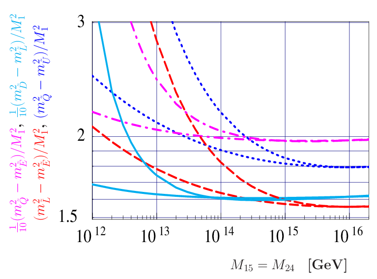
Note that in all three model types the ratio of the gaugino mass parameters is nearly the same as in the usual mSUGRA scenarios but the ratios and differences of the sfermion mass parameters change [30, 31]. One can form four ’invariants’ where at least at the 1-loop level the dependence on $M_{1/2}$ and $m_{0}$ is rather weak, e.g. $(m^{2}_{\tilde{L}}-m^{2}_{\tilde{E}})/M^{2}_{1}$, $(m^{2}_{\tilde{Q}}-m^{2}_{\tilde{E}})/M^{2}_{1}$, $(m^{2}_{\tilde{D}}-m^{2}_{\tilde{L}})/M^{2}_{1}$ and $(m^{2}_{\tilde{Q}}-m^{2}_{\tilde{U}})/M^{2}_{1}$. Here one could replace $M_{1}$ by any of the other two gaugino masses which simply would amount in an overall rescaling. In figure 3 we show these ’invariants’ in the leading-log approximation at 1-loop order to demonstrate the principal behaviour for seesaw type II with a pair of ${\bf 15}$-plets and seesaw type III with three ${\bf 24}$-plets. Due to the larger change in the beta-coefficient the effect is more pronounced in case of type III models. From this one concludes that in principle one has a handle to get information on the seesaw scale for given assumptions on the underlying neutrino mass model and assuming universal boundary conditions at the GUT scale. For the type-I, i.e. singlets only, of course $\Delta b_{i}=0$ and no change with respect to mSUGRA are expected. A detailed discussion can be found e.g. in [31].

Additional effects beside the ones on the spectrum discussed above can occur due to lepton flavour mixing entries in the sleptons mass matrix which are induced due to RGE effects by the additional Yukawa couplings. From a one-step integration of the RGEs one gets, assuming mSUGRA boundary conditions, a first rough estimate for the lepton flavour violating entries in the slepton mass parameters:

for $i\neq j$ in the basis where $Y_{E}$ is diagonal and $L_{ij}=\log(M_{G}/M_{i})\delta_{ij}$. The corresponding coefficient $a_{k}$ for seesaw type $k$ are: $a_{I}=1$, $a_{II}=6$ and $a_{III}=9/5$. All models have in common that the predict negligible flavour violation for the $R$-sleptons $m^{2}_{\tilde{E},ij}\simeq 0$. Sizable entries for the these parameters would be a clear hint for a left-right symmetric extension of the MSSM [35].

These flavour mixing entries induce on the one hand rare lepton decays, e.g. $\mu\to e\gamma$, and on the other hand lepton flavour violating decays of sleptons and neutralinos. As a typical example we show in fig. 3 the flavour violating decays of the heavier stau in a seesaw I scenario. One sees that branching ratios of at most a few per-cent can be reached close to the region excluded by $\mu\to e\gamma$ where $Y_{\nu}$ gets sizable. Also in case of seesaw type II one obtains similar results [31]. At the LHC however one will not be able to identify the individual branching ratios but one has to consider the complete cascade starting from the production and taking into account all steps of the various decays, e.g. $\tilde{q}_{L}\to q\tilde{\chi}^{0}_{2}\to ql_{i}^{\pm}{\tilde{l}}^{\mp}_{j}\to ql_{i}^{\pm}l_{k}^{\mp}\tilde{\chi}^{0}_{1}$. As typical examples we display in fig. 4 the obtainable cross section containing a $\mu^{\pm}\tau^{\mp}$ pair in the final state in case of seesaw models of type I and II for various values of $m_{0}$ as a function of $M_{1/2}$. Here the signal has been maximized by choosing the Yukawa couplings such that $BR(\mu\to e\gamma)=10^{-12}$ [36]. One sees that one gets at most signals up to $O(20-30)$ fb which clearly requires a large luminosity to be detected.

The superpotential of the bilinear $R_{p}\hskip-10.00002pt/\;\>$ model can be written as

In addition, one must include bilinear $R_{p}\hskip-10.00002pt/\;\>$ soft supersymmetry breaking terms

These terms induce mixings between the MSSM Higgs bosons and the left scalar neutrinos which in consequence also obtain vevs $v_{i}$ once electro-weak symmetry is broken. Usually one trades the $B_{i}$ by the $v_{i}$ using the corresponding tad-pole equations which are a consequence of eq. (18) as the connections to neutrino physics become more apparent.

The effective neutrino mass matrix at tree-level can then be cast into a very simple form

The “photino” mass parameter is defined as $m_{\gamma}=g^{2}M_{1}+g^{\prime 2}M_{2}$, $det(M_{\chi^{0}})$ is the determinant of the ($4,4$) neutralino mass matrix and $\Lambda_{i}\equiv\epsilon_{i}v_{d}+v_{i}\mu$ are the “alignment parameters”.

Due to the projective nature of eq. (19) the other two neutrino masses are generated only at 1-loop order. Generally the most important contributions come from loops with sbottoms and staus [44, 45]. However, there exist also parameter regions in the general $R_{p}\hskip-10.00002pt/\;\>$ MSSM where the sneutrino-anti-neutrino loop gives a sizeable contribution [46, 47, 48]. One finds that in order to explain the observed neutrino mixing angles one requires certain relations among the $R_{p}\hskip-10.00002pt/\;\>$ parameters to be satisfied [44], e.g. the maximal atmospheric angles requires $\Lambda_{\mu}\simeq\Lambda_{\tau}$.

Once R-parity is broken the LSP decays. The decays of a neutralino LSP have been studied in [51, 49]. Decay lengths for the neutralino are approximately fixed once the neutrino masses are fitted to experimental data. Typical lengths range from tens of cm for very light neutralinos to sub-millimeter for neutralinos of several hundred GeV [49]. One of the most exciting aspects of bilinear $R_{p}\hskip-10.00002pt/\;\>$, however, is the fact that once neutrino angles are fitted to the values required [13] by the neutrino oscillation data, the ratios of LSP decay branching ratios are fixed and correlate with the observed neutrino mixing angles, as illustrated for example in fig. 6. Measurements at the LHC should allow to test this prediction, if signals of SUSY are found [52].

Within $R_{p}\hskip-10.00002pt/\;\>$ SUSY any supersymmetric particle can be the LSP. It has been shown that within bilinear $R_{p}\hskip-10.00002pt/\;\>$ correlations between the measured neutrino angles and ratios of LSP decays can be found for all LSP candidates [53, 54, 55]. Thus, it is possible to exclude the minimal bilinear $R_{p}\hskip-10.00002pt/\;\>$ model experimentally at the LHC.

In spontaneous R-parity violation models [56, 37, 57] R-parity violation results from the minimization of the Higgs potential through nonzero sneutrino vacuum expectation values. If lepton number is ungauged this implies the existence of a Nambu-Goldstone boson - the majoron. However, a doublet majoron is ruled out by LEP measurements of the Z width [58]. Hence, viable spontaneous R-parity breaking models must be characterized by two types of sneutrino vevs, those of right and left sneutrinos, singlets and doublets under $\mathrm{SU(3)\otimes SU(2)_{L}\otimes U(1)_{Y}}$ respectively [59, 60]. These obey the “vev-seesaw” relation $v_{L}v_{R}\sim Y_{\nu}m_{W}^{2}$ where $Y_{\nu}$ is the small Yukawa coupling that governs the strength of R–parity violation [59, 60].

In this case the majoron is so weakly coupled that bounds from LEP and astrophysics [61] are easily satisfied. For example, the superpotential of [59] can be written as

The first three terms are the usual MSSM Yukawa terms. The terms coupling the lepton doublets to $\widehat{\nu}^{c}$ fix lepton number. The coupling of the field $\widehat{\Phi}$ with the Higgs doublets generates an effective $\mu$-term a lá the Next to Minimal Supersymmetric Standard Model (NMSSM) [62, 63, 64]. Note, that $v_{R}=\langle\tilde{\nu}^{c}\rangle\neq 0$ generates effective bilinear terms $\epsilon_{i}=Y_{\nu}^{i}v_{R}$ and that $v_{R}$, $v_{S}$ and $v_{L_{i}}$ violate lepton number and R-parity spontaneously. Neutrino oscillation data enforce $v_{L_{i}}^{2}\ll v_{R}^{2}$ and $v_{L_{i}}^{2}\ll v_{d}^{2}+v_{u}^{2}$ implying the majoron is mainly a singlet in this model [65, 66].

The existence of the majoron affects the phenomenology at colliders mainly in two ways: (i) the lightest Higgs can decay invisibly into two majorons [65, 66]. (ii) Also the decays of the lightest neutralino are affected, since the new decay channel $\chi^{0}_{1}\to J\nu$ is invisible at colliders. In ref. [67, 68] it has been shown that this mode can be close to 100% for certain parameter combinations implying that a large luminosity at the LHC might be required to detect R-parity violation. However, as can be seen in fig. 6 $chi^{0}_{1}\to J\nu$ is correlated with the decay $\mu\to Je$, thus allowing to probe for a complementary part of parameter space [50] with low energy experiments.

Spontaneous $R$-parity violation can also be obtained by enlarging the gauge group [69, 70, 71, 72, 73, 74, 75]. In this case the majoron would be the longitudinal component of an additional neutral heavy vector boson which can be produced in s-channel processes at the LHC.

In the following we mainly focus on mSUGRA models which are augmented by bilinear R-parity breaking parameters at the electroweak scale implying that one has eleven free parameters, namely $m_{0}$, $M_{1/2}$, $\tan\beta$, sign$(\mu)$, $A_{0}$, $\epsilon_{i}$, and $\Lambda_{i}$. In order to fit current neutrino oscillation data, the effective strength of R-parity violation must be small. This implies that supersymmetric particle spectra are expected to be the same as in the conventional R-parity conserving model, and that processes involving single production of SUSY states [76] are negligible at the LHC and that the only differences occur due to the decays of the LSP.

In these scenarios the lightest neutralino is the LSP and its main decay channels are $\tilde{\chi}^{0}_{1}\to\nu\ell^{+}\ell^{-}$ with $\ell=e$, $\mu$ denoted by $\ell\ell$; $\tilde{\chi}^{0}_{1}\to\nu\tau^{+}\tau^{-}$, called $\tau\tau$; $\tilde{\chi}^{0}_{1}\to\tau\nu\ell$, called $\tau\ell$. $\tilde{\chi}^{0}_{1}\to\nu q\bar{q}$ denoted $jj$; $\tilde{\chi}^{0}_{1}\to\tau q^{\prime}\bar{q}$, called $\tau jj$; $\tilde{\chi}^{0}_{1}\to\ell q^{\prime}\bar{q}$, called $\ell jj$; $\tilde{\chi}^{0}_{1}\to\nu b\bar{b}$, which we denote by $bb$; $\tilde{\chi}^{0}_{1}\to\nu b\bar{b}$, which we denote by $bb$; $\tilde{\chi}^{0}_{1}\to\nu\nu\nu$.

In ref. [77] a comparison has been performed between the reach of LHC for R-parity violating SUSY using the same cuts as for R-parity conserving models [78]. The main topologies are: Inclusive jets and missing transverse momentum; zero lepton, jets and missing transverse momentum; one lepton, jets and missing transverse momentum; opposite sign lepton pair, jets and missing transverse momentum; same sign lepton pair, jets and missing transverse momentum; tri-leptons, jets and missing transverse momentum; multi-leptons, jets and missing transverse momentum. Due to the reduced missing energy the all-inclusive channel will have a reduced reach in the parameter space. However, the decays of the neutralino increase the multiplicities of the multi-lepton channel. As an example we display in Fig. 7 the LHC reach in the three– and multi–lepton channels with/without R–parity conservation for an integrated luminosity of 100 fb^-1. These constitute the best standard channels for the discovery of bilinear R-parity violation.

The sizable decay length of the neutralino is quite useful as this topology has little, if any, background expected at the LHC. This feature has been exploited in ref. [77, 79], where a comparison has been performed between the reach of LHC for R-parity violating SUSY including explicitly the displaced vertex topologies. In figure 9 we present the displaced vertex reach in the $m_{0}$-$M_{1/2}$ plane for $\tan\beta=10$, $\mu>0$, $A_{0}=-100$ GeV. As one can see form this figure, the LHC will be able to look for the displaced vertex signal up to $m_{1/2}\sim$800 (1000) GeV for a large range of $m_{0}$ values and an integrated luminosity of 10 (100) fb^-1. Notice that the reach in this channel is rather independent of $m_{0}$. However, this signal disappears in the region where the stau is the LSP due to its rather short lifetime.

Next we discuss a tantalizing possibility, namely a double discovery at the LHC: (i) find evidence for supersymmetry, and (ii) uncover the Higgs boson. There are regions in parameter space where $\tilde{\chi}_{1}^{0}$ may have a sizeable branching ratio up to 22% into the channel $\nu h^{0}$ where $h^{0}$ is the lightest Higgs boson [80]. This would lead to displaced vertices containing two b-jets as a characteristic signature for Higgs production at the LHC [80]. The displaced vertex signal implies that also LHCb will have good sensitivity for such scenarios in particular in case of final states containing muons such as $\tilde{\chi}^{0}_{1}\to\nu\mu^{+}\mu^{-}$.Figure 9 demonstrates that the ATLAS and CMS experiments will be able to look for the signal up to $M_{1/2}\sim 700$ $(900)$ GeV for a LHC integrated luminosity of 10 (100) fb^-1. The hatched region in Fig. 9 indicates the LHCb reach for 10 fb^-1. Due to the strong cut on the pseudo–rapidity required by this experiment the reach for 2 fb^-1 is severely depleted and only a small region of the parameter space is covered.

Bilinear $R$-parity violation is essentially equivalent to tri-linear $R$-parity breaking with the superpotential

where the tri-linear couplings have the following structures

Obviously the phenomenology will be very similar if tri-linear $R$-parity violation is close to this structure. In the case of significant deviations from this structure is realized, one gets new interesting signatures. For example there exists light stau LSP scenarios where $\tilde{\tau}_{1}$ decays dominantly via 4-body decays such as $\tilde{\tau}_{1}\to\tau^{-}\mu^{-}u\bar{d}$ with long lifetimes leading to displaced vertices [81]. Another interesting signals are the resonant production of sleptons as discussed in [82, 83] or associated production of single sleptons with $t$-quarks [84].

An interesting question is to which extent one can measure deviations from the hierarchical structure above, e.g. the coupling $\lambda_{211}^{\prime}$ can still be of order $0.1$. It has been shown in [85] that in such a case one LHC will be able to measure such couplings of such a strength with an accuracy of about 10%.

References

- [1] Nilles H P 1984 Phys. Rept. 110 1–162
- [2] Haber H E and Kane G L 1985 Phys. Rept. 117 75–263
- [3] Witten E 1981 Nucl. Phys. B188 513
- [4] Dimopoulos S, Raby S and Wilczek F 1981 Phys. Rev. D24 1681–1683
- [5] Ibanez L E and Ross G G 1981 Phys. Lett. B105 439
- [6] Ellis J R, Hagelin J S, Nanopoulos D V, Olive K A and Srednicki M 1984 Nucl. Phys. B238 453–476
- [7] Steffen F D 2009 Eur. Phys. J. C59 557–588 (Preprint arXiv:0811.3347)
- [8] Weiglein G et al. (LHC/LC Study Group) 2006 Phys. Rept. 426 47–358 (Preprint hep-ph/0410364)
- [9] Nath P et al. 2010 Nucl. Phys. Proc. Suppl. 200-202 185–417 (Preprint arXiv:1001.2693) ”
- [10] Minkowski P 1977 Phys. Lett. B67 421
- [11] Hall L J and Suzuki M 1984 Nucl. Phys. B231 419
- [12] Kim J E and Nilles H P 1984 Phys. Lett. B138 150
- [13] Schwetz T, Tortola M A and Valle J W F 2008 New J. Phys. 10 113011 (Preprint arXiv:0808.2016)
- [14] de Gouvea A, Gopalakrishna S and Porod W 2006 JHEP 11 050 (Preprint hep-ph/0606296)
- [15] Gupta S K, Mukhopadhyaya B and Rai S K 2007 Phys. Rev. D75 075007 (Preprint hep-ph/0701063)
- [16] Choudhury D, Gupta S K and Mukhopadhyaya B 2008 Phys. Rev. D78 015023 (Preprint arXiv:0804.3560)
- [17] Weinberg S 1979 Phys. Rev. Lett. 43 1566–1570
- [18] Weinberg S 1980 Phys. Rev. D22 1694
- [19] Ma E 1998 Phys. Rev. Lett. 81 1171–1174 (Preprint hep-ph/9805219)
- [20] Yanagida T KEK lectures, 1979 Ed. O. Sawada and A. Sugamoto (KEK, 1979)
- [21] Gell-Mann M, Ramond P and Slansky R 1979 Print-80-0576 (CERN)
- [22] Mohapatra R N and Senjanovic G 1980 Phys. Rev. Lett. 44 912
- [23] Schechter J and Valle J W F 1980 Phys. Rev. D22 2227
- [24] Cheng T P and Li L F 1980 Phys. Rev. D22 2860
- [25] Foot R, Lew H, He X G and Joshi G C 1989 Z. Phys. C44 441
- [26] Borzumati F and Yamashita T 2009 (Preprint arXiv:0903.2793)
- [27] Kang S K, Morozumi T and Yokozaki N 2010 (Preprint arXiv:1005.1354)
- [28] Casas J A and Ibarra A 2001 Nucl. Phys. B618 171–204 (Preprint hep-ph/0103065)
- [29] Rossi A 2002 Phys. Rev. D66 075003 (Preprint hep-ph/0207006)
- [30] Buckley M R and Murayama H 2006 Phys. Rev. Lett. 97 231801 (Preprint hep-ph/0606088)
- [31] Hirsch M, Kaneko S and Porod W 2008 Phys. Rev. D78 093004 (Preprint arXiv:0806.3361)
- [32] Calibbi L, Frigerio M, Lavignac S and Romanino A 2009 JHEP 12 057 (Preprint arXiv:0910.0377)
- [33] Biggio C and Calibbi L 2010 (Preprint arXiv:1007.3750)
- [34] Hirsch M, Valle J W F, Porod W, Romao J C and Villanova del Moral A 2008 Phys. Rev. D78 013006 (Preprint arXiv:0804.4072)
- [35] Vicente A 2010 (Preprint arXiv:1010.0799)
- [36] Esteves J N et al. 2009 JHEP 05 003 (Preprint arXiv:0903.1408)
- [37] Ross G G and Valle J W F 1985 Phys. Lett. B151 375
- [38] Hirsch M and Valle J W F 2004 New J. Phys. 6 76 (Preprint hep-ph/0405015)
- [39] Dreiner H K 1997 (Preprint hep-ph/9707435)
- [40] Dreiner H K, Luhn C and Thormeier M 2006 Phys. Rev. D73 075007 (Preprint hep-ph/0512163)
- [41] Allanach B et al. (R parity Working Group) 1999 (Preprint hep-ph/9906224)
- [42] Barbier R et al. 2005 Phys. Rept. 420 1–202 (Preprint hep-ph/0406039)
- [43] Bartl A, Hirsch M, Vicente A, Liebler S and Porod W 2009 JHEP 05 120
- [44] Hirsch M, Diaz M A, Porod W, Romao J C and Valle J W F 2000 Phys. Rev. D62 113008 (Preprint hep-ph/0004115)
- [45] Diaz M A, Hirsch M, Porod W, Romao J C and Valle J W F 2003 Phys. Rev. D68 013009 (Preprint hep-ph/0302021)
- [46] Grossman Y and Haber H E 2001 Phys. Rev. D63 075011 (Preprint hep-ph/0005276)
- [47] Dedes A, Rimmer S and Rosiek J 2006 JHEP 08 005 (Preprint hep-ph/0603225)
- [48] Dedes A, Haber H E and Rosiek J 2007 JHEP 11 059 (Preprint arXiv:0707.3718)
- [49] Porod W et al. 2001 Phys. Rev. D63 115004
- [50] Hirsch M, Vicente A, Meyer J and Porod W 2009 Phys. Rev. D79 055023 (Preprint arXiv:0902.0525)
- [51] Mukhopadhyaya B, Roy S and Vissani F 1998 Phys. Lett. B443 191–195
- [52] De Campos F et al. 2010 (Preprint arXiv:1006.5075)
- [53] Hirsch M, Porod W, Romao J C and Valle J W F 2002 Phys. Rev. D66 095006 (Preprint hep-ph/0207334)
- [54] Restrepo D, Porod W and Valle J W F 2001 Phys. Rev. D64 055011
- [55] Hirsch M and Porod W 2003 Phys. Rev. D68 115007 (Preprint hep-ph/0307364)
- [56] Aulakh C S and Mohapatra R N 1982 Phys. Lett. B119 136
- [57] Santamaria A and Valle J W F 1989 Phys. Rev. D39 1780–1783
- [58] Amsler C et al. (Particle Data Group) 2008 Phys. Lett. B667 1
- [59] Masiero A and Valle J W F 1990 Phys. Lett. B251 273–278
- [60] Romao J C, Santos C A and Valle J W F 1992 Phys. Lett. B288 311–320
- [61] Raffelt G G Chicago, USA: Univ. Pr. (1996) 664 p
- [62] Barbieri R, Ferrara S and Savoy C A 1982 Phys. Lett. B119 343
- [63] Nilles H P, Srednicki M and Wyler D 1983 Phys. Lett. B120 346
- [64] Chamseddine A H, Arnowitt R L and Nath P 1982 Phys. Rev. Lett. 49 970
- [65] Hirsch M, Romao J C, Valle J W F and Villanova del Moral A 2004 Phys. Rev. D70 073012 (Preprint hep-ph/0407269)
- [66] Hirsch M et al. 2006 Phys. Rev. D73 055007 (Preprint hep-ph/0512257)
- [67] Hirsch M and Porod W 2006 Phys. Rev. D74 055003 (Preprint hep-ph/0606061)
- [68] Hirsch M, Vicente A and Porod W 2008 Phys. Rev. D77 075005 (Preprint arXiv:0802.2896)
- [69] Kuchimanchi R and Mohapatra R N 1993 Phys. Rev. D48 4352–4360 (Preprint hep-ph/9306290)
- [70] Huitu K and Maalampi J 1995 Phys. Lett. B344 217–224 (Preprint hep-ph/9410342)
- [71] Huitu K, Maalampi J and Puolamaki K 1999 Eur. Phys. J. C6 159–166
- [72] Fileviez Perez P and Spinner S 2009 Phys. Lett. B673 251–254 (Preprint arXiv:0811.3424)
- [73] Everett L L, Fileviez Perez P and Spinner S 2009 Phys. Rev. D80 055007 (Preprint arXiv:0906.4095)
- [74] Barger V, Fileviez Perez P and Spinner S 2009 Phys. Rev. Lett. 102 181802 (Preprint arXiv:0812.3661)
- [75] Ji X, Mohapatra R N, Nussinov S and Zhang Y 2008 Phys. Rev. D78 075032
- [76] Nogueira P, Romao J C and Valle J W F 1990 Phys. Lett. B251 142–149
- [77] de Campos F et al. 2008 JHEP 05 048 (Preprint arXiv:0712.2156)
- [78] Baer H, Mizukoshi J K and Tata X 2000 Phys. Lett. B488 367–372 (Preprint hep-ph/0007073)
- [79] de Campos F, Eboli O J P, Magro M B and Restrepo D 2009 Phys. Rev. D79 055008 (Preprint arXiv:0809.0007)
- [80] de Campos F, Eboli O J P, Magro M B, Restrepo D and Valle J W F 2009 Phys. Rev. D80 015002 (Preprint arXiv:0809.1637)
- [81] Dreiner H K, Grab S and Trenkel M K 2009 Phys. Rev. D79 016002 (Preprint arXiv:0808.3079)
- [82] Dreiner H K, Richardson P and Seymour M H 2001 Phys. Rev. D63 055008 (Preprint hep-ph/0007228)
- [83] Moreau G, Perez E and Polesello G 2001 Nucl. Phys. B604 3–31 (Preprint hep-ph/0003012)
- [84] Bernhardt M A, Dreiner H K, Grab S and Richardson P 2008 Phys. Rev. D78 015016 (Preprint arXiv:0802.1482)
- [85] Choudhury D, Godbole R M and Polesello G 2002 JHEP 08 004 (Preprint hep-ph/0207248)