Very high order lattice perturbation theory for Wilson loops
Abstract:
We calculate perturbative Wilson loops of various sizes up to loop order at different lattice sizes for pure plaquette and tree-level improved Symanzik gauge theories using the technique of Numerical Stochastic Perturbation Theory. This allows us to investigate the behavior of the perturbative series at high orders. We observe differences in the behavior of perturbative coefficients as a function of the loop order. Up to we do not see evidence for the often assumed factorial growth of the coefficients. Based on the observed behavior we sum this series in a model with hypergeometric functions. Alternatively we estimate the series in boosted perturbation theory. Subtracting the estimated perturbative series for the average plaquette from the non-perturbative Monte Carlo result we estimate the gluon condensate.
June 14-19,2010
Villasimius, Sardinia Italy
BI-TP 2010/33, HU-EP-10/58, DESY 10-174, Edinburgh 2010/29, LU-ITP 2010/006, LTH 888
1 Introduction
Since the introduction of the non-perturbative gluon condensate by Shifman, Vainshtein and Zakharov [1] there have been many attempts to obtain reliable numerical results for this quantity. Soon it became clear that lattice gauge theory provides a promising tool to calculate it from Wilson loops of sizes . In [2, 3] the plaquette was used whereas larger Wilson loops have been investigated in [4, 5]. In all cases it turned out to be crucial to know the perturbative tail of the Wilson loops as precisely as possible. In the last decade the application of Numerical Stochastic Perturbation Theory (NSPT) [6] pushed the perturbative order of the plaquette up to order [7] and even [8].
Apart from the extraction of the gluon condensate there is a general interest in the behavior of perturbative series in QCD (for a recent investigation see [9]). It is generally believed that these series are asymptotic, and assumed that for large the leading growth of the coefficients is factorial. Using the technique of NSPT one reaches orders of the perturbative series where a possible set-in of this assumed behavior can be tested - at least for finite lattices. In a more recent paper [10] Narison and Zakharov discussed the difference between short and long perturbative series and its impact on the determination of the gluon condensate.
In order to test to what extent improvement influences the behavior of the series we used in addition to the standard Wilson plaquette gauge action the tree-level improved Symanzik gauge action obtained by Weisz implementing Symanzik’s improvement programme [11].
We present perturbative calculations in NSPT up to order for Wilson loops using the Wilson action for lattice sizes with . In case of the Symanzik action we have computed the for . The computation for were performed on a NEC SX-9 computer of RCNP at Osaka University, for at the HLRN Berlin/Hannover, all others on Linux/HP - clusters at Leipzig University.
2 NSPT calculation up to
NSPT allows perturbative calculations on a finite lattice up to loop order which practically cannot be reached by the standard diagrammatic approach. A limit is set only by storage limitations and machine precision. The algorithm is introduced and discussed in detail in [6, 12] – we will not present it in this paper. For a detailed discussion of our results we refer to a forthcoming paper [13].
In order to fix the notation we write the general expansion of a Wilson loop of size in terms of the bare lattice coupling as
| (1) |
The coefficients are determined with NSPT and need to be known to a very good precision. In Figure 1 we show some results for these coefficients using the Wilson and Symanzik actions. One can see from that Figure that the statistical errors within the NSPT algorithm are rather small.
 |
 |
At all all the loops behave rather similarly, with the coefficents decreasing smoothly, in a similar way for all loop sizes. At smaller we see that the coefficients change sign and magnitude in a rather unpredictable way, particularly for large loops. We recognize some remarkable differences in the behavior between the two actions. First, for the Symanzik action the sign change in the expansion coefficients sets in at smaller Wilson loop sizes and is extended to larger loop orders . Second, the values of the Symanzik coefficients themselves are much smaller than their Wilson action counterparts. However, concerning the relative convergence behavior of the perturbative series (1) one should have in mind that the coupling used in computing physical observables is larger in the Symanzik case than in the Wilson case. At larger a seemingly asymptotic behavior (without sign changes) emerges.
One essential test for the validity of our perturbative calculations with NSPT is the signal/noise ratio. The expansion of the (integer) loop-order is constructed from even powers . Likewise one can build non-loop contributions which are half-integer and combined from odd powers of - they should vanish. In Fig. 2 we show that the loop contributions are always clearly separated in magnitude from the non-loop (noise) terms.
 |
 |
In addition we have to raise the question about the infinite volume limit of the loop series. This is related to the definition of the gluon condensate which is clearly a quantity. We follow the approach to extrapolate each coefficient at finite from to using the ansatz
| (2) |
3 Perturbative series at large order
It is generally assumed that perturbative series in continuum QCD are asymptotic. The situation might be different for perturbative series on finite lattices. Here we have both ultraviolet and infrared cut-offs and the series could be summed up to a finite value. With our computed coefficients up to order we are able to check this conjecture to a so far unrivaled level.
To perform such a summation we propose a model which is a generalization of the ansatz used in [14]. Denoting the generic coefficients of the perturbative series as we have found that a large set of our data above some loop order can be described rather well by the following ansatz for the ratio of subsequent coefficients
| (3) |
where are free parameters to be fitted. The series based on (3) can be summed up to for . For we obtain as solution
| (4) | |||||
As final hypergeometric model at we use
| (5) |
where is the coefficient of in the corresponding -expansion of . For other values of the formulae (4) and (5) change accordingly. In Fig. 3 we show two example plots for the ratio together with the model fit based on (3). In all investigated cases we do not observe a factorial growth of the coefficients up to order .
 |
 |
Formally, one can use model (5) (used for finite lattices) also for the extrapolated coefficients.
A possible alternative method consists in applying boosted perturbation theory, i.e. a rearrangement of the series in terms of a boosted coupling [8] (). Using the summed perturbative series we get the boosted summed plaquette as follows
| (6) |
In Fig. 4 we compare the summed perturbative series with as function of maximal loop order for . One clearly recognizes a distinct plateau reached by boosting for . The naive series is far from the model value computed from (5). Although this behavior of the boosted perturbation theory is found for finite , we assume that it remains valid also in the infinite volume limit.
 |
 |
4 Non-perturbative gluon condensate
Having under control the large order perturbative series we estimate now the non-perturbative gluon condensate . Being a physical quantity we should use the extrapolated values of the perturbative coefficients. On the other hand it could be useful to get numbers for the ”gluon condensate” at finite also: they provide some numerical insight how the infinite volume limit is approached.
We use the relation between the plaquette measured in Monte Carlo simulations and its perturbative analogue :
| (7) |
which defines the gluon condensate. In (7) denotes the standard -function with being its leading coefficient. From (7) it is obvious that the precision of the difference determines the reliability of an estimate for .
It has been proposed [10] to extract the gluon condensate taking into account a perturbative series of the plaquette summed to an order () from the following ansatz
| (8) |
where contains possible and contributions
| (9) |
The authors in [10] argued that non-zero values of the coefficient are an artefact due to a truncation of the series: above some value of this coefficient should vanish. Our perturbative series for both, the naive series (finite ) and boosted series () confirm their hypothesis: for boosted perturbation theory the -term decreases rapidly to zero for (see left of Fig. 5); for naive perturbation theory and finite one has to sum the series to much larger .
 |
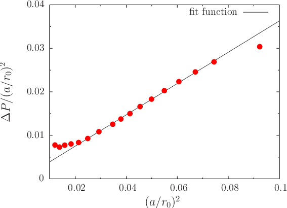 |
From the results obtained so far we conclude that the most reliable estimate for the gluon condensate can be obtained for the Wilson action using boosted perturbation theory. In the right of Figure 5 we show as function of using boosted perturbation theory with and our own non-perturbative plaquette measurements at different values and lattice sizes for . We clearly recognize a dominant linear behavior. The necessary conversion is accomplished for the plaquette action by the Necco-Sommer relation [15].
In Table 1 we give numbers for the quantity for finite and boosted perturbation theory at . For the perturbative values at finite we use the hypergeometric model as given in (5). The table shows that the boosted result for extrapolation agrees within errors with the model value at finite lattice size . The given errors have been estimated by varying the fit window .
| [GeV4] | fit range | ||
|---|---|---|---|
| 6 | |||
| 8 | |||
| 12 | |||
| , boosted |
Acknowledgements
This investigation has been supported partly by DFG under contract SCHI 422/8-1. We thank the RCNP at Osaka university and the HLRN Berlin/Hannover for providing computer resources.
References
- [1] M. A. Shifman, A. I. Vainshtein and V. I. Zakharov, Nucl. Phys. B 147 (1979) 385.
- [2] T. Banks, R. Horsley, H. R. Rubinstein and U. Wolff, Nucl. Phys. B 190 (1981) 692.
- [3] A. Di Giacomo and G. C. Rossi, Phys. Lett B 100 (1981) 481.
- [4] J. Kripfganz, Phys. Lett. B 101 (1981) 169; R. Kirschner, J. Kripfganz, J. Ranft and A. Schiller, Nucl. Phys. B 210 (1982) 567.
- [5] E.-M. Ilgenfritz and M. Müller-Preussker, Phys. Lett. B 119 (1982) 395.
- [6] R. Alfieri, F. Di Renzo, E. Onofri and L. Scorzato, Nucl. Phys. B 578 (2000) 383 [arXiv:hep-lat/0002018].
- [7] F. Di Renzo and L. Scorzato, JHEP 0110 (2001) 038 [arXiv:hep-lat/0011067].
- [8] P. E. L. Rakow, PoS LAT2005 (2006) 284 [arXiv:hep-lat/0510046].
- [9] Y. Meurice, Phys. Rev. D 74 (2006) 096005 [arXiv:hep-lat/0609005].
- [10] S. Narison and V. I. Zakharov, Phys. Lett. B 679 (2009) 355 [arXiv:0906.4312[hep-ph]].
- [11] P. Weisz, Nucl. Phys. B 212 (1983) 1.
- [12] F. Di Renzo and L. Scorzato, JHEP 0410, 073 (2004) [arXiv:hep-lat/0410010].
- [13] R. Horsley et al., in preparation.
- [14] R. Horsley, P. E. L. Rakow and G. Schierholz, Nucl. Phys. Proc. Suppl. 106 (2002) 870 [arXiv:hep-lat/0110210].
- [15] S. Necco and R. Sommer, Nucl. Phys. B 622 (2002) 328 [arXiv:hep-lat/0108008].