hep-th/1010.4396
FIT HE - 10-02
KYUSHU-HET 126
Accelerated Quark and
Holography for Confining Gauge theory
Kazuo Ghorokua11
1
gouroku@dontaku.fit.ac.jp,
Masafumi Ishiharab22
2
masafumi.ishihara@gmail.com,
Kouki Kuboc33
3
kkubo@higgs.phys.kyushu-u.ac.jp, Tomoki Taminatoc44
4
taminato@higgs.phys.kyushu-u.ac.jp
aFukuoka Institute of Technology, Wajiro, Higashi-ku
Fukuoka 811-0295, Japan
bDepartment of Electrophysics, National Chiao-Tung University, Hsinchu, Taiwan, R.O.C.
cDepartment of Physics, Kyushu University, Hakozaki, Higashi-ku
Fukuoka 812-8581, Japan
We show a constantly accelerated quark as a string solution of the Nambu-Goto action, which is embedded in the bulk background dual to the supersymmetric confining Yang-Mills theory. The induced metric of the world sheet for this string solution has an event horizon specified by the fifth coordinate. By an extended Rindler transformation proposed by Xiao, we move to the comoving frame of the accelerated quark-string. Then we find that this horizon is transferred to the event horizon of the bulk and the causal part of the accelerated quark is transformed to a static free-quark in the Rindler coordinate. As a result, the confinement of the Minkowski vacuum is lost in the Rindler vacuum. This point is assured also by studying the potential between the quark and anti-quark. However, the remnants of the original confining force are seen in various thermal quantities. We also discuss the consistency of our results and the claim that the Green’s functions will not be changed by the Rindler transformation.
1 Introduction
The observer, who is accelerated with a constant acceleration, , in the Minkowski space-time would observe thermal bath of particles with the temperature (the Rindler temperature) [1]-[3]. This phenomenon is known as the Unruh effect (see the review for example [4]). Recently, similar situation has been studied for the supersymmetric Yang-Mills theory in the context of the holography [5, 6, 7, 8]. In the approach of [6, 7], an accelerated quark has been introduced as string solutions of the Nambu-Goto action which is embedded in the background dual to the supersymmetric Yang-Mills theory. The solution in this background has been found by Xiao [6], and one finds an event horizon in the induced metric (in its world sheet) of this string configuration. The position of this horizon is specified by the fifth coordinate of the bulk.
Xiao has proposed an extended form of Rindler transformation (ERT) to move to a comoving frame of the accelerated quark. Performing this ERT, the event horizon appears in the bulk. Thus the theory dual to the ERT transformed geometry is considered as a finite temperature Yang-Mills theory. The temperature is given by the Rindler temperature . At the same time, the position of the bulk horizon can be put at the same fifth-coordinate point with the one of the world sheet horizon of the accelerated string. As a result, in the new coordinate, one finds a static string which connects the boundary and the event horizon of the bulk.
This is nothing but the free quark string-configuration in the Rindler vacuum. Since the theory dual to the is in the deconfinement phase, there is also a free quark in the Minkowski vacuum at zero temperature. However we should notice that the free quark in the one vacuum is not the same with the one in the other vacuum, because the static free-quark in the Minkowski vacuum cannot be transformed to the one of the Rindler vacuum by ERT, and vice versa. Anyway, in both theories dual to and to the one transformed by ERT, the quarks are not confined and chiral symmetry is not broken. So the confinement-deconfinement transition or chiral symmetry restoration has not been discussed as the thermal effect in the Rindler vacuum. Thus, it is remained as an important point to perform this analysis for the gauge theory in the confinement phase and also for the theory with the chiral symmetry broken in the Minkowski vacuum. Up to now, there is no such attempt.
Here we consider a confining Yang-Mills theory in the Minkowski vacuum in order to examine the property of its Rindler vacuum, which is obtained by performing the ERT. As a concrete model, we consider a supersymmetric background solution of type IIB theory. This background is dual to supersymmetric Yang-Mills theory, and the quark is confined in this theory[9]-[11]. In other words, it is impossible to find a free quark string solution for the Nambu-Goto action embedded in this background.
Then we firstly solve the equation of motion for the Nambu-Goto action to find a constantly accelerated quark-string solution, which has a similar functional form to the Xiao’s one. Actually, we could find such a solution. Then the original coordinate with the Minkowski vacuum is transformed to the comoving coordinate of the accelerated string solution by the ERT given by Xiao. After performing this transformation, we could find the free-quark string configuration in the Rindler vacuum as in the case of . This implies that this Rindler vacuum is in the quark deconfinement phase. However, we should again notice that the quark in the Rindler vacuum is not the one in the Minkowski vacuum. Then this phase change between the Minkowski and Rindler vacuum cannot be interpreted as the phase transition, which is seen in the usual finite temperature theory. In the latter case, the quark is considered to be common in both phases.
In the new coordinate vacuum, the dual theory can be regarded as the thermal Yang-Mills theory with the Rindler temperature. Its thermal properties are then examined furthermore, and we could assure that the confinement has been lost at any value of the finite Rindler temperature. So, there is no critical temperature in this case. On the other hand, some remnants of the confining force are seen in various quantities. The situation is similar to the case of the finite temperature theory dual to the -Schwartzschild background.
One may consider that our result seems to be inconsistent with the statement of [2]. There is a claim that the quark deconfinement is not expected in the Rindler vacuum. This is based on the equivalence of the vacuum expectation value of Green’s functions. However, it can be understood that our calculations and the results derived from them are not contradicting with the claim given in [2] based on the Green’s functions since our results are derived from the Wilson-loop calculation in each vacuum for the corresponding quarks, which cannot be related by the coordinate transformation as mentioned above. This point is explained more in the section 5.
In section 2, we give the setting of our model for the supersymmetric confining Yang-Mills theory. In section 3, the accelerated string solutions for the supersymmetric theory are given, and then the effect of the confining force is examined by comparing with the solution given for background. In section 4, new coordinate is given by the ERT, and we find the same Rindler temperature with the one given for . The thermal effects are studied to see that the confinement is lost in the Rindler vacuum. However, the remnant of the confining force has been observed in the Wilson-loop calculation and the drag force. In section 5, a brief comment related to the work of 4D field theory is given. The summary and discussions are given in the final section.
2 D3 model for confining Yang-Mills theory
We consider 10D IIB model retaining the dilaton , axion and self-dual five form field strength . Under the Freund-Rubin ansatz for , [9, 10], and for the 10D metric as or , we find the solution. The five dimensional part of the solution is obtained by solving the following reduced 5d action,
| (1) |
which is written in the string frame and taking .
The solution is obtained under the ansatz,
| (2) |
which is necessary to obtain supersymmetric solutions. And the solution is expressed as
| (3) |
Then, the supersymmetric solution is obtained as
| (4) |
where and . And represents the vacuum expectation value (VEV) of gauge fields condensate [10, 11]. In this configuration, the four dimensional boundary represents the =2 SYM theory. In this model, we find quark confinement in the sense that we find a linear rising potential between quark and anti-quark with the tension [9, 11]. However, chiral symmetry is preserved in the sense that the vacuum expectation value of the order parameter is zero. In other words, the dynamical mass generation of massless quarks does not occur.
3 Accelerating string solution
Here we restrict to the supersymmetric case. The metric for the supersymmetric case (4) is given as,
| (5) |
where . The world sheet coordinates of the string are taken as , and it is assumed to be stretching in the direction . Then the induced metric on the world sheet of the string is given as
| (6) | |||||
| (7) | |||||
| (8) |
Then the Nambu-Goto action for a string stretching in the direction is given as follows,
| (9) |
for the world sheet of the string , where , , and
| (10) |
The equation of motion for is obtained as
| (11) |
| (12) |
where dash and dot denotes the derivative with respective to and respectively as given above.
case
Before solving (11), we briefly review Xiao’s analytic solution given for or , namely in background. In this case, the solution is obtained as
| (13) |
This solution represents the accelerated quark in the supersymmetric Yang-Mills theory in the deconfinement phase. The value denotes the acceleration of the quark sitting at the boundary. The speed of the string to -direction depends on the position , and it exceeds light velocity in the region .
We notice here the following point. For this solution, the induced metric of the string world sheet is given as
| (14) |
This implies that has a zero point at and this point could be regarded as the horizon on the world sheet. So we could see the Hawking radiation of fields on the world sheet. However, there is no horizon in the 5D bulk background, so this situation is interpreted as the gauge field radiation of the accelerated color charged particle, namely the quark.
In the present case, the world sheet metric of the accelerated string are time-dependent and non-diagonal, then we should go to the other coordinate which would provide a clear vacuum of the theory. This is performed by the Rindler coordinate transformation given by (24)-(26) in the next section. In this case, we find the following world sheet metric
| (15) | |||||
| (16) | |||||
| (17) |
These represent the bulk metric at the same time, so we find the horizon of the world sheet and the one of the bulk are common. As a result, we find the thermal bath of the radiation in the new coordinate. This is known as Unruh effect.
Here we give some comment on the string. In the new coordinate, the string world sheet is transformed to , and it stretches in the direction . Then the string solution given above is transformed as
| (18) |
The new horizon point is equivalent to the point of , which is the horizon point of (14). The string represented by (18) is the straight line from the horizon to the boundary . Then the part of the string in Minkowski coordinate has been hidden in the thermal bath (inside the horizon) in the new vacuum. We can see the similar situation for the accelerated solutions given in different form of background.
case
In the next, we solve the above equation (11) for the case of non-trivial dilaton, namely for . Also in this case, we solve (11) by assuming the following functional form,
| (19) |
We would find at large where the effect of could be neglected. But the function deviates from when decreases, then it may be written as
| (20) |
where is expected to be proportional to . These points are seen as follows.
The equation (11) is rewritten as the one of as follows,
| (21) |
where prime denotes the derivative with respect to . We consider firstly the asymptotic behavior near the boundary (). Substituting into this equation (21), we find
| (22) |
at large . Here is an arbitrary constant as in . The solution has two arbitrary constants since the equation is the second order differential equation. Then we can set the asymptotic value of as for any as the boundary condition used here. However this condition restricts the boundary condition in the infrared region of small .
For the boundary condition, , the solution with positive deviates definitely from at small . In general the zero point of increases with , namely
| (23) |
This is obtained when we fix the point at as for any . On the other hand, the value of moves to the large value with increasing when we fix . The situation depends on the boundary condition in solving the equation of motion of . The understandable situation would be to fix the acceleration of the quark as by . In this case, the “horizon” on the string moves to larger value and the string configuration is modified from with increasing . However the Rindler temperature, which is obtained after a coordinate transformation where the string is seen to be static, does not depends on and also other parameter coming from the coordinate transformation. On the other hand, Rindler Temperature changes with the parameter of ERT, namely . We show this point in the next section.
For , we give here the numerical solutions. The solutions for are shown in the Fig. 1 and it is compared with the one of . We can see the zero point of moves to the larger value of as stated above.

4 Extended Rindler Transformation
Then we move to the comoving coordinate of the accelerated quark. Usually this is performed by the transformation among the two coordinate in the 4D space-time, time and the one of the accelerated direction, as seen in [2, 5]. However here we use another form of Rindler transformation proposed by Xiao [6]. This transformation is performed among the three coordinates, time, the accelerated direction and the fifth coordinates of the original AdS5 space-time, namely for . We call this as the extended Rindler transformation (ERT). After the transformation, in the new coordinate, the accelerated quarks given above in the original coordinate are seen as static and they are in a thermal bath with a finite temperature. Especially, we notice that these quarks are moving as free particles. In this sense, the quark is not confined in the dual gauge theory for the Rindler coordinate given by the extended Rindler transformation. We study the details of this point in the followings.
For the case of , the comoving coordinate, , of this accelerated quark is obtained from the original coordinates, , by the following extended coordinate transformation [6],
| (24) | |||||
| (25) | |||||
| (26) |
Then, the new metric is given as
| (27) |
and the above string configuration (13) is given by
| (28) |
which is static since it is independent of the new time coordinate . This string represents a free** * Here, “free” means that the quark is not bounded with an anti-quark as a meson. quark string which connects a D-brane put at some and the event horizon .
We should notice here that we can replace the parameter by other value, for example by , in the above coordinate transformation (24)-(26). In this case, we find the transformed accelerated string at
| (29) |
where we imposed the condition that the position of the quark on the boundary is transformed to . In this new coordinate with , the Rindler temperature is obtained as . We however set here as for the simplicity. In this case, the Rindler temperature is directly related to the acceleration of the particles as in the particle physics.
For the case of , we consider the following similar transformation,
| (30) | |||||
| (31) | |||||
| (32) |
where denotes the acceleration of the quark at the boundary. Then we find the new coordinate,
| (33) | |||||
where prime represents the derivative with respect to , and we set as
| (34) |
to eliminate the . Then is related to by solving (34) as
| (35) |
where is an arbitrary constant. Then we find again the Rindler coordinate for and , except for the prefactor . In the present case, we change the radial coordinate from to , then we have
| (36) |
The accelerated strings therefore can be seen in the same Einstein frame coordinate also in the confining phase (for ).
Transformed String Configurations
We consider how the string configuration of the accelerated strings is seen in the comoving coordinate. The configuration is different from the case. The new configuration is shown in - plane by using the relation,
| (37) |
which is obtained from the form of the solution, . Then, using the solution, , we find the string configurations in the Rindler coordinate in terms of the equation (37).
The boundary condition should be taken as at fixed since in represents the acceleration of the quark at the boundary. This implies from (37). In the Fig. 2, some examples of the solution for with are shown.

When we set , we obtain , which is the straight line of , namely the -axis. The larger q becomes, the larger the deviation of the string configurations from the straight line grows. (i) However, in any case, each string configuration shows the free quark state in a heat bath of Rindler temperature and (ii) the horizon is given by the point, (or ), where the velocity of the string to -direction in the original coordinate arrives at the speed of the light.
Temperature and Asymmetry of three space
Here we consider the temperature from two viewpoints. Firstly, it could be given from the condition to evade a conical singularity in plane for the Euclidean metric ().
It is seen near the horizon. By setting as , the metric (36) is rewritten for small as follows
| (38) |
where
| (39) |
From the above, the temperature is given by
| (40) |
for fixed . Here we must notice that the prefactor depends on the new coordinate , then the temperature is well defined only for fixed in this definition. However, we notice that the temperature given by (40) is independent of , in other words, the thermal equilibrium with the temperature would be seen at any point of , then this temperature is well defined in the three dimensional space, .
The other way to define the temperature is given by considering the timelike Killing vector , which satisfies
| (41) |
In this case, the surface curvature at the horizon is given as
| (42) |
then we obtain the same result with (40),
| (43) |
So the temperature could be well defined in the Rindler coordinate, but the three space, , is asymmetric. It is separated to the longitudinal () and the transverse (-) directions. This asymmetric behavior is also reflected to the color force, and it can be seen through the dilaton which affects the force between the quark and the anti-quark as being found through the Wilson-Loop, its analyses are given in the next section.
Actually, the gauge coupling constant is defined by and it depends on and as follows,
| (44) |
This implies that the Yang-Mills force depends on the energy scale and also on the coordinate in the real three space. In the present case, the temperature is finite and the Yang-Mills force between a quark and anti-quark is completely screened when they are separated by the distance () larger than a critical value (). Namely the quark is independent of the anti-quark which is separated by the distance , but we know that the quark can feel the force from the anti-quark in the region of and this force is nearly equivalent to the one given at zero-temperature.
In the present case, we find the linear rising force in the region of , where defines the ultra-violet region of the conformal symmetric limit. And we find the tension parameter [11]
| (45) |
at zero temperature in the present model. Then we expect the tension parameter in the Rindler coordinate would be given by
| (46) |
which is however coordinate dependent. We can assure this point through the Wilson-Loop calculation given below. Therefore we study the dynamical properties in this vacuum by separating to two cases, the longitudinal and transverse directions in the three dimensional space in the new coordinate.
4.1 Wilson Loop and the Force Between Quarks
From the gauge coupling given above (44), we can say that the force between the quark and anti-quark would depend on and also on . In our original metric, the quarks are confined due to the strong infrared gauge coupling constant, namely it diverges for . In the new coordinate (Rindler coordinate), the infrared strong-force would be screened by the fluctuations of the thermal matter with the temperature . The situation would be parallel to the case of the AdS-Schwartzschild background which is dual to the high temperature gauge field theory. Due to this screening, we would find deconfinement phase in the Rindler vacuum. This is the Unruh effect in the confinement theory. In order to assure this point, we study the force between the quark and the anti-quark, which are represented by the static strings in the Rindler vacuum (36).
(a) Strings Stretched to the longitudinal () direction
Consider the string which is extending to the direction. Taking its world sheet as , then the Nambu-Goto action of this string is given as
| (47) |
where , namely the prime denotes the derivative with respect to . The equation of motion for is given as
| (48) |
We notice here that the dilaton depends on and , and we find
| (49) |
then the right hand side of (48) is not zero, so we cannot obtain the symmetric U shaped string configuration. We therefore solve the equation of motion by using a parameter along the string. †† † The parameter introduced here has nothing to do with the one given in (24)-(26) in the above.
Before studying the Wilson loop, we like to show that the Rindler coordinate is dual to the deconfinement phase of the gauge theory. We consider the energy of the string, which is given by changing the variable from to as
| (50) |
| (51) |
If quarks are confined, we would find
| (52) |
where denotes the tension of the linear rising potential between the quark and the anti-quark, which are separated by , and is the minimum point of . In the present case, and , so we cannot find linear potential with a definite tension for large . In other words, the quarks are not confined. The main reason of this deconfinement might be the screening of the color force at finite distance due to the thermal effect of the thermal bath with the Rindler temperature given above.
Reparametrization invariant formulation
These points can be seen more explicitly by calculating the Wilson loop in the Rindler vacuum. As mentioned above, we rewrite the action (47) by using the parameter along the string as follows
| (53) |
| (54) |
where the dot denotes the derivative with respect to . We notice that the above Lagrangian is reparametrization invariant with respect to , then we can give the Hamiltonian where
| (55) |
and we obtain
| (56) |
| (57) |
Notice that we can use the Hamiltonian instead of . This is allowed since the theory we are solving is written in the reparametrization invariant form. In this case, we impose the Hamiltonian constraint as in the gravitational theory,
| (58) |
Under this constraint, we find that the difference of the solutions of the Hamilton’s equations written by and is in the parametrization of the solution. For example we write the solution as or , where
| (59) |
So in both cases of and , we will find the same string configuration.
Then we can derive the equations of motion of the string by the following Hamilton’s equations of ,
| (60) |
| (61) |
Boundary Condition and Numerical Solutions


Solving the above equations (60) and (61) numerically, the solutions are obtained as the functions of . We solve them with the boundary conditions,
| (62) |
and is given from the constraint at as,
| (63) |
Here denotes the end point of the string, and it is fixed so that this point is interpreted as the flavor brane’s position or a UV cutoff nearby the boundary. And denotes the bottom of the string solution. This point is varied to obtain the string solutions with various different energy , which is obtained by substituting the solution into the following equation,
| (64) |
Here the values of and are obtained from the solution by solving the following equations,
| (65) |
They indicates the two end points of the string solution.
As for , it denotes the coordinate at the bottom of the string solution and it controls the end point values and . Then, we adjust such that and . In this case, the distance () between the quark and anti-quark for these solutions is given as
| (66) |
In our present calculation, is cut at and the quarks are supposed to be at this point. This regularization does not affect on the large behavior of the Wilson loop estimations.
We show the results in the Fig.3 for the region , where the parameters are set as , , (left) and (right).
For sufficiently large compared to the temperature , as mentioned above, we can see the color force with a definite tension before the screening effects becomes dominant. In this region, the string energy is approximated as in terms of the tension and the length of the string. In the present case the tension is given by (46), however is measured in the direction and the tension depends on . Therefore the energy could be estimated as follows,
| (67) |
Actually, we can see a good fit with this curve for low temperature case , and the numerical result as shown in the left figure of Fig.3.
On the other hand, at high temperature, for the case of , we can find that the potential is screened before it meets the dashed curve as shown in the right one of Fig.3. As for the screening, we can see it through the existence of the maximum point () of which we discussed in previous subsection. This point moves smaller with the increasing temperature as expected from the usual high temperature theories in the confinement phase.
The same analysis has been performed also for . In this case, the force becomes weak even if is small, so the screening becomes dominant at rather small and it becomes difficult to see the remnant of the confinement force. We abbreviated here to show the numerical results.
(b) Strings Stretched to the transverse direction
Next, we consider the string stretched to the transverse direction, for example to direction which is transverse to the accelerated direction . In this case, the action is given as
| (68) |
where . And . is also retained since we can’t fix as a constant value as can be seen from the equations of motion for .
In order to obtain the relation of and as given above, we must obtain the string solutions. It is convenient to solve the equations after rewriting the action in the reparametrization invariant form as above,
| (69) |
where dot denotes the derivative with respect to the parameter . Then we have the canonical momentum,
| (70) |
and the following Hamiltonian
| (71) |
Then we can solve the equations of motion by the following Hamilton equations,
| (72) |
| (73) |
| (74) |
Boundary Condition and Numerical Solutions
Solving the above equations numerically, we imposed the following boundary conditions,
| (75) | |||
| (76) |
and is given from the constraint at as
| (77) |
In this case, the distance between the quark and the anti-quark is measured in the direction of by setting the coordinate as the same value at the two end points. Namely, we suppose at ,
| (78) |
where and is defined as (65) and () denotes the position of the quark (anti-quark). Then the distance between quark and anti-quark is obtained as,
| (79) |
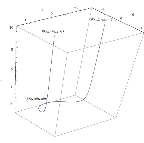
We must be careful about the following fact that, as shown above, the color force is in the present case depending on and . Now we like to see the force in the direction through the solution of (72)-(74). So we should solve these equations by imposing the condition that the end point coordinate is kept as a fixed value. So here we must tune the boundary values, and in order to realize the same for each solution. Here, we obtain the solution for
and a typical string solution in the present case is shown in Fig.4.
Defining the energy of the quark and anti-quark system as (64) in the case of (a),
we can see the relation of and as above. A typical results are shown in the Fig. 5. In this case we can see the linear rising part before the screening. This rising part is fitted by the formula
| (80) |
where would be approximately given by the on the horizon () as,
| (81) |


As for the upper part of - relation, the curve increases with decreasing . This point is understood as follows. The upper part is obtained by pulling the bottom point of the string to near the horizon. Then the lower part of the string grows to the direction of and the energy of the string becomes large as shown in Fig.4. This kind of behavior cannot be seen in the case of the AdS-Schwartzschild background.
Screening Length and Temperature
In the next, we turn to the temperature dependence of the screening length, which is defined by the maximum value of allowed for a given temperature. It is denoted by , and it usually decreases with temperature as observed in the theory dual to the AdS-Schwartzschild background [12]. We find finite for any finite or temperature as the reflection of the screening of the color force. Our result of the relation between and is given in the Fig.6.
The dotted (solid) curve represents the results from the Wilson loop stretched in the transverse () (longitudinal ()) direction. The behavior of two curves clearly differs from each other in the small region. This implies that the color force enhancement in the longitudinal direction at low temperature is greater than the force in the transverse direction. In the case of the transverse direction, the behavior is similar to the case of the AdS-Schwartzschild background, where is almost constant or varies slowly with the temperature. On the other hand, at high temperature, the screening becomes dominant and the asymmetric behavior disappears. As a result, the two curves coincident at large (at high temperature) region. This is also assured from the fact that the potentials in two cases approaches to the similar form.

4.2 Trailing string and drag force
Next we examine the drag force working on the quark moving with a constant velocity in the hot gluons. This is done by studying the trailing solution, which was discussed in [13, 14, 15] in the AdS-Schwartzschild background. In the present case, it is performed in the Rindler background (36) given here. According to the work [13, 14, 15], we consider a heavy quark moving with a fixed velocity in the thermal medium. This running quark is expressed through a string with the velocity , and its end point is on the boundary.
When we choose the coordinate as the moving direction, the string solution is supposed as
| (82) |
For the coordinate (36), however, it is easily found that there is no such a form of solution. The reason is that the dilaton depends on both time and as . Then the equation of motion for contains time explicitly through the dilaton as,
| (83) |
As a result, should depends on and also on to satisfy the equation of motion.
Therefore, the moving direction should be chosen as or in order to obtain a string solution with a constant velocity as given in the r.h.s. of (82) and to see the conserved momentum flow along the string from the boundary to the horizon. So we embed the string with its world sheet () into the space through the ansatz that constant and
| (84) |
We notice that we should keep dependence of also in this case due to the non-trivial dilaton. Then, the induced metric of the string is given as
| (85) | |||||
| (86) | |||||
| (87) |
and the Nambu-Goto action of this string is written as
| (88) | |||||
From this action, we find equation of motion for , and its conserved conjugate momentum () is obtained as
| (89) |
Here we notice that we also find . However there is no momentum in the direction now, so we don’t need to consider the drag force in this direction. However, we must solve both and in order to obtain as seen from Eq. (89). As a result, the string configuration moving with a constant velocity is deformed also to direction. The profile of such string is shown in the Fig. 7.

Here we give the following comment instead of showing the numerical behavior of the drag force. The drag force on the quark can be determined by the momentum flow which is lost as the flow from the string to the horizon [15]. We find the horizon on the string world sheet at from (85),
| (90) |
which depends on and . And , namely, it is larger than the bulk horizon. Another point to be noticed is that the velocity is constrained in the present case as
| (91) |
for fixed .
In any case, thus, we can estimate the drag force at the horizon , where and dependence disappears, as
| (92) |
Here we notice the following two points. First, we can see , then the force observed at the horizon is only the drag force for dragging the string to the direction. While the value of is determined by solving for the first time, it is not performed here. In the second, the force is modified by the color force due to the dilaton from the form which is proportional to the temperature, .
Finally as for the friction constant , one can define it as
| (93) |
where denotes the quark mass, and is written as,
| (94) |
For small , we find and , then we get
| (95) |
Then the friction constant is related to the radiation power given in background [6].
In the case of the -Schwarzschild background, the friction constant is given as follows [14],
| (96) |
On the other hand, in the limit of , (95) leads to
| (97) |
since in this limit. Thus we recognize the difference of factor four between (97) and (96). This point should be explained from some physical insight, but it is remained as an open problem here.
5 Relation to the 4D Field Theory
Here we give a comment on the statement for the Unruh effect given in [2], where the analysis is performed within the 4D field theory. The main result is that the vacuum expectation values (VEV) of any Green’s functions in the vacuum of Minkowski space-time are the same with the one of the Rindler space-time when the calculation is restricted to the same Rindler wedge in the Minkowski coordinate. So one may consider that the phase of the Minkowski vacuum cannot be changed in the Rindler vacuum since the VEV of any order parameter would be the same in both vacuum.
However, in the present paper, we show that the vacuum of the Rindler space-time is in the quark deconfinement phase in spite of the fact that the original theory in the Minkowski vacuum is in the confinement phase. Then our calculation seems to be inconsistent with the statement of [2], however this point would be resolved as follows.
Since the confinement or deconfinement is discriminated by the VEV of the Wilson loop, we concentrate on this quantity here. In the field theory side, the corresponding operator would be given as,
| (98) |
where denotes the path ordering of a closed path in the line integration for the gauge field . Its vev is written as
| (99) |
for the Minkowski vacuum , and
| (100) |
for the finite temperature () Rindler vacuum respectively. The statement in [2] implies the equivalence of and when they are calculated within the same Rindler wedge.
In our holographic approach, the Wilson-loop defined above is estimated in terms of the (static) string configurations, whose end point are on the path , for both and . The string configurations are obtained as the classical solutions of the Nambu-Goto action embedded in each background. Now, we perform the calculation for for a fixed path , then the calculation for has been done by using the path and the string configurations, which are all obtained by ERT from those used in . In this case, we will find . However, we didn’t do the calculation in this way.
Our calculation of and does not leads to due to the following three reasons. In the first, the paths used in and are not related by the ERT. In order to see the potential between the quark and the anti-quark, we have performed the calculations for the rectangular path in the - plane for and the one in the - plane for respectively. In this case, the rectangular path used in cannot transformed to the one used in by the ERT since it must be transformed to the dependent path.
Secondly, the static solutions used in the evaluation of cannot be transformed to the static (-independent) one used in since the static solutions given in the Minkowski vacuum are generally transformed by ERT to the -dependent one. Then our Wilson-loop calculations in and are not related by the ERT. We derived our result from them. Actually, we could obtain different results from the calculation of and , the linear confinement potential for and the screening and the deconfinement for respectively.
Thirdly, we should give a comment for the quark-string configuration in the Rindler vacuum. This point is also related to the fact that the quark in the Rindler vacuum is different from the one in the Minkowski vacuum. In estimating , the essential string solution responsible for the proof of the deconfinement is the one which connects the boundary and the event horizon, because this solution can be interpreted as the free quark and this is possible only for the deconfinement phase. We could find such a solution only in the Rindler vacuum. The interesting point is that this free quark configuration in the Rindler vacuum is obtained by the ERT from the constantly accelerating quark-string configuration given in the Minkowski vacuum as shown above. However this configuration is not used in the evaluation of in our theoretical scheme. Due to these reasons, we are not seeing the relation . We are examining the parts, which cannot be related by ERT, of and , then our statement is not contradicting with the one in [2].
Of course, there are remaining problems related to the coordinate transformation which is adopted in the present paper. We should study the other form of the coordinate transformation. For example, the coordinate transformation given in [2] can be considered as such a transformation, which does not include the fifth coordinate of the bulk. This is different from the ERT used here. In the latter case, the transformation is performed in three dimensional coordinate including the fifth one. As a result, the event horizon appears in the bulk, then the infrared region is cut off in the dynamics of the dual 4D theory. Then the dynamical properties responsible to the long range force would be lost in the vacuum of the new coordinate.
We should study also the VEV of other physical quantities. In this context, we notice another work given in [17] from other 4D non-perturbative approach, and the author shows chiral symmetry restoration in the Rindler vacuum. So it would be necessary to proceed the work more in this direction in order to make clear the Rindler vacuum.
6 Summary and Discussions
We give here a constantly accelerated quark as a string solution of the Nambu-Goto action which is embedded in the supergravity background dual to the confining Yang-Mills theory. For this accelerated quark given in the zero-temperature Minkowski space-time, we find an event horizon in its world sheet metric. This horizon is also found in the case of AdS5 background dual to the non-confining theory. In any case, this fact can be considered as a clear signal of the radiation of gluons due to the acceleration of the color charged quark.
We consider the extended Rindler transformation proposed by Xiao in order to move to the comoving frame of the accelerated quark and to study the properties of the Rindler vacuum. The coordinate transformation is generalized to the 5D bulk theory, but the boundary is described by the usual 4D Rindler metric. In this case, the dual theory is found in a thermal medium with the Rindler temperature, so it is expected that the theory is in a different vacuum from the one in the inertial frame. To study this point, we have examined several dynamical properties of the new vacuum to compare them to the one observed in the inertial coordinate.
We could find that the vacuum properties are changed from the one seen in the inertial frame. In the Rindler vacuum, the color force is screened by the thermal effect at long distance. As a result, the confining property has been lost. The screening length depends on the temperature and also on the direction in the three space. As for the temperature dependence, we find some difference from the one observed previously in the AdS-Schwartzshild background, especially for the screening in the longitudinal direction. The reason of the anisotropy in the 3D space, longitudinal and transverse to the acceleration, can be reduced to the behavior of the dilaton. The dilaton expresses the gauge coupling constant, and it is deformed in the longitudinal direction. due to the extended Rindler transformation. Then the potential between the quark and anti-quark has different form in the longitudinal and the transverse directions. This point has been assured through the direct observation of the potential between the quark and anti-quark.
Even if we calculate the force in the transverse direction, we can see the effect of the longitudinally deformed force. For example, consider some excited bound state of the quark and anti-quark, then we could find a small repulsion in the direction () transverse to the accelerated direction (). This repulsion is understood from the string configuration in the 3D space --. When the distance decreases, the string is stretched in the direction near the horizon . This phenomenon is understood as the remnant of the strong confining force near the horizon. On the other hand, the attractive force is exponentially enhanced in the longitudinal direction at fairly large distance. This behavior can be reduced to the deformed dilaton in Rindler coordinate in the longitudinal direction.
We also discuss the drag force to see the thermal effects in the Rindler vacuum. We find the friction constant is related to the radiation power of the accelerated quark in the original vacuum. And we recognize the difference of factor four between the friction constant in the Rindler vacuum and the one in the -Schwarzschild background.
Finally, we give our main conclusion that we could find a new vacuum when we move to the comoving coordinate of an accelerating quark by the extended Rindler transformation considered here and find a kind of a high temperature theory of deconfinement phase. Then, in the new vacuum, the properties given by the long range force property in the inertial frame have been lost. Thus our calculation seems to be inconsistent with the claim given in [2], however this point is resolved as explained in the previous section. The main reason is that we are considering the different VEV of Green’s functions to decide the phase of the vacuum.
Acknowledgments
References
- [1] W. G. Unruh, “Notes on black hole evaporation,” Phys. Rev. D 14, 870 (1976).
- [2] W. G. Unruh and N. Weiss, “Acceleration Radiation In Interacting Field Theories,” Phys. Rev. D 29 (1984) 1656; C. T. Hill, “Can The Hawking Effect Thaw A Broken Symmetry?,” Phys. Lett. B 155 (1985) 343.
- [3] S. Deser and O. Levin, “Mapping Hawking into Unruh thermal properties,” Phys. Rev. D 59, 064004 (1999) [arXiv:hep-th/9809159]; “Accelerated detectors and temperature in (anti) de Sitter spaces,” Class. Quant. Grav. 14, L163 (1997) [arXiv:gr-qc/9706018].
- [4] L. C. B. Crispino, A. Higuchi and G. E. A. Matsas, “The Unruh effect and its applications,” Rev. Mod. Phys. 80, 787 (2008) [arXiv:0710.5373 [gr-qc]].
- [5] A. Paredes, K. Peeters and M. Zamaklar, “Temperature versus acceleration: the Unruh effect for holographic models,” JHEP 0904, 015 (2009) [arXiv:0812.0981 [hep-th]]; K. Peeters and M. Zamaklar, “Dissociation by acceleration,” JHEP 0801, 038 (2008) [arXiv:0711.3446 [hep-th]].
- [6] B. W. Xiao, “ On the exact solution of the accelerating string in AdS(5) space,” Phys. Lett. B 665 (2008) 173 [arXiv:0804.1343 [hep-th]]; F. Dominguez, C. Marquet, A. H. Mueller, B. Wu and B. W. Xiao, “Comparing energy loss and -broadening in perturbative QCD with strong coupling SYM theory,” Nucl. Phys. A 811, 197 (2008) [arXiv:0803.3234 [nucl-th]].
- [7] T. Hirayama, P. W. Kao, S. Kawamoto and F. L. Lin, “Unruh Effect and Holography,” arXiv:1001.1289 [hep-th].
- [8] E. Cceres, M. Chernicoff, A. Gijosa and J. F. Pedraza, “Quantum Fluctuations and the Unruh Effect in Strongly-Coupled Conformal Field Theories,” JHEP 1006, 078 (2010) [arXiv:1003.5332 [hep-th]].
- [9] A. Kehagias and K. Sfetsos, “On asymptotic freedom and confinement from type-IIB supergravity,” Phys. Lett. B 456, 22 (1999) [arXiv:hep-th/9903109].
- [10] H. Liu and A. A. Tseytlin, “D3-brane D-instanton configuration and N = 4 super YM theory in constant self-dual background,” Nucl. Phys. B 553, 231 (1999) [arXiv:hep-th/9903091].
- [11] K. Ghoroku and M. Yahiro, “Chiral symmetry breaking driven by dilaton,” Phys. Lett. B 604, 235 (2004) [arXiv:hep-th/0408040].
- [12] K. Ghoroku, T. Sakaguchi, N. Uekusa and M. Yahiro, “Flavor quark at high temperature from a holographic model,” Phys. Rev. D 71, 106002 (2005) [arXiv:hep-th/0502088].
- [13] C. P. Herzog, A. Karch, P. Kovtun, C. Kozcaz and L. G. Yaffe, “Energy loss of a heavy quark moving through N = 4 supersymmetric Yang-Mills plasma,” JHEP 0607, 013 (2006) [arXiv:hep-th/0605158].
- [14] S. S. Gubser, “Drag force in AdS/CFT,” Phys. Rev. D 74, 126005 (2006) [arXiv:hep-th/0605182].
- [15] U. Gursoy, E. Kiritsis, G. Michalogiorgakis and F. Nitti, “Thermal Transport and Drag Force in Improved Holographic QCD,” JHEP 0912, 056 (2009) [arXiv:0906.1890 [hep-ph]].
- [16] C. Hoyos-Badajoz, K. Landsteiner and S. Montero, “Holographic Meson Melting,” JHEP 0704, 031 (2007) [arXiv:hep-th/0612169].
- [17] T. Ohsaku, “Dynamical chiral symmetry breaking and its restoration for an accelerated observer,” Phys. Lett. B 599, 102 (2004) [arXiv:hep-th/0407067]; D. Ebert and V. C. Zhukovsky, “Restoration of dynamically broken chiral and color symmetries for an accelerated observer,” Phys. Lett. B 645,267 (2007) [arXiv:hep-th/0612009]. .