Electric Deflection of Rotating Molecules
Abstract
We provide a theory of the deflection of polar and non-polar rotating molecules by inhomogeneous static electric field. Rainbow-like features in the angular distribution of the scattered molecules are analyzed in detail. Furthermore, we demonstrate that one may efficiently control the deflection process with the help of short and strong femtosecond laser pulses. In particular the deflection process may by turned-off by a proper excitation, and the angular dispersion of the deflected molecules can be substantially reduced. We study the problem both classically and quantum mechanically, taking into account the effects of strong deflecting field on the molecular rotations. In both treatments we arrive at the same conclusions. The suggested control scheme paves the way for many applications involving molecular focusing, guiding, and trapping by inhomogeneous fields.
pacs
33.80.-b, 37.10.Vz, 42.65.Re, 37.20.+jI Introduction
Deflection of molecules by inhomogeneous external fields is an important subject of molecular physics, which continues to attract a lot of attention in recent years [1, 2, 3, 4, 5, 6, 7]. The external fields can be magnetic or electric [1, 2, 3, 4], or even optical fields of strong lasers [5, 6, 7, 8, 9, 10, 11, 12]. By controlling molecular translational motion with external fields, novel elements of molecular optics can be realized, including molecular lens [5, 6] and molecular prism [7]. Deflection by external fields is also used as a tool to measure molecular polarizability [4] and molecular dipole moment. The mechanism of molecular deflection by a nonuniform static electric field is rather clear. For a non-polar molecule, the field induces molecular polarization, interacts with it, and deflects the molecules along the interaction energy gradient. For a polar molecule, the field interacts with the molecular permanent dipole moment as well. As most molecules have anisotropic polarizability or/and a permanent dipole moment, the deflecting force depends on the molecular orientation with respect to the deflecting field. Previous studies on molecular deflection have mostly considered randomly oriented molecules, for which the deflection angle is somehow dispersed around the mean value determined by the orientation-averaged polarizability (or dipole moment). This dispersion was observed via broadening of the scattered molecular beam, and was reported in the ”two-wire” electric field experiments [13, 4, 14] and also in the multipole electric field experiments [15, 16, 17]. More recently, this kind of rotation-induced dispersion in molecular scattering by static electric fields was used as a selection tool in experiments on laser-induced molecular alignment [18]. The field-molecule interactions become intensity-dependent for strong enough fields due to the field-induced modification of the molecular angular motion [19, 20]. This adds a new ingredient for controlling molecular trajectories [12, 21, 20, 8, 9].
Recently, we showed that molecular deflection by strong fields of focused laser beams can be significantly affected and controlled by pre-shaping molecular angular distribution before the molecules enter the interaction zone [22]. This can be done with the help of numerous recent techniques for laser molecular alignment, which use single or multiple short laser pulses (transform-limited, or shaped) to align molecular axes along certain directions. Short laser pulses excite rotational wavepackets, which results in a considerable transient molecular alignment after the laser pulse is over, i.e. at field-free conditions (for reviews on field-free alignment, see, e.g. [23, 24]). Field-free alignment was observed both for small diatomic molecules as well as for more complex molecules, for which full three-dimensional control was realized [25, 26, 27].
In the present paper we extend this approach to molecular deflection in static electric fields, and demonstrate that the average scattering angle of deflected molecules and its distribution may be dramatically modified by a proper field-free pre-alignment with ultra-fast lasers. An important difference between the scattering in a static field and an optical field [22] is due to the role of the molecular permanent dipole moment. Dipole interaction with the laser beams averages to zero because of the fast oscillations of the optical fields, however this kind of interaction becomes dominant for polar molecules placed in the static electric fields. In the present paper, we analyze in detail interaction of rotating molecules with the static electric fields (taking into account both the dipole-type and polarization-type interactions), and demonstrate that laser-induced pre-alignment provides a flexible tool for controlling molecular motion in these fields.
In Sec. II we present the deflection scheme, and provide heuristic arguments on the anticipated role of molecular rotation on the scattering process (both for thermal molecules and molecules pre-aligned by additional laser pulses). In Sec. III we provide a full classical treatment of the problem, which supports the heuristic predictions of Sec. II. An alternative classical analysis based on the formalism of adiabatic invariants is given in Sec. VI, and it leads to the same results. In Sec. IV we support our control approach by means of a full-scale quantum mechanical analysis. Finally, we summarize our results in Sec. V.
II Molecular Deflection
We consider a deflection scheme that is based on the interaction between
a linear molecule and an inhomogeneous static electric field. In particular,
we follow the lines of experiments [4, 28], in which
a collimated particle beam goes through a long deflector
made of two cylindrical electrodes’ faces. Electrical field between
the two poles is equivalent to an ”electrical two-wire field”
[29]. This geometry allows to obtain an
electric field and a field gradient which are nearly
constant over the width of the collimated molecular beam (see Fig. 1).

The interaction potential of a linear molecule in the static field is given by:
| (1) |
where is the electric field; and are the components of the molecular polarizability along the molecular axis, and perpendicular to it, respectively, and is the permanent dipole moment. Here is the angle between the electric field direction (along the laboratory axis) and the molecular axis. A molecule initially moving along the direction acquires a velocity component along -direction. We consider the perturbation regime corresponding to a small deflection angle, and, therefore, assume the molecules are subject to the fixed values of the field and field gradient ( and , respectively) inside the deflector.
The deflection velocity is given by:
| (2) |
where is the mass of the molecules. The time-dependence of the force (and of the potential ) in Eq.(2) comes from two sources: projectile motion of the molecule through the deflector, and time variation of the angle due to molecular rotation. For simplicity, we neglect the edge effects at the entrance and exit of the deflector.
Since the rotational time scale is the shortest one in the problem, we average the force over the fast rotation, and arrive at the following expression for the deflection angle, :
| (3) |
Here denotes the time-averaged value of , and is the passage time through the deflector. The quantities depend on the relative orientation of the vector of angular momentum and the direction of the deflecting field. It is different for different molecules of the incident ensemble, which leads to the randomization of the deflection process.
We provide below some heuristic classical arguments on the
anticipated statistical properties of in the case of weak fields
that do not disturb significantly the molecular rotation.
We start with the simplest case of a linear molecule with , which rotates freely in a plane
perpendicular to the vector of the angular
momentum (see Fig.(2)).
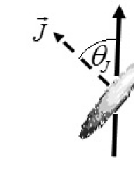
The projection of the molecular axis on the vertical -direction is given by:
| (4) |
where is the angle between and -axis, and is the angular frequency of molecular rotation.
By averaging Eq. (4) over time, we obtain:
| (5) |
For random and isotropic orientation of vector in space, the probability density for distribution is . The mean value of the deflection angle is then , where the constant presents the average deflection angle for an isotropic molecular ensemble:
| (6) |
Eq.(5) allows us to obtain the distribution function, for (and the related deflection angle) from the known isotropic distribution for . Since the inverse function is multivalued, one obtains
| (7) |
where we summed over the two branches of . This formula predicts an unimodal rainbow singularity in the distribution of the scattering angles at the maximal value (for ), and a flat step near the minimal one (for ). These results are similar to the ones derived by us previously for molecular scattering by oscillating optical fields [22].
As the next example, we consider the opposite case of polar molecules with and negligible polarization-type interaction. For the sake of simplicity, we start with a model, i.e. for a molecule that rotates with no azimuthal momentum. In the limit of ( is the rotational energy), the molecular axis is trapped by the electric field, and . As is increased, the molecules may still be trapped, but and for trapped molecules with high enough , . The latter happens because the molecules spend most of the time being against the electric field when performing nonlinear angular oscillations. As the energy is increased even more, the molecules become untrapped, and perform full rotations. In this case, we expect due to the same reason: the molecules accelerate their rotation when the dipole moment tends to be parallel to the electric field, and they decelerate it when the dipole moment looks against the field. As a result, the time-averaged value of is negative. Considering a molecular rotation in the presence of the electric field, we can write:
| (8) |
where is the moment of inertia. Assuming the untrapped regime (), the rotation period is given by [30]:
The time averaged value of is:
| (10) | |||||
Here ; and are the first and second order elliptic integrals, respectively. From Eq. (10) we learn that in the limit of weak fields, . This value is negative, as discussed above.
Summarizing, in the approximation, when , it is close to when , and it takes negative values in-between. This assumes the existence of a negative minimum of as a function of .
The properties of the quantity are somehow different in the considered model. For low , the molecular rotation is suppressed, and . The period of angular oscillations of the trapped molecules () is given by:
| (11) | |||||
The time-averaged value of is:
| (12) | |||||
where , and were defined above.
The function in Eq.(12) has a local minimum at , which suggests a rainbow peak in the distribution of in the case of a smooth distribution of the parameter . For high enough energy, the molecules rotate almost as free rotors, and we expect a rainbow peak in the distribution at , as was suggested by Eq.(7).
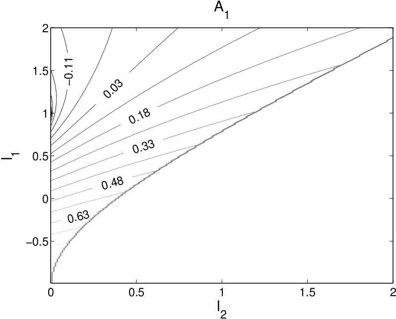
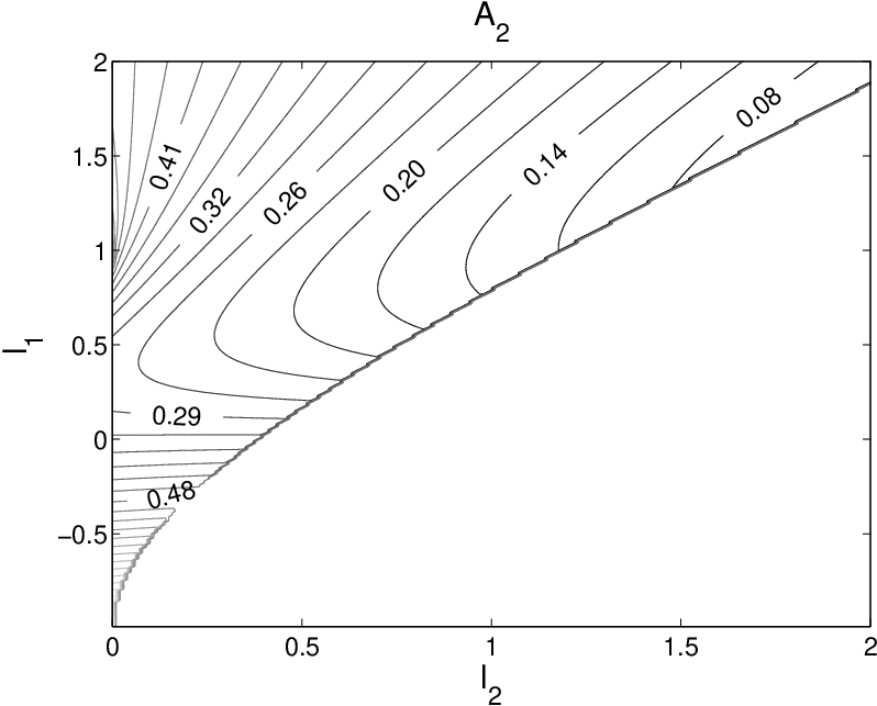
Finally, in order to complete our analysis, we consider the field-affected molecular rotation in case, find numerically and plot the quantities of (Figs. 3 and 4, respectively) for different values of dimensionless rotational energy and azimuthal canonical momentum (the details of the calculations can be found in the next section). For the lowest possible negative values of the total energy, both plots demonstrate angular trapping (). For small values of the azimuthal momentum we observe a negative shift (around ) of the maximum of , the nature of which has been already discussed. In this limit, we also observe a minimum at and a peak at , which is in agreement with the previous model. For high rotational energies (and high azimuthal momentum), . Finally, for high azimuthal momentum we observe also a strong decrease in the values, since the molecules mainly rotate in the plane in this limit.
III Classical Treatment
Consider a classical rigid rotor (linear molecule) described by the Lagrangian:
| (13) | |||||
where and are Euler angles, and is the moment of inertia. The canonical momentum for the angle
| (14) |
is a constant of motion as is a cyclic coordinate. The canonical momentum is given by
| (15) |
The Euler-Lagrange equation for the variable is
| (16) |
which leads to
| (17) |
When considering a thermal ensemble of molecules, it is convenient to switch to dimensionless variables, in which the canonical momenta are measured in the units of , with , where is the temperature [31], and is the Boltzmann’s constant. By setting , , and , Eq.(17) becomes:
| (18) |
where , and .
Considering a deflecting field that is adiabatically increasing to its final value (adiabatic with respect to the molecular rotational dynamics), we numerically solve Eq.(18) and find the time dependent values of and .
In order to find the , we calculate:
| (19) |
and consider as the limit value to which converges as . Here is the rising time in which the deflecting field reaches its maximal value .
The probability distribution of is given by:
| (20) | |||||
where
| (21) |
is the thermal distribution function.
Deflection of thermal molecules. Using this approach, we considered distribution functions for (and corresponding distributions of the deflection angle ) for a thermal beam of molecules. For the chosen rotational temperature , the typical ”thermal” value of the angular momentum is , where , is the rotational constant and is the speed of light. We plot the distribution functions for moderate () and strong () values of the deflecting field at Figs. 5 and 6, respectively. For the moderate field, and , so that the dipole-field interaction is comparable with the typical thermal rotational energy, while the polarization-type interaction is negligible. In this case, a sizable portion of molecules are trapped by the field, which is reflected in the high positive values of (Fig. 5a). The untrapped molecules are performing full rotations, and they contribute to the negative values of . Fig. 5b presents the distribution of , and it shows two rainbows (the first one at approximately , and the second one at ), as is expected from the discussion in the previous section. The distribution of the deflection angles (not shown here) is similar to the distribution of , as the contribution from the polarization-type interaction (proportional to ) is negligible in the considered numerical example. The distribution for the molecule may be directly measured in a deflection experiment that combines a homogeneous static field and an inhomogeneous laser field. The static field will define the distributins of and , and the laser field will deflect the molecules according to the values [22].

In the case of a strong field () shown at Fig. 6, , and is still negligible. Now the dominant portion of molecules is highly trapped by the electric field, and the distribution of is shifted accordingly to the higher positive values (Fig. 6a). The rainbow at in the distribution (Fig. 6b) practically disappears due to the increased amount of molecules with the suppressed rotation.

Finally, in Fig. 7 we present the case of a strong deflecting field, but at higher temperature. Though the field is as strong as in Fig. 6, value is similar to the one of Fig. 5, and the curves are correspondingly similar.

Deflection of pre-aligned molecules. Assume now that the molecules are subject to a femtosecond pre-aligning pulse polarized in -direction at , before they enter the deflecting field. The interaction of molecular permanent dipole moment with the laser pulse averages to zero because of the fast optical oscillations. The polarization-type interaction is given by the first term in Eq. (1), in which is replaced by the envelope of the femtosecond pulse, and an additional factor of is added due to the oscillatory nature of the optical field. We assume that the pulse is short compared to the rotational period of the molecules, and consider it as a delta-pulse. The rotational dynamics of the laser-kicked molecules is then described by the same formalism as above, but with replaced by
| (22) |
Here is a properly normalized kick strength of the laser pulse, with given by:
| (23) |
Here we assumed the vertical polarization (along -axis) of the pulse. Physically, the dimensionless kick strength, equals to the typical amount of angular momentum (in the units of ) supplied by the pulse to the molecule. For example, in the case of molecules, corresponds to the excitation by (FWHM) laser pulses with the maximal intensity of . The distribution functions for kicked molecules are shown in Fig. 8. The kick parallel to the deflecting field increases the rotational energy of the molecules (i.e. makes them untrapped), while keeping unchanged the value of the azimuthal momentum. As was explained in the previous section, untrapped molecules with relatively low azimuthal momentum contribute to the negative shift of the peak in the distribution function (Fig. 8a). Since most of the molecules became untrapped, the rainbow around in the distribution of becomes the dominant rainbow. For the numerical example under consideration, the distribution of the deflection angles has the same shape as the distribution for (with a proper scaling). As follows from Fig. 8a , a prealigning laser pulse applied parallel to the direction of the deflecting field leads to a dramatic narrowing in the distribution of the scattering angles, and increases the brightness of the molecular beam deflected by a static electric field.

In the case of an aligning pulse in the direction (perpendicular to the deflecting field), both and are replaced by:
| (24) |
The distribution functions for in this case are shown in Fig. 9.

Such a pulse forces the molecules to rotate preferentially in the planes containing the axis. In a previous work [22], we showed that the distribution of has two rainbows at and in the absence of the static field. In the present case, as can be seen from Fig. 9b, the distribution of still preserves the rainbow at , but the rainbow at is smeared due to the effect of the strong deflecting field (). Nevertheless, we still may observe a considerable concentration of molecules at low values. The peak at is still present due to the reasons explained in the previous section. The two rainbows are due to molecules that rotate with small azimuthal momentum. The distribution of (Fig. 9a) has now a strong peak at low positive values, since a great portion of the molecules is freely rotating with large azimuthal momentum provided by the laser kick.
Finally, before proceeding to the quantum treatment of the same problem, we refer the reader to Sec. VI, in which an alternative approach to the classical calculation of is given by means of the formalism of adiabatic invariants.
IV Quantum Treatment
For a more quantitative treatment, involving analysis of the relative role of the quantum and thermal effects on one hand, and the strength of the pre-aligning pulses on the other hand, we consider quantum-mechanically the deflection of a linear molecule described by the Hamiltonian:
| (25) |
where is the angular momentum operator.
Without the electric field , the eigenfunctions of the free-space molecule are given by the free-rotor eigenfunctions . Before the molecules enter the deflecting field, we prealign them by a short femtosecond laser pulse. Such a pulse creates a rotational wave packet of the states. After the prealigning laser pulse is over, the molecules enter adiabatically the region of the static field. Then, each state (within the wave packet) transforms into the corresponding eigenstate , where is the quantum number associated adiabatically with the quantum number . The relation between and the free-rotor eigenfunctions may be described by:
| (26) |
The force, acting on the molecule is given by:
| (27) |
The first derivative is obtained by the means of the Hellman-Feyman theorem, that is being in an eigenstate ,
| (28) |
From Eqs. (25), (27) and (28) it is clear that the deflection angle of a molecule in a state is given by Eq. (3), in which are replaced by:
| (29) |
In the quantum case, the continuous distribution of the angles is replaced by a set of discrete lines, each of them weighted by the thermal population of the state . Fig. 10 shows the distributions of in the thermal case (i.e. without prealignment). These results can be compared to their classical analogs in Fig. 7, where the same structure is seen.

If the molecules are subject to a strong femtosecond pre-aligning pulse parallel to the deflecting field, the corresponding interaction potential is given, as in the previous section, by Eq. (1), in which is replaced by the envelope of the femtosecond pulse (including the factor, as was explained in the previous section). If the pulse is short compared to the typical periods of molecular rotation, it may be again considered as a delta-pulse. In the impulsive approximation, one obtains the following relation between the angular wavefunction before and after the pulse applied at [31]:
| (30) |
where the kick strength, is given by Eq.(23). For the vertical polarization of the laser field, is a conserved quantum number. This allows us to consider the excitation of the states with different initial values separately. In order to find for any initial state, we introduce an artificial parameter that will be assigned the value at the end of the calculations, and define
| (31) |
By differentiating both sides of Eq.(31) with respect to , we obtain the following set of differential equations for the coefficients :
| (32) |
where . The matrix elements in Eq.(32) can be found using recurrence relations for the spherical harmonics [32]. Since and (see Eq.(31)), we solve numerically this set of equations from to , and find . In order to consider the effect of the field-free alignment at thermal conditions, we repeated this procedure for every initial state. To find the modified population of the states, the corresponding contributions from different initial states were summed together weighted with the Boltzmann’s statistical factors:
| (33) | |||||
where are the coefficients (from Eq. 32) of the wave packet that was excited from the initial state ; is the Kronecker delta symbol, and is the rotational partition function. The distribution in the case of parallel pre-alignment is given in Fig. 11. The results are quite similar to the classical results from Fig. 8.

In the case of an aligning pulse in the direction, the operator in Eq.(30) becomes:
| (34) |
and a procedure similar to the described above is used to find the deflection distribution (one should pay attention that is no longer a conserved number during the operation of the pulse in the direction). The distribution for the case of perpendicular prealignment is given in Fig. 12. These results are similar to the classical predictions from Fig. 9.

V Discussion and Conclusions
In this work we considered molecular deflection by weak and strong inhomogeneous static electric fields. As the deflecting field is increased, it modifies the time-averaged alignment/orientation of the molecules. This affects the dipole force, and we have studied both classically and quantum mechanically the resulting deflection process. We found that laser induced field-free pre-alignment provides an effective tool for controlling molecular deflection. Depending on the polarization of prealignment pulse, different control actions may be exerted. In particaular, we predict a dramatic increase in the brightness of the scattered molecular beam, when the prealignment pulse is parallel to the direction of the deflecting field. Though we discussed (for simplicity) linear molecules in this work, a similar control mechanism may be considered for polyatomic molecules with more complicated geometry. Being in free space such molecules rotate about their own axis as well, which leads to distribution different from that of Eq. (7), and is not necessarily . For such molecules the prealignment will play a significant role in reducing their dipole interaction with the static field. Molecular deflection by inhomogeneous static electric fields may be used for the separation of molecular mixtures. Narrowing the distribution of the scattering angles may substantially increase the efficiency of separation of multi-component beams, especially when the pre-alignment is applied selectively to certain molecular species, such as isotopes [33], or nuclear spin isomers [34, 35]. Controlling molecular deflection by means of laser-induced prealignment may be implemented also for magnetic molecules moving in the static inhomogeneous magnetic fields, and this phenomenon is a subject of the currently ongoing research. Controlling the dipole interaction by laser-induced pre-alignment may find applications in molecular deceleration methods using time and spatially varying electric and magnetic fields [36].
We acknowledge the support of our study by a grant from the Israel Science Foundation. This research is made possible in part by the historic generosity of the Harold Perlman Family. IA is an incumbent of the Patricia Elman Bildner Professorial Chair.
VI Appendix: Calculation of by means of the theory of adiabatic invariants
The energy of a molecule participating in the deflection process is:
| (35) |
where we neglected the effect of polarizability (which is small for the fields and molecules considered in the main body of the paper). The conjugate momenta and are given by Eqs.(14) and (15), respectively, and is a constant of motion. It is convenient to change variables and to define new constants [37, 38]:
| (36) |
| (37) |
| (38) |
It is easy to show that obeys the following equation:
| (39) |
which gives:
| (40) |
where is the rhs of the Eq.(39). If , the polynomial has two roots, such that . When , has three roots (denoted by ). Let us analyze the behavior of this polynomial. If , then . If we substitute , then . That means that the three real roots of are ordered as . The polynomial is positive between and , and each root corresponds to a real angle . This allows one to determine the half-period of the motion in the static field by integrating Eq.(40) from to .
Since the potential is time-dependent (at least during the rising time), the energy of the system is not a constant of motion. However, the deflection potential is adiabatic with respect to the rotational motion and, therefore, we can use adiabatic invariants to determine the energy of the system [37, 38, 39]. The adiabatic invariant related to the coordinate is:
| (41) |
From Eqs.(15), (39) and (41) it is easy to derive:
| (42) |
where is a constant. The energy of the molecule as a function of the energy without electric field is obtained numerically by solving the following equation:
| (43) |
where is calculated for , that is in the absence of the external field.
Once the energy of the system and the polynomial are found, is given by:
| (44) |
This is equivalent to calculating with the help of Eq.(19).
References
- [1] T. J. McCarthy, M. T. Timko and D. R. Herschbach, J. Chem. Phys. 125, 133501 (2006).
- [2] E. Benichou, A. R. Allouche, R. Antoine, M. Aubert-Frecon, M. Bourgoin, M. Broyer, Ph. Dugourd, G. Hadinger and D. Rayane, Eur. Phys. J. D. 10, 233 (2000).
- [3] H. J. Loesch, Chem. Phys. 207, 427 (1996).
- [4] R. Antoine, D. Rayane, A. R. Allouche, M. Aubert-Frecon, E. Benichou, F. W. Dalby, Ph. Dugourd, M. Broyer and C. Guet, J. Chem. Phys. 110, 5568 (1999).
- [5] H. Stapelfeldt, H. Sakai, E. Constant and P. B. Corkum, Phys. Rev. Lett. 79, 2787 (1997); H. Sakai, A. Tarasevitch, J. Danilov, H. Stapelfeldt, R. W. Yip, C. Ellert, E. Constant and P. B. Corkum, Phys. Rev. A, 57, 2794 (1998).
- [6] B. S. Zhao, H. S. Chung, K. Cho, S. H. Lee, S. Hwang, J. Yu, Y. H. Ahn, J. Y. Sohn, D. S. Kim, W. K. Kang, and D. S. Chung, Phys. Rev. Lett. 85, 2705 (2000); H. S. Chung, B. S. Zhao, S. H. Lee, S. Hwang, K. Cho, S. H. Shim, S. M. Lim, W. K. Kang and D. S. Chung, J. Chem. Phys. 114, 8293 (2001).
- [7] B. S. Zhao, S. H. Lee, H. S. Chung, S. Hwang, W. K. Kang, B. Friedrich and D. S. Chung, J. Chem. Phys. 119, 8905 (2003).
- [8] B. Friedrich, Phys. Rev. A 61, 025403 (2000).
- [9] R. J. Gordon, L. Zhu, W. A. Schroeder and T. Seideman, J. Appl. Phys. 94, 669 (2003).
- [10] R. Fulton, A. I. Bishop and P. F. Barker, Phys. Rev. Lett. 93 243004 (2004).
- [11] R. Fulton, A. I. Bishop, M. N. Schneider, P. F. Barker, Nature Phys. 2, 465 (2006).
- [12] T. Seideman, J. Chem. Phys. 106, 2881 (1997);J. Chem. Phys. 107, 10420 (1997); J. Chem. Phys. 111, 4397 (1999).
- [13] T. L Story and A. J. Hebert, J. Chem. Phys. 64, 855 (1976).
- [14] R. Schäfer, S. Schlecht, J. Woenckhaus and J. A. Becker, Phys. Rev. Lett. 76, 471 (1996).
- [15] P. R. Brooks, E. M. Jones and K. Smith, J. Chem. Phys. 51, 3073 (1969).
- [16] K. H. Kramer and R. B. Bernstein, J. Chem. Phys. 42, 767 (1965).
- [17] A. Lübbert, G. Rotzoll and F. Günther, J. Chem. Phys. 69, 5174 (1978).
- [18] L. Holmegaard, J. H. Nielsen, I. Nevo and H. Stapelfeldt, Phys. Rev. Lett. 102, 023001 (2009); F. Filsinger, J. Küpper, G. Meijer, L. Holmegaard, J. H. Nielsen, I. Nevo, J. L. Hansen and H. Stapelfeldt, J. Chem. Phys. 131, 064309 (2009).
- [19] B. A. Zon and B. G. Katsnelson, Zh. Eksp. Teor. Fiz. 69, 1166 (1975) [Sov. Phys. JETP 42, 595 (1975)].
- [20] B. Friedrich and D. Herschbach, Phys. Rev. Lett. 74, 4623 (1995); J. Chem. Phys. 111, 6157 (1999).
- [21] S.M. Purcell and P.F. Barker, Phys. Rev. Lett. 103, 153001 (2009).
- [22] E. Gershnabel and I. Sh. Averbukh, Phys. Rev. Lett. 104, 153001 (2010); Phys. Rev. A 82, 033401 (2010).
- [23] H. Stapelfeldt and T. Seideman, Rev. Mod. Phys. 75, 543 (2003).
- [24] V. Kumarappan, S. S. Viftrup, L. Holmegaard, C. Z. Bisgaard and H. Stapelfeldt, Phys. Scr. 76, C63 (2007).
- [25] J. J. Larsen, K. Hald, N. Bjerre and H. Stapelfeldt, Phys. Rev. Lett. 85, 2470 (2000).
- [26] J.G. Underwood, B. J. Sussman and A. Stolow, Phys. Rev. Lett. 94, 143002 (2005); K. F. Lee, D. M. Villeneuve, P. B. Corkum, A. Stolow and J. G. Underwood, Phys. Rev. Lett. 97, 173001 (2006).
- [27] S. S. Viftrup, V. Kumarappan, S. Trippe and H. Stapelfeldt, Phys. Rev. Lett. 99, 143602 (2007).
- [28] G. Tikhonov, K. Wong, V. Kasperovich and V. V. Kresin, Rev. Sc. Instr. 73, 1204 (2002).
- [29] N.F. Ramsey, Molecular Beams (Oxford University Press, New York, 1956)
- [30] I. S. Gradshteyn and I. M. Ryzhik, , , , 7th ed. (Elsevier Academic Press, USA, 2007).
- [31] E. Gershnabel, I. Sh. Averbukh and R. J. Gordon, Phys. Rev. A, 74, 053414 (2006).
- [32] George B. Arfken, Hans J. Weber, , 6th ed. (Elsevier Academic Press, USA, 2005).
- [33] S. Fleischer, I. Sh. Averbukh and Y. Prior, Phys. Rev. A 74, 041403(R) (2006).
- [34] M. Renard, E. Hertz, B. Lavorel, and O. Faucher, Phys. Rev. A 69, 043401 (2004).
- [35] S. Fleischer, I. Sh. Averbukh, and Y. Prior, Phys. Rev. Lett., 99, 093002 (2007); E. Gershnabel and I. Sh. Averbukh, Phys. Rev. A, 78, 063416 (2008).
- [36] J. A. Maddi, T. P. Dinneen and H. Gould, Phys. Rev. A, 60, 3882 (1999); E. Narevicius, C. G. Parthey, A. Libson, M. F. Riedel, U. Even and M. G. Raizen, New J. Phys., 9, 96 (2007).
- [37] P. Dugourd, I. Compagnon, F. Lepine, R. Antoine, D. Rayane and M. Broyer, Chem. Phys. Lett. 336, 511 (2001).
- [38] H. Goldstein, C. Poole and J. Safko, , 3rd ed. (Addison Wesley, USA, 2001).
- [39] L. D. Landau and E. M. Lifshitz, , 3rd ed. (Butterworth-Heinemann, UK, 1976).