VARIATIONAL APPROACH FOR THE ELECTRONIC STRUCTURE CALCULATION ON THE SECOND-ORDER REDUCED DENSITY MATRICES AND THE -REPRESENTABILITY PROBLEM
Abstract
The reduced-density-matrix method is a promising candidate for the next generation electronic structure calculation method; it is equivalent to solve the Schrödinger equation for the ground state. The number of variables is the same as a four electron system and constant regardless of the electrons in the system. Thus many researchers have been dreaming of this much simpler method for quantum mechanics. In this chapter, we give a overview of the reduced-density-matrix method; details of the theories, methods, history, and some new computational results. Typically, the results are comparable to the CCSD(T) which is a sophisticated traditional approach in quantum chemistry.
I Introduction
Chemistry is an important branch of science which treats change of matter. It explains, for example, why and how a protein works, the process converts to , etc. The goal is to predict, understand, and control what will happen when we mix some substances. To do that, we usually do experiments which can be explosive, poisonous, expensive and unstable. Therefore, it is desirable to do chemistry without experiments. Fortunately, the basic equation for chemistry is already known and it is called the Schrödinger equation [12]. It is possible to approximately solve the Schrödinger equation using computers with various methods and algorithms. Such branch of chemistry is called quantum chemistry and it is our main interest11 1 also known as theoretical chemistry or computational chemistry..
Determining the exact or approximate solution to the Schrödinger equation is the fundamental problem in quantum chemistry. This solution is called the wavefunction, or sometimes referred as electronic structure. If we know the electronic structure, we can do chemistry. Often such methods are referred as ab initio (Latin word which means “from the beginning”) or the first principle method if approximations are not heuristic or do not employ parameters from experiments.
The ground state energy calculation of a non-relativistic and time-independent, -electron molecular system under the Born-Oppenheimer approximation is the most important problem [57]. It can be obtained as the lowest eigenvalue of the electronic Schrödinger equation:
| (1) |
where is the Schrödinger operator or Hamiltonian defined by
| (2) |
in which is the atomic number of the nucleus , is the distance between the electron and nucleus , and is the distance between two distinct electrons. The solution of (1), in , with the inner product ( includes integration over spin variables), is the wavefunction, and the corresponding eigenvalue , the total energy of the system.
Besides, since electrons are fermions, the wavefunction itself is antisymmetric due to Pauli exclusion principle:
That is to say, we must solve the Schrödinger equation in the antisymmetric subspace of . We denote such space as .
Even on computers, treating the -particle wavefunction is very difficult. Thus, we discretize the Hilbert space by taking antisymmetric products of the one-particle Hilbert space , whose complete orthonormal system (CONS) is . Each is called single-electron wavefunctions or spin orbitals
| (3) |
We can explicitly construct a CONS of using by the Slater determinants defined as follows [57]:
Here, we used an ordered set of indices . It is known that is a CONS of [33].
A second approximation to solve the Schrödinger equation would be choose carefully functions from a CONS by chemical or physical intuition. Then we construct a subspace of by the Slater determinants considering all possible combinations of spin orbitals among possibilities. In this case, solving the Schrödinger equation becomes the eigenvalue problem of the Hamiltonian matrix which now seems to be feasible on computers. Nevertheless, the dimension of the problem becomes which obviously is impractical even for small values. The (approximate) ground state energy obtained by this procedure is considered the reference value, and called Full Configuration Iteration (Full CI) (energy). The mainstream approaches in quantum chemistry can be roughly interpreted as linear or nonlinear approximations of this eigenvalue problem, e.g., Hartree-Fock method, second-order perturbation methods, coupled cluster methods, truncated CI methods, etc.
Our main motivation is employ the second-order reduced density matrix (2-RDM) as the basic variable for quantum mechanics to construct simpler methods. Since only two-body interactions exist in nature, we can calculate all observables using the 2-RDM. Moreover, the number of variables of the 2-RDM is always four, regardless of the number of electrons in the system ( when discretized), whereas the wavefunction scales like ( when discretized).
This chapter is organized as follows. In Section 2, we define the first-order and second-order reduced density matrices, and introduce the notion of -representability and its conditions. The reduced-density-matrix method is a viable implementation to approximate the ground state energy of molecular systems. The reduced-density-matrix method is formulated as an semidefinite program in Section 3, and its numerical results using a parallel optimization code is given in Section 5. In Section 4, we give a brief historical note of this approach. Finally in Section 6, we give some concluding remarks.
II The Reduced-Density-Matrix Method
II.1 Pure states and ensemble states
Most generally, a quantum system containing particles is described by the density matrix which was introduced independently by von Neumann, Landau, and Bloch, and is an ensemble average of wavefunctions,
where , , and is a CONS of an -particle state. For a pure state where the system is described by the wavefunction , can be written by
This is equivalent to requiring to be idempotent; . Hereafter, when we refer to a state, it means be an ensemble if not otherwise specified. We are mainly interested in the pure state but usually we do not care about whether is a pure or ensemble. This only becomes a problem when the system is degenerated or we consider its subsystems.
II.2 The first-order and second-order reduced density matrices
Given an ensemble , the first-order Reduced Density Matrix (1-RDM) [12] is defined by
The second-order Reduced Density Matrix (2-RDM) [28, 33, 35] is given by
and higher-order RDMs are defined in an analogous way. The normalization factor for the -th order reduced density matrix is then . The second-quantized versions are defined using a set of creation and annihilation operators , where creates and annihilates a particle at of as follows [57]:
The normalization factor for the -th order reduced density matrix is for this case. The equivalence of these two different expressions can be found by
where we used the single-particle wave function of (3). The following conditions are inherited by these definitions:
-
(1) the 1-RDM and 2-RDM are Hermitian,
-
(2) the 2-RDM is antisymmetric,
-
(3) trace conditions are valid,
-
(4) a partial trace condition holds between the 1-RDM and 2-RDM,
Additionally, we can find more conditions from the symmetry of the system. In particular, the spin symmetry of the (ground state) molecular systems is important and formulated as follows:
-
(5) the total spin ; the 2-RDM should be the eigenstate of spin operator
where is defined as follows:
The indices , means that we choose spin eigenfunctions of the -axis for , and reorder them so that means -th spacial function and , denote eigenfunctions of -spin and -spin; , respectively.
-
(6) The -component of the spin, can be chosen as integer or half integer,
In the subsequent discussion, one will notice that the 1-RDM can be disregarded throughout. However, we explicitly use it in order to prioritize the compactness of the notation.
II.3 Solving the ground state problem using 1- and 2-RDMs
The Hamiltonian of the most general form in second-quantization can be written by:
where and are one- and two-particle terms which can be calculated from the molecular Hamiltonian (2) by the Slater’s rule as follows:
where is the distance between an electron and a nucleus. Then, the total energy can be expressed using as follows:
The ground state energy can be calculated minimizing the total energy over 1- and 2-RDMs.
| (4) | |||||
| (5) |
It is easy to show that this minimization (4) is equivalent to solve the Schrödinger equation for the ground state, and often such kind of methods are called variational methods. Moreover, (5) is also equivalent to solve the Schrödinger equation for the ground state. Advantage of using 1- and 2-RDMs instead of is that the number of variables are reduced drastically.
II.4 The -representability problem and the -representability conditions
In 1950’s, researchers based on the above facts chose the 1- and 2-RDMs as basic variables, and did some variational calculations; according to Löwdin [34], F. London, J. E. Mayer, A. J. Coleman, P. O. Löwdin, R. McWeeny, N. A. March, C. A. Coulson and others have attempt to minimize via (5). However, their results were considerably lower than the true energy. The reason is that the trial 2-RDMs were not actually derived from an existing density matrix . We need some more conditions on the trial 2-RDM to ensure that it comes from a true . Such formalism of the problem was first described by A. J. Coleman in 1963 and named -representability problem, and these conditions are known to be the -representability conditions [9]; Given a trial -th order RDM , if there exists some wavefunction or ensemble which reduces to the -th order RDM , then this is pure or ensemble -representable, respectively.
II.5 On the complete -representability conditions
Given a 1- and 2-RDM, they should satisfy the relations to of Section 2.2 The 1- and 2-RDM for the ground state should additionally satisfy and . Therefore, these conditions are necessary conditions for the -representability. Unfortunately, these conditions are not sufficient, thus early attempts failed and obtained very low energy. The necessary and sufficient condition for the 1-RDM is relatively easy [30, 9]. However, the complete (sufficient) -representability of the 2-RDM is very complicated in general. Garrod and Percus [26] showed that the 2-RDM is ensemble -representable if and only if
where is every possible Hamiltonian and is the ground state energy corresponds to . Thus, the ensemble -representable set can be defined by:
This result is theoretical and very important, but totally not practical since if one wants to calculate the exact ground state energy of a Hamiltonian, then he/she must know the exact ground state energy of the system beforehand. This is a tautology! After that, many researchers seek the complete -representability condition, and did not succeed. A meaningful result from complexity theory was obtained by Liu et al. [32] in 2007. They showed that the computational complexity of the -representability problem is QMA-complete, which is the quantum generalization of NP-completeness. Thus it is almost hopeless to find an efficient algorithm to decide whether a given 2-RDM is -representable or not. We can consider a more physical example: the ground state problem of the spin-glass Hamiltonian is known to be a very hard problem, and equivalent to solve the max-cut problem or the traveling sales person problem, which in turn are known to be NP-hard [3]. If the complete -representability conditions were easy to handle, we could solve such difficult problems in computer science as well. Currently we do not know how to solve these problems efficiently. We just want to stress, the complete -representability is a really hard problem.
II.6 Formulating as a variational problem, and its geometrical representation
The problem we want to solve can be formulated using the 1- and 2-RDMs as basic variables,
is known to be a compact convex set. Besides, all possible Hamiltonians and the corresponding ground state energies serves as a characterization of this convex set. To be more precise, a 2-RDM corresponding to the ground state of an -particle Hamiltonian is a surface point, and any surface point of corresponds to the ground state of some Hamiltonian [53]. The compact and convex set of the -representable set is represented as an ellipse (we do not show, but there are also cusp points as well) in Fig. 1. The Hamiltonians , , , and , and their ground state energies , , , and serves as -representability conditions, respectively.

II.7 Some known necessary -representability conditions
We should not be demotivated by the facts of the previous subsection. Understanding the chemical and/or physical meaning of the necessary -representability conditions is much more important. Mathematical theorems do not tell about chemistry or physics. In practice, -representability conditions for the molecular systems might not be so difficult.
We seek for chemically and/or physically meaningful necessary -representability conditions on the 1- and 2-RDMs. The necessary and sufficient conditions for an ensemble -representability for the 1-RDM is characterized by its eigenvalues lying between 0 and 1 [30, 9]. For the pure state, it is more complicated [1]. Coleman introduced two necessary conditions called the and conditions [9]. These conditions require the positive semidefiniteness of the -matrix (), and the -matrix
| (6) | |||||
| (7) |
Another important necessary condition is called the condition [26], which also require positive semidefiniteness of the -matrix defined as follows
| (8) |
In the original paper by Garrod-Percus, the definition of the -matrix is non-linear:
| (9) |
but for a fixed particle state, these -matrices share the same eigenvalues, since can be replaced with [16]. In Zhao et al [67], we can find explicitly formula of and conditions from Erdahl’s survey paper [14]:
| (10) | |||||
| (11) |
which are stronger conditions. An important property of these matrices is that , , and -matrices can be written only by linear combinations of the 2-RDM elements like following:
where is the antisymmetrizer operator acting on an arbitrary function ,
For and ’s cases, the 3-RDM terms cancel out. The condition replaces the condition and is slightly strengthened by the addition of the one-particle operator [5, 40].
Other positive semidefinite type representability conditions are known such as the and . However, they are implied by the condition [31].
We can extend these conditions to positive semidefiniteness of higher order RDMs. These extensions seems to be known for a long time. Erdahl and Jin [17] formulated the -th order approximation to the -particle density matrix in terms of the semidefiniteness conditions on the -th order RDMs, which is an generalization of the , , , and conditions.
II.8 The reduced-density-matrix method
We call as the reduced-density-matrix method, the variational method having the 2-RDM (and the 1-RDM) as the basic variable(s) restricted to some approximation of the -representability set . It can be formulated as follows:
| (12) |
Among the possibilities, we usually consider the set obtained by imposing some necessary conditions for the -representability. The set should satisfy the following properties.
- •
satisfies some necessary conditions of ensemble -representability.
- •
compact set, so that a linear functional (the Hamiltonian) has a minimum.
- •
convex set, so that the solution would not be stuck into local minima.
- •
stringent, so that resultant 2-RDM should be physically or chemically meaningful.
- •
computationally feasible and/or efficient.
- •
completely general: since the form of the Hamiltonian is totally general, it is not only applicable to chemistry but also to physics.
- •
ab initio: no empirical parameters. Currently very successful methods based on the density functional theories employ a lot of empirical parameters.
We can find new -representability conditions from chemical or physical requirements satisfying the above properties by constructing a Hamiltonian and obtaining an upper bound to the ground state energy. Then we can add this as a new condition. These “cuts” may strengthen .
Trivial -representability conditions with the , , , and conditions and every possible combination of the , , , , and conditions, satisfy the above criteria. These variational energies have the following property:
- •
If we add more necessary conditions, the calculated energy usually becomes better and would never become worse:
where is the variational energy with the and conditions, is the variational energy with the , , , and conditions, etc. (see Fig 2). This property is totally opposite from traditional wavefunction approaches. Variational calculation using the wavefunction gives upper bounds, and approximation to the total energy becomes lower (better) when the variational space becomes larger .
Note that the obtained 2-RDM may not be unique, even when the original problem is non-degenerated and the energy is unique.

II.9 Some interpretations on conditions
We usually enforce only the necessary conditions on the trial 2-RDMs. Therefore, the RDM method gives lower bounds to the exact energy, an -representable 1-RDM and a non-physical 2-RDMs. Thus it is important to realize the physical meaning of the necessary conditions employed in the calculations. The following results may be useful to interpret results from actual calculations on molecules and atoms:
-
(a) If a trial 2-RDM satisfies the and conditions, the original 2-RDM is ensemble -representable [9].
-
(b) If a trial 2-RDM satisfies the condition, then 1-RDM from the original 2-RDM is ensemble -representable [42].
-
(c) If the Hamiltonian of a system is time-reversal invariant, and the number of particles , is even, the necessary and sufficient condition that an approximate 1-RDM corresponding to a non-degenerate energy eigenstate be -representable is that its natural spin-orbital occupation numbers be equal in pairs [56]. Moreover Coleman proved that the AGP (anti-symmetrized power) wavefunctions covers all such 1-RDMs [10]. Thus if these conditions apply to the systems, we always obtain pure representable 1-RDMs with necessary -representability conditions.
-
(e) The condition is exact at the high-correlation limit for the Hubbard model, since the two particle term of the model (, where , is the number of sites, is the -th site, and and denote up-spin and down-spin of the electrons, respectively) is a -type Hamiltonian (), which is bounded by zero [64].
III Formulation of the RDM method’s Problem as an Semidefinite Program and its Solution by the Interior-Point Method
III.1 Semidefinite program
Semidefinite program (SDP) has established as an important class of problems in optimization since 1990’s. It is known to have an elegant mathematical theory, and an efficient algorithm called interior-point method which can solve it in polynomial-time complexity. Refer for instance to [58] for a nice survey about SDPs.
Let be given block-diagonal real symmetric matrices with prescribed block sizes, and be given real vectors. We denote by a diagonal matrix with the elements of the vector on its diagonal.
An SDP is defined for instance by
| (13) |
where we refer it as the primal SDP. The notation means that is symmetric positive semidefinite. Then, we can define the dual SDP as
| (14) |
The variables for the primal SDP is while for the dual SDP is . Under mild assumptions22 2 to be more precise, we need to eliminate some variables using the equalities , and assume the Slater’s condition, but we avoid to do it here to be cumbersome. [58], the solution of (13-14) should satisfy
| (15) |
These conditions are equivalent to earlier result by Erdahl [15] and Bellman and Fan [4].
The advantage of considering the variables in the primal and dual SDPs simultaneously is that we can check the numerical correctness of the approximate solution from the above relations.
III.2 Formulation of the RDM method’s problem as an SDP
Hereafter, we assume that we have chosen spin orbitals from (3), which is assumed to give a good approximation for the desired wavefunction we seek. There are plenty of these bases in quantum chemistry, and we actually use them on the numerical experiments which follows. Also, notice that all definitions and notions of -representability and its conditions can be defined accordingly using this finite basis of CONS.
The RDM method’s problem imposing some necessary -representability conditions such as the (6), (7), (8), (10), (11) or conditions, is in fact an SDP. In order to make its formulation more clear, we perform some linear transformations on the matrices involved in the problem. In (12), the 1-RDM variable , and the corresponding Hamiltonian have two indexes, which correspond to ordinary matrices in linear algebra. However, the other matrices involved in the calculations have four or even six indices each. To convert from these notations convenient for quantum chemists to the notation of elementary linear algebra, we need to map each pair or triple of indices to a composite index on these matrices. For instance, the 2-RDM element will be mapped to , which results in a symmetric matrix of size . We assume henceforth that all matrices are transformed to become two-index matrices, and we keep the same notation as before for simplicity. Furthermore, due to spin symmetry [67], all these matrices will reduce to block-diagonal matrices of sizes specified in Table 1 [22, 23] 33 3 There is an additional term in the column of of Table II [23], which is missing and corresponds to the size or the 1-RDM..
| -repres. cond. | size of block matrices |
|---|---|
| (2 blocks) | |
| (2 blocks) | |
| condition | (1 block), (2 blocks) |
| condition | (1 block), (2 blocks) |
| condition | (1 block), (2 blocks) |
| condition | (2 blocks), (2 blocks) |
| condition | (2 blocks), (2 blocks) |
| condition | (2 blocks), (2 blocks) |
| in (14) | |
| in (14) | |
| here , for integers | |
Now, let us define a linear transformation svec: from the space of symmetric matrices . For ,
Then, defining , , and finding the suitable matrices and vectors for the corresponding necessary -representability conditions of Table 1, for instance, we can cast the problem (12) as (14).
Although these transformations and formulations seem a little confusing, it is in fact the formulation Garrod et al. arrived 35 years ago [24]. Nakata et al. [48, 46, 47] formulated the problem as the primal SDP (13) instead when they performed the first computation as an SDP. For a more detailed discussion about these transformations and the formulations, see for instance [67, 22, 23].
III.3 Theoretical computational complexity of the primal-dual interior-point method
As it was previously mentioned, SDPs can be solved in polynomial-time using interior-point methods [58]. In particular, employing the parallel code SDPARA [20], which is an implementation of the primal-dual interior-point method, one can theoretically expect that it will take iteration with floating-point operations per iteration. Here refers to the size of the largest block matrix in , is the maximum number of nonzero elements in each of these matrices, is the total number of available CPU cores in the parallel computer, and is the accuracy which we can expect when we replace the rhs of (15) “=0” by “” (where ). In our case, , , , and therefore, the total theoretical floating-point operations is [23].
IV Some Historical Remarks
Here we make an attempt to list some articles related to our work in chronological order. However, it is far from being complete.
The definition of the RDM was explicitly spelled out by Husimi [28] in 1940. The dependence of the energy on the 2-RDM (and 1-RDM) appeared in Löwdin [33] and Mayer [35] in 1955. The necessary and sufficient conditions for an ensemble 1-RDM, i.e., , tr, were obtained by Kuhn [30] in 1960 and Coleman [9] in 1963. In this latter article, the precise formulation of the -representability problem, the and conditions (for the 2-RDM) were also stated. In the next year, the condition was proposed by Garrod and Percus [26].
The restriction of the -representability problem only on the diagonal elements of the 2-RDM, known as the diagonal problem, were investigated by Weinhold and Wilson [63], Davidson [11], McRae-Davidson [41], and Yoseloff [66] since late 1960’s. Other progresses on this topic can be found in the survey [2].
The first variational calculation on the 2-RDM imposing the necessary -representability conditions for the doubly ionized carbon C++ were performed by Kijewski and co-authors since late 1960’s [29] (see earlier reference therein). Garrod and co-authors proposed several algorithms, some of them which resemble modern optimization algorithms, and reported results for the beryllium () [25, 54, 24]. In particular, Mihailović and Rosina applied it to nuclear physics [43], but obtained large deviations to the full CI calculations if compared to electronic systems.
In the 1978 survey paper of Erdahl [14], we can find the conditions which is knows as , [67], and conditions [5, 40]. He also proposed algorithms based on the exact mathematical characterization of solutions of the lower bound method (RDM method) in the next year [15].
These were the golden ages for the RDM research, but somehow faded away because it was realized soon that the underlying problem is computationally difficult and poor results were obtained for nuclear systems.
A revival of the 2-RDM approach appeared since 1992 due to Valdemoro [59], Nakatsuji and Yasuda [51], and Mazziotti [36]. This approach is based on the density equation or the contracted Schrödinger equation (CSE), which is equivalent to solve the Schrödinger equation. Nakatsuji proved that if an -representable 4-RDM satisfies the CSE, then the original satisfies the Schrödinger equation and vice versa [50]. Valdemoro, Nakatsuji-Yasuda and Mazziotti consider the 2-RDM as the basic variable. The CSE requires 1- to 4-RDMs, thus they reconstruct 3- and 4-RDMs using 1- and 2-RDMs and solve the CSE iteratively. In this approach, they assume the resultant 2-RDM is nearly -representable because the reconstruction functional is physically relevant; they did not explicitly impose any -representability conditions. Their results are quite good, and can be compared to single and double CI for small atoms and molecules such as , , and . The absolute values of negative eigenvalues of the , , and -matrices were small. However, researchers payed little attention to this approach since non-convergence or divergence occur especially where the correlations are strong [13]. There are difficulties in systematic refinements of the reconstruction functional even though some improvements are reported [65], but there are even more miscellaneous problems [52].
In 2001, Nakata et al. [48] were the first to employ an optimization software to solve the RDM method’s problem as an SDP, and reported computational results imposing the , , and conditions on a series of small atoms and molecules. The results were better than the SDCI calculations, and obtained correlation energies from 100% to 120%. As mentioned in Section III.1, these results have a numerical certificate of correctness, which could not be obtained before the advent of interior-point methods. Also, the numerical convergence does not depend on the initial guess as it is common in Hartree-Fock, CCSD methods, etc. Moreover, there exists a global minimum, whereas this is not guaranteed in the CSE approach for instance. In the next year, Nakata et al. [46] showed results for the dissociation limit for several molecules including triple bonded , demonstrating numerically that the RDM method do not break down as the single reference methods such as CCSD and perturbation methods. However, it was also shown that size consistency is slightly deviated.
The inclusion of the Weinhold-Wilson inequalities [63], which was not satisfied only including the , , and conditions [46], however showed little progress in the results [47].
In 2002, Mazziotti immediately reproduced Nakata et al.’s results and applied to diatomic molecules [37]. The prolific research by Mazziotti and his colleagues in the following years [40] corroborated with these results.
In 2004, a breakthrough was done by Zhao et al. They included additionally the and conditions, which became very strong conditions for small molecules and atoms. They noted a “spectacular increase in accuracy” and results were comparable to CCSD(T); typically the correlation energies for various atoms and molecules were between 100% to 101% [67, 22, 45].
In the same year, Mazziotti announced the RRSDP method [38] in which he reformulates the SDP problem as an nonlinear and nonconvex problem and applies a quasi-Newton method to solve it [6]. In 2006, Cancès et al. proposed and implemented the dual problem of (12) [7].
Applications to the one-dimensional Hubbard model was done by Hammond et al. [27]. They calculated the Hubbard models with , , , and conditions up to 14 sites. The obtained error per site was for ’s case with , , , and conditions for , when correlation is strongest. Nakata et al. investigated the high correlation limit using multiple-precision arithmetic version of SDP solver, called the SDPA-GMP [45]. At the high correlation limit, they reproduced the exact energy and proved that the condition is exact [64].
The size-consistency and size-extensivity are important properties when the size of the systems becomes bigger or larger. Nakata et al. found slight deviations [46], but Van Aggelen et al. showed very clear and systematic examples that the RDM method gives incorrect dissociation limit with fractional charges on the well-separated atoms of diatomic molecules with , and conditions. For the ’s case, the Mulliken populations were 5.98 and 8.00 at the dissociation limit. Even adding and conditions they did not fix the problem [60, 61]. Nakata and Yasuda investigated numerically that size-extensivity is also slightly violated by calculating 32 non-interacting and [49]. The inextensive contributions to energies are and a.u. using the STO-6G basis set, respectively. Later, Verstichel et al. also proposed a method to “cure” this pathological behaviour of the RDM method, however quite demanding [62]. Currently solutions to size-consistency is not practical.
V Numerical Results for the RDM Method
Here, we give numerical results we obtained so far for the RDM method imposing some necessary -representability conditions. Some of them are completely new.
V.1 New numerical results for larger systems
We present here some numerical results for the largest systems solved so far by our group.
The SDPs obtained by the RDM method imposing the , , or , , , , conditions were solved using the parallel code SDPARA 7.3.2 [20, 21]. The calculations were performed at the Kyoto University’s T2K supercomputer using 128 nodes, were each node has 4 CPUs (quad-core AMD Opteron 8356 2.3GHz) and 32GB of memory, giving a total of 2048 cores; and at a self-made computer cluster using 16 nodes, were each node has 2 CPUs (quad-core Intel Xeon 5460 3.16GHz) and 48GB of memory, giving a total of 128 cores.
Table 2 shows the results for five molecules were or spin orbitals were used [21]. The full CI and SDCI (singly and doubly substituted configuration interaction) calculations were performed using the package Gamess [55], while CCSD(T) (coupled cluster singles and doubles with perturbational treatment of triples) and Hartree-Fock calculations were obtained by Gaussian98 [19]. The entries, excepting the full CI, give the ground state energy differences to the full CI. The RDM method always gives a energy lower than full CI, while SDCI and Hartree-Fock give higher. CCSD(T) usually results in higher energy, but not necessarily. Units are in Hartree. The acceptable accuracy in quantum chemistry is 1kcal/mol which corresponds to approximately 0.0016 Hartree. Also, the correlation energy is an important measure in quantum chemistry. It is defined as a percentage relative to the Hartree-Fock (0%) and full CI (100%):
where the energy calculated by the RDM method, CCSD(T) or SDCI.
| system | state | basis | ||||||||
|---|---|---|---|---|---|---|---|---|---|---|
| NH | double- | 28 | 10 (5) | 1 | 0.000 6 | 0.000 63 | 0.008 74 | 0.141 98 | 55.624 71 | |
| 100.4 | 99.55 | 93.84 | 0 | 100 | ||||||
| CH2 | double- | 28 | 8 (4) | 1 | 0.000 4 | 0.000 59 | 0.005 80 | 0.100 67 | 38.962 24 | |
| 100.4 | 99.42 | 94.24 | 0 | 100 | ||||||
| NH3 | valence double- | 30 | 10 (5) | 1 | 0.000 5 | 0.000 49 | 0.007 46 | 0.128 75 | 56.304 89 | |
| 100.4 | 99.62 | 94.45 | 0 | 100 | ||||||
| CH3 | valence double- | 30 | 9 (5) | 2 | 0.000 3 | 0.000 31 | 0.004 01 | 0.094 54 | 39.644 14 | |
| 100.3 | 99.67 | 95.75 | 0 | 100 | ||||||
| C2 | valence double- | 36 | 12 (6) | 1 | 0.003 5 | 0.000 39 | 0.055 98 | 0.285 66 | 75.642 11 | |
| 101.2 | 99.86 | 80.41 | 0 | 100 |
From Table 2, we can conclude that the RDM method imposing the conditions, gives equally better energies than CCSD(T) in absolute value. C2 molecule is exceptional, however, it is known to be a difficult system in quantum chemistry.
Table 3 shows the same result for the O molecule were spin orbitals were used. The full CI calculation was not possible for this case due to the size limit on the computer, and therefore, we restrict to show only the ground state energy corresponding for each entry.
| system | state | basis | |||||||
|---|---|---|---|---|---|---|---|---|---|
| O | double- | 40 | 15 (8) | 2 | 149.450 2 | 149.385 95 | 149.360 26 | 149.091 83 |
Table 4 shows the typical sizes of the problem when formulated as an SDP (see Section III.1), and the computational time to solve them by SDPARA 7.3.2 at the T2K supercomputer or at the computer cluster.
In the previous work [45], we only could solve the RDM method’s problem with conditions up to spin orbitals. Here, we give results up to . This achievement was possible due to a major update in the parallel code SDPARA 7.3.2 [20, 21]. It became faster, and now it can take advantage of multi-core (multi-thread) computation in addition to the ordinary MPI (message passing interface) computation.
| system | -repres. cond. | time (s) | system | CPU cores | |||
|---|---|---|---|---|---|---|---|
| NH | 28 | 27,888 | 4,032 | 27,949 | T2K | 2048 | |
| CH2 | 28 | 27,888 | 4,032 | 26,656 | T2K | 2048 | |
| NH3 | 30 | 36,795 | 4,965 | 72,026 | T2K | 2048 | |
| CH3 | 30 | 36,795 | 4,965 | 68,593 | T2K | 2048 | |
| C2 | 36 | 76,554 | 8,604 | 1,554,675 | c.c. | 128 | |
| O | 40 | 116,910 | 800 | 5,943 | T2K | 2048 |
For other physical properties such as the dipole moments, refer to [45].
V.2 Summary of the numerical experiments
We present a graphical summary of the data obtained in our previous work [45] with the addition of new ones presented in the previous section.
The ground state energy differences to full CI of the RDM method imposing the or , and of Hartree-Fock for the 57 atomic or molecular systems [45] and those 5 shown at Table 2 are plotted in Figure 3. Each horizontal bar corresponds to a system and they are ordered accordingly to the order it appears in the tables. That is, the lowest one corresponds to the Lithium atom with spin orbitals [45], while the upper 5 corresponds to the data of Table 2 (notice that we do not have the values for and entries for this case).

Apparently, it does not seems to exist an correlation between the Hartree-Fock and the RDM method’s results. However, we clearly notice that the imposing the conditions, we can obtain results much better than the Hartree-Fock’s ones.
Figure 4 shows the ground state energy differences to full CI of the RDM method imposing the (same value as Figure 3) or , and of CCSD(T) for the 57 atomic or molecular systems [45] and those 5 shown at Table 2 (notice that we do not have the values for entries for this case).
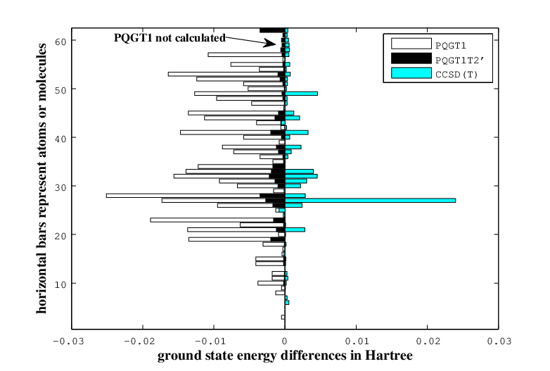
If you compare the RDM method with conditions and the CCSD(T) values, they seems equally good. However, in some case CCSD(T) can fails to converge. There are 4 case in [45] which are replaced by zero in Figure 4. The largest deviation of 0.00279 Hartree to full CI for CCSD(T) is for the Oxygen atom at the state [45].
VI Concluding Remarks
In this chapter, we showed the outline of the reduced-density-matrix method with applications to atomic and molecular fermionic systems. Some feature of this method are: (i) it is an ab initio method, which is rigorously the same as the Schrödinger equation for the ground state; (ii) the number of variables is always four, regardless of the size of the system; (iii) from the sparsity of the first- and second- order reduced density matrices the existence of a linear scaling method is apparent. The major obstacle for this method is the fundamentally difficulty of obtaining the complete -representability conditions for the 2-RDM. However we know fairly good approximated (necessary) condition like , , , and conditions which reproduces comparable ground state energies to CCSD(T), which is considered the golden standard method in quantum chemistry. The considered problem becomes a semidefinite programming problem, which minimizes a linear functional keeping the eigenvalues of matrices non-negative. In this chapter, we presented new results; , , , , , and using a supercomputer with a highly efficient semidefinite programming solver, SDPARA. The semidefinite programming problems for , , , and are the largest problems solved so far in the standard formulation. The correlation energies using , , , , for , , was , for was , and for was , respectively. For we used the double- basis, and attained of correlation energy since the open-shell systems are difficult and due to large space, we only employ the , and conditions.
We would like to close this chapter saying that the RDM method is a promising method for quantum chemistry or condensed matter physics. Developing the RDM method is important and fundamental to chemistry and physics.
Acknowledgments
The large-scale supercomputer computations for this research have been supported by the Collaborative Research Program for Large-Scale Computation of ACCMS and IIMC, Kyoto University. M. N. was supported by the Special Postdoctoral Researchers’ Program of RIKEN, and is partially supported by Grant-in-Aid for Scientific Research (B) 21300017. M. F. is very thankful for the invitation to the program “Complex Quantum Systems” held at the IMS-NUS, specially to the organizers Heinz Siedentop and Matthias Christandl. He also enjoyed the discussion with Prof. Robert Erdahl. M. F. is partially supported by Grant-in-Aid for Young Scientists (B) 21700008.
References
- [1] M. Altunbulak and A. Klyachko, “The Pauli principle revised”, Commun. Math. Phys., 282 (2008), 287–322.
- [2] P. W. Ayers and E. R. Davidson, “Linear inequalities for diagonal elements of density matrices”, in [39], 443–483.
- [3] F. Barahona, M. Grötschek, M. Jünger, and G. Reinelt, “An application of combinatorial optimization to statistical physics and circuit layout design”, Oper. Res., 36 (1988), 493–513.
- [4] R. Bellman and K. Fan, “On systems of linear inequalities in Hermitian matrix variables”, in Convexity, Vol. 7 of Proc. Sympos. Pure Math., American Mathematical Society, Providence, RI, 1963, 1–11.
- [5] B. J. Braams, J. K. Percus, and Z. Zhao, “The T1 and T2 representability conditions”, in [39], 93–101.
- [6] S. Burer and R. D. C. Monteiro, “A nonlinear programming algorithm for solving semidefinite programs via low-rank factorization”, Math. Program., 95 (2003), 329–357.
- [7] E. Cancès, G. Stoltz, and M. Lewin, “The electronic ground-state energy problem: A new reduced density matrix approach”, J. Chem. Phys., 125 (2006), 064101, 5 pages.
- [8] J. Cioslowski (ed.), Many-Electron Densities and Reduced Density Matrices, Kluwer Academic/Plenum Publishers, New York, 2000.
- [9] A. J. Coleman, “Structure of fermion density matrices”, Rev. Mod. Phys., 35 (1963), 668–689.
- [10] A. J. Coleman and V. I. Yukalov, Reduced Density Matrices: Coulson’s Challenge, Lecture Notes in Chemistry, Vol. 72, Springer, New York, 2000.
- [11] E. R. Davidson, “Linear inequalities for density matrices”, J. Math. Phys., 10 (1969), 725–734.
- [12] P. A. M. Dirac, “Quantum mechanics of many-electron systems”, Proc. Roy. Soc. (London), A 123 (1929), 714–733.
- [13] M. Ehara, M. Nakata, H. Kou, K. Yasuda, and H. Nakatsuji, “Direct determination of the density matrix using the density equation: Potential energy curves of , , , , and ”, Chem. Phys. Lett., 305 (1999), 483–488.
- [14] R. M. Erdahl, “Representability”, Int. J. Quantum Chem., 13 (1978), 697–718.
- [15] R. M. Erdahl, “Two algorithms for the lower bound method of reduced density theory”, Rep. Math. Phys., 15 (1979), 147–162.
- [16] R. M. Erdahl and C. Garrod, “Trace relations, one-particle symmetries and the convex structure of reduced density operators”, in R. M. Erdahl (ed.), Reduced Density Operators with Applications to Physical and Chemical Systems - II, Queen’s Papers in Pure and Applied Mathematics No. 40, Kingston, Ontario, Canada, 1974, 22–27.
- [17] R. Erdahl and B. Jin, “On calculating approximate and exact density matrices”, in [8], 57–84.
- [18] R. Erdahl and M. Rosina, “The -condition is implied by the -condition”, in R. M. Erdahl (ed.), Reduced Density Operators with Applications to Physical and Chemical Systems - II, Queen’s Papers in Pure and Applied Mathematics No. 40, Kingston, Ontario, Canada, 1974, 36–43.
- [19] M. J. Frisch, G. W. Trucks, H. B. Schlegel et al., Gaussian 98, Revision A.11.3, Gaussian, Inc., Pittsburgh, PA, 2002.
- [20] K. Fujisawa, K. Nakata, M. Yamashita, and M. Fukuda, “SDPA project: Solving large-scale semidefinite programs”, J. Oper. Res. Soc. Japan, 50 (2007), 278–298.
- [21] Fujitsu, press release, http://www.fujitsu.com/global/news/pr/archives/month/2010/20100528-01.html
- [22] M. Fukuda, B. J. Braams, M. Nakata, M. L. Overton, J. K. Percus, M. Yamashita, and Z. Zhao, “Large-scale semidefinite programs in electronic structure calculation”, Math. Program., Ser. B, 109 (2007), 553–580.
- [23] M. Fukuda, M. Nakata, and M. Yamashita, “Semidefinite programming: Formulations and primal-dual interior-point methods”, in [39], 103–118.
- [24] C. Garrod and M. A. Fusco, “A density matrix variational calculation for atomic Be”, Int. J. Quantum Chem., 10 (1976), 495–510.
- [25] C. Garrod, M. V. Mihailović, and M. Rosina, “The variational approach to the two-body density matrix”, J. Math. Phys., 16 (1975), 868–874.
- [26] C. Garrod and J. K. Percus, “Reduction of the -particle variational problem”, J. Math. Phys., 5 (1964), 1756–1776.
- [27] J. R. Hammond and D. A. Mazziotti, “Variational reduced-density-matrix calculation of the one-dimensional Hubbard model”, Phys. Rev. A, 73 (2006), 062505, 6 pages.
- [28] K. Husimi, “Some formal properties of the density matrix”, Proc. Phys. Math. Soc. Jpn., 22 (1940), 264–314.
- [29] L. J. Kijewski, “Strengh of the -matrix condition in the reduced-density-matrix variational principle”, Phys. Rev. A, 9 (1974), 2263–2266.
- [30] H. W. Kuhn, “Linear inequalities and the Pauli principle”, Proc. Symp. Appl. Math., 10 (1960), 141–147.
- [31] H. Kummer, “About the relationship between some necessary conditions for -representability”, Int. J. Quantum Chem., 12 (1977), 1033–1038.
- [32] Y.-K. Liu, M. Christandl, and F. Verstraete, “Quantum computational complexity of the -representability problem: QMA complete”, Phys. Rev. Lett., 98 (2007), 110503, 4 pages.
- [33] P.-O. Löwdin, “Quantum theory of many-particle systems. I. Physical interpretations by means of density matrices, natural spin-orbitals, and convergence problems in the method of configurational iteraction”, Phys. Rev., 97 (1955), 1474–1489.
- [34] P. O. Löwdin, “Some aspects of the development of the theory of reduced density matrices and the representability problem”, in R. Erdahl and V. H. Smith, Jr. (eds.), Density Matrices and Density Functionals, D. Reidel Publishing Company, Dordrecht, 1987, 21–49.
- [35] J. E. Mayer, “Electron correlation”, Phys. Rev., 100 (1955), 1579–1586.
- [36] D. A. Mazziotti, “Contracted Schrödinger equation: Determining quantum energies and two-particle density matrices without wave functions”, Phys. Rev. A, 57 (1998), 4129–4234.
- [37] D. A. Mazziotti, “Variational minimization of atomic and molecular ground-state energies via the two-particle reduced density matrix”, Phys. Rev. A, 65 (2002), 062511, 14 pages.
- [38] D. A. Mazziotti, “Realization of quantum chemistry without wave functions through first-order semidefinite programming”, Phys. Rev. Lett., 93 (2004), 213001, 4 pages.
- [39] D. A. Mazziotti (ed.), Reduced-Density-Matrix Mechanics: With Applications to Many-Electron Atoms and Molecules, Advances in Chemical Physics Vol. 134, John Wiley & Sons, Inc., Hoboken, NJ, 2007.
- [40] D. A. Mazziotti, “Variational two-electron reduced-density-matrix theory”, in [39], 21–59.
- [41] W. B. McRae and E. R. Davidson, “Linear inequalities for density matrices II”, J. Math. Phys., 13 (1972), 1527–1538.
- [42] M. V. Mihailovic and M. Rosina, “Excitations as ground state variational parameters”, Nuc. Phys., 130 (1969), 386–400.
- [43] M. V. Mihailović and M. Rosina, “The variational approach to the density matrix for light nuclei”, Nucl. Phys., A237 (1975), 221–228.
- [44] K. Nakamura, “Two-body correlation of interacting fermions”, Progr. Theor. Phys., 21 (1959), 713–726.
- [45] M. Nakata, B. J. Braams, K. Fujisawa, M. Fukuda, J. K. Percus, M. Yamashita, and Z. Zhao, “Variational calculation of second-order reduced density matrices by strong -representability conditions and an accurate semidefinite programming solver”, J. Chem. Phys., 128 (2008), 164113, 14 pages.
- [46] M. Nakata, M. Ehara, and H. Nakatsuji, “Density matrix variational theory: Application to the potential energy surfaces and strongly correlated systems”, J. Chem. Phys., 116 (2002), 5432–5439.
- [47] M. Nakata, M. Ehara, and H. Nakatsuji, “Density matrix variational theory: Strength of Weinhold-Wilson inequalities”, in E. Brändas and E. S. Kryachko (eds.), Fundamental World of Quantum Chemistry: A Tribute to the Memory of Per-Olev Löwdin, Vol. I, Kluwer Academic Publishers, Dordrecht, 2003, 543–558.
- [48] M. Nakata, H. Nakatsuji, M. Ehara, M. Fukuda, K. Nakata, and K. Fujisawa, “Variational calculations of fermion second-order reduced density matrices by semidefinite programming algorithm”, J. Chem. Phys., 114 (2001), 8282–8292.
- [49] M. Nakata and K. Yasuda, “Size extensivity of the variational reduced-density-matrix method”, Phys. Rev. A, 80 (2009), 042109, 5 pages.
- [50] H. Nakatsuji, “Equation for the direct determination of the density matrix”, Phys. Rev. A, 14 (1976), 41–50.
- [51] H. Nakatsuji and K. Yasuda, “Direct determination of the quantum-mechanical density matrix using the density equation”, Phys. Rev. Lett., 76 (1996), 1039–1042.
- [52] M. Nooijen, M. Wladyslawski, and A. Hazra, “Cumulant approach to the direct calculation of reduced density matrices: A critical analysis”, J. Chem. Phys., 118 (2003), 4832–4848.
- [53] M. Rosina, “Some theorems on uniqueness and reconstruction of higher-order density matrices”, in [8], 19–32.
- [54] M. Rosina and C. Garrod, “The variational calculation of reduced density matrices”, J. Comput. Phys., 18 (1975), 300–310.
- [55] M. W. Schmidt, K. K. Baldridge, J. A. Boatz, S. T. Elbert, M. S. Gordon, J. H. Jensen, S. Koseki, N. Matsunaga, K. A. Nguyen, S. J. Su, T. L. Windus, M. Dupuis, and J. A. Montgomery, “General atomic and molecular electronic structure system”, J. Comput. Chem., 14 (1993), 1347–1363.
- [56] D. W. Smith, “-representability problem for fermion density matrices. II. The first-order density matrix with even”, Phys. Rev., 147 (1966), 896–898.
- [57] A. Szabo and N. S. Ostlund, Modern Quantum Chemistry: Introduction to Advanced Electronic Structure Theory, Dover Publications, Inc., Mineola, New York, 1996.
- [58] M. J. Todd, “Semidefinite optimization”, Acta Numer., 10 (2001), 515–560.
- [59] C. Valdemoro, “Approximating the second-order reduced density matrix in terms of the first-order one”, Phys. Rev. A, 45 (1992), 4462–4467.
- [60] H. van Aggelen, P. Bultinck, B. Verstichel, D. Van Neck, and P. W. Ayers, “Incorrect diatomic dissociation in variational reduced density matrix theory arises from the flawed description of fractionally charged atoms”, Phys. Chem. Chem. Phys, 11 (2009), 5558–5560.
- [61] H. van Aggelen, B. Verstichel, P. Bultinck, D. van Neck, P. W. Ayers, and D. L. Cooper “Chemical verification of variational second-order density matrix based potential energy surfaces for the isoelectronic series”, J. Chem. Phys, 132 (2010), 114112, 10 pages.
- [62] B. Verstichel, H. van Aggelen, D. van Neck, P. W. Ayers, and P .Bultinck, “Subsystem constraints in variational second order reduced density matrix optimization: Curing the dissociative behavior”, J. Chem. Phys., 132 (2010), 114113, 6 pages.
- [63] F. Weinhold and E. B. Wilson Jr., “Reduced density matrices of atoms and molecules. II. On the -representability problem”, J. Chem. Phys., 47 (1967), 2298–2311.
- [64] M. Yamashita, K. Fujisawa, K. Nakata, M. Nakata, M. Fukuda, K. Kobayashi, and K. Goto, “A high-performance software package for semidefinite programs: SDPA 7”, submitted.
- [65] K. Yasuda, “Direct determination of the quantum-mechanical density matrix: Parquet theory”, Phys. Rev. A, 59 (1999), 4133–4149.
- [66] M. L. Yoseloff, “A combinatorial approach to the diagonal -representability problem”, Trans. Amer. Math. Soc., 190 (1974), 1–41.
- [67] Z. Zhao, B. J. Braams, M. Fukuda, M. L. Overton, and J. K. Percus, “The reduced density matrix method for electronic structure calculations and the role of three-index representability conditions”, J. Chem. Phys., 120 (2004), 2095–2104.