Shape of Cosmic String Loops
Abstract
Complicated cosmic string loops will fragment until they reach simple, non-intersecting (“stable”) configurations. Through extensive numerical study we characterize these attractor loop shapes including their length, velocity, kink, and cusp distributions. We find that an initial loop containing harmonic modes will, on average, split into stable loops. These stable loops are approximately described by the degenerate kinky loop, which is planar and rectangular, independently of the number of modes on the initial loop. This is confirmed by an analytic construction of a stable family of perturbed degenerate kinky loops. The average stable loop is also found to have a chance of containing a cusp. We examine the properties of stable loops of different lengths and find only slight variation. Finally we develop a new analytic scheme to explicitly solve the string constraint equations.
pacs
98.80.Cq, 11.27.+dI Introduction
Cosmic strings may be observed through their gravitational wave emission, gravitational lensing of background galaxies, imprints on the cosmic microwave background, particle emission, and various other signatures. To work out the signatures of cosmic strings it is essential to know the properties of the string network, the number density of loops and their length and shape distributions. Several observational signatures, including all burst events, whether gravitational or other, depend on the sudden whip-like motion of the string, a feature called a “cusp”. Yet other signatures are affected by sharp corners on a string, called “kinks”. (See Ref. [1] for a review.) Hence, to make reliable observational predictions from cosmic strings, it is important to characterize the generic properties of cosmic string loops and to quantify the frequency with which kinks and cusps occur.
Scherrer and Press (SP) [2] undertook a study of the dynamics of large loops starting with randomly chosen loops containing 10 harmonic modes. As each loop oscillates, it self-intersects and reconnects, breaking into smaller loops. In SP the loop is approximated by 128 discrete segments thus limiting the resolution of their study. The study in SP was followed up by Scherrer, Quashnock, Spergel and Press (SQSP) [3] with a focus on evaluating the gravitational power emitted from string loops. A similar study was undertaken by Casper and Allen (CA) [4] and is the most extensive study done to date. CA considered loops with 10 harmonics and discretized the loop using 600 segments.
In the present work we have built upon the SP scheme, improvements coming from more computational power and choice of algorithms. To put our current study in perspective, we have considered loops with 3 to 50 harmonics and discretized using several times 10,000 segments. Our very fine resolution ensures that discretization effects are unimportant as will be clear from our results. A comparison of previous loop fragmentation studies with this one is given in Table 1.
| Modes | Initial | Stable | ||
|---|---|---|---|---|
| Source | Segments | () | Loops () | Loops |
| SP | 12811 1 Loops were also run with 256 segments without producing significantly more small loops | 10 | 20 | 561 |
| CA | 60022 2 The loops were rerun with 800 segments resulting in almost no new daughter loops being produced. | 10 | 200 | 5,723 |
| Present work | 10,000 | 3 | 1,000 | 8,308 |
| — | 10,000 | 10 | 3,000 | 94,628 |
| — | 10,000 | 20 | 1,000 | 63,490 |
| — | 10,000 | 30 | 1,000 | 96,207 |
| — | 10,000 | 40 | 1,000 | 128,764 |
| — | 10,000 | 50 | 1,000 | 157,968 |
| — | 50,000 | 10 | 1,000 | 32,158 |
| — | 50,000 | 50 | 1,000 | 162,157 |
Our conclusions can be summarized as follows. Large loops with many oscillation harmonics split into smaller loops until the small loops have a minimal number of harmonics. In other words, the number of fragments is directly proportional to the number of harmonics on the initial loop; on average loops are created from an initial loop with modes. The final non-self-intersecting (“stable”) loops are approximately planar and their left- and right- moving modes tend to be orthogonal. The average stable loop contains four kinks and has a chance of containing a cusp. Hence, realistic cosmic string loops should be visualized as oscillating rectangular shapes, like the “degenerate kinky loops” discussed in Ref. [5]. This picture is strikingly clear in the animations available in Ref. [6].
The conclusion that stable loops are close to degenerate kinky loops also means that gravitational and other radiation from stable loops can be estimated by the radiation from degenerate kinky loops, which is simple to calculate analytically [5]. Knowing the shape of loops can also help with other observational signatures e.g. lensing.
Our detailed results can be found in Sec. III. At a finer level, the shape of a cosmic string loop may also depend on its length. We investigate this question in Sec. IV and find only weak dependence. It is a fair approximation to think of long loops as also being approximately planar and rectangular. In Sec. V we give analytical arguments that help us understand our numerical results. Notable is our demonstration of a set of perturbed degenerate kinky loops that are stable. We conjecture that such loops are attractors for the evolution of cosmic string loops.
In the Appendices we describe technical details of the numerical algorithm, formulas to boost to the rest frame of a loop, and finally, a new scheme to explicitly solve the Nambu-Goto equations and the string constraint equations. This new scheme is very suitable for constructing cosmic string loops but in our numerical work we use the SP scheme to aid comparison to previous work.
II Procedure
A string in flat spacetime is described by where is the parameter along the string and is Minkowski time. The solution of the Nambu-Goto string equations yields independent left- and right-moving modes
| (1) |
where . We choose equal intervals of to label equal amounts of energy which gives the additional constraint
| (2) |
where and . Closure of a loop of length implies that
| (3) |
while, in the center of momentum of the loop, each of the two integrals vanishes. A helpful geometrical picture is that the vector functions and trace out a path on the surface of a two dimensional sphere, also called the “Kibble-Turok (KT) sphere”.
The velocity of a point on the string is . Hence, at points where the curves corresponding to and intersect, the velocity of the string reaches the speed of light. Such momentarily light-like points on the string are known as “cusps”. Finally note that and need not be continuous. If there is a break in either of the curves, it implies a discontinuity in the tangent vector to the string, which will appear as a sharp corner or “kink”.
The Nambu-Goto description of a cosmic string breaks down when two string segments intersect. The Nambu-Goto dynamics has to be supplemented by the condition that the strings intercommute, i.e. reconnect, at the point of intersection. This is sketched in Fig. 1, which also shows the four kinks that are created during intercommutation, two on each string.
To numerically model strings we follow SP and choose initial loops from an ensemble constructed by expanding the left- and right-movers in Fourier series
| (4) |
where stands for the three components of the vectors. Here we have taken . The mode coefficient vectors, and , are chosen so that each component of these vectors is uniformly distributed in the interval . The phases, and , are chosen to be uniformly distributed in the interval . This corresponds to the “type A” scheme in SP and CA. Had we chosen the length of the mode coefficient vectors in the interval , we would have a direct correspondence with the “type B” scheme of SP and CA. As already discussed in CA, the type A loops have more power on small scales and leads to more fragmentations. For this reason we have only studied type A loops in this work. However, the shapes of the final stable loop population is expected to be the same in both schemes. We have checked this by considering several different values of since this controls the power on small scales. A comparison of our choice of parameters with those of earlier work is given in Table 1.
The challenge now is to meet the constraints in Eq. (2). This is done by recognizing that we are free to choose the parameter as a function of the parameter . By differentiating Eq. (4) we obtain
| (5) |
This provides a differential equation for in terms of which we solve numerically with the additional requirement that . To insure that for we first rescale and before solving (5). A numerical inversion then gives as a function of which finally allows us to obtain and at the initial time, . Note that the value of corresponds to the “number of harmonics” on the loop in terms of the parameter but not in terms of the invariant length . However we will still refer to as the number of harmonics.
Once we know the function and , the Nambu-Goto evolution is straight-forward since only the arguments of the functions change as given in Eq. (1). The numerical implementation of intercommutation events is more involved and described in Appendix A.
An intercommutation causes the original loop to fragment into two smaller loops, with each of the two loops having one left-moving kink and one right-moving kink. In this way, the loops keep fragmenting with the production of more and more kinks. The fragmentation ceases when a loop reaches a non-self-intersecting configuration. It is these stable loops that we wish to study and characterize.
In principle, two fragments of the initial loop can intersect and reconnect to form a bigger loop. In practice, since the fragments are flying apart, such collisions do not happen frequently. In any case, we ignore such mergers.
III Numerical Results
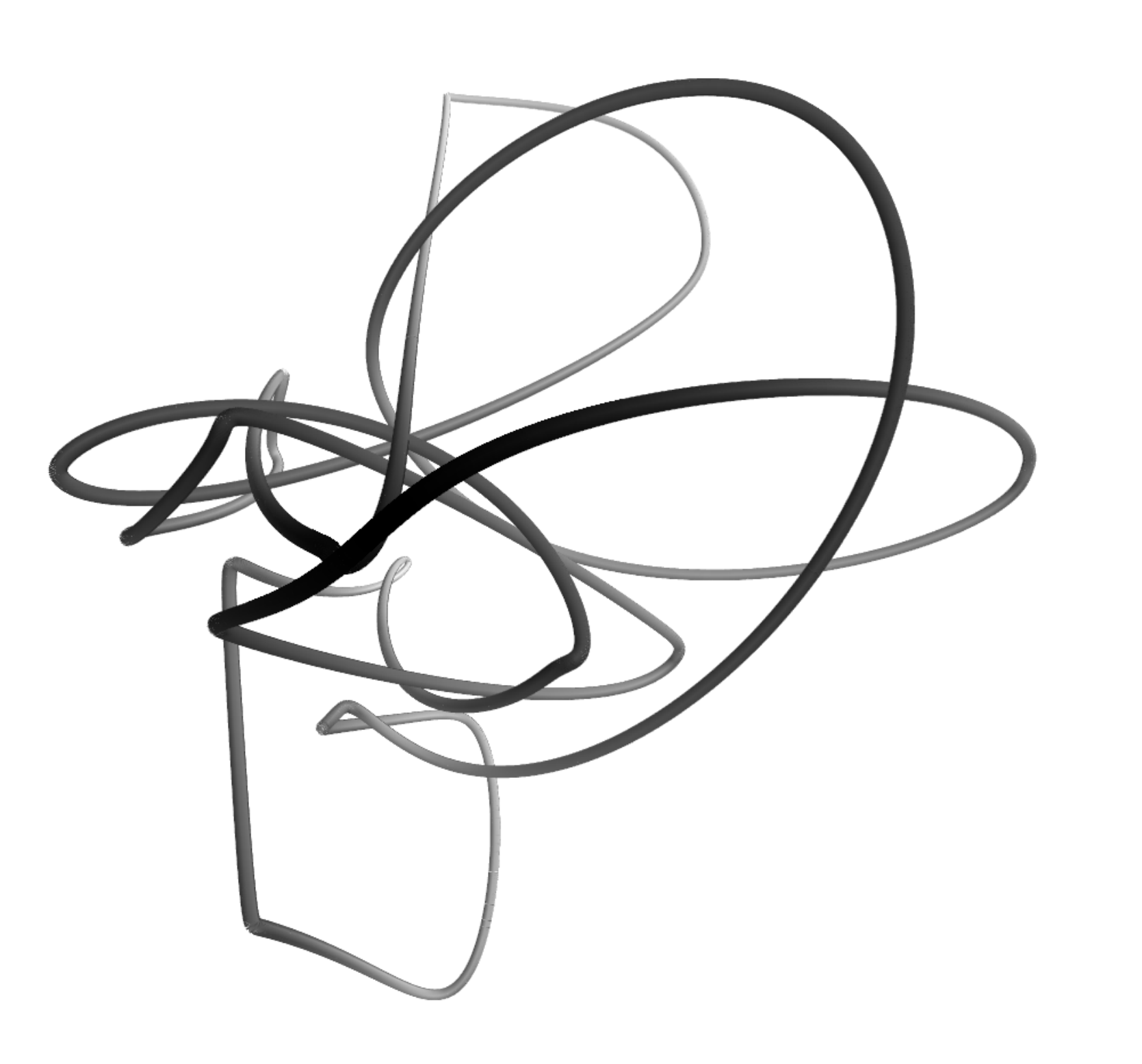
Most of our data is collected for loops of 10,000 segments and 10 harmonic modes; see Table 1. In Fig. 2 we show a sample initial loop. We evolve the loop as described in Sec. II and keep track of the fragmentations. We define loop “generations” in the following way. The initial loop is the first generation. When it splits into two loops, those are in the second generation, and so on for successive generations. Once a loop is in a stable configuration it is counted in each subsequent generation. For example, a stable loop that is generated in the third generation will be counted in the third, fourth, etc. generations. At every generation, we can plot the length distribution of loops as shown in Fig. 3. The plot shows that the second generation has roughly a uniform distribution of lengths but that the stable loop distribution is sharply peaked at small lengths. The stable loop length distributions are plotted in Fig. 4. Though very small loops are formed through fragmentation the peaks in this figure at show the resolution limit of the simulations. Clearly the bulk of the stable loops are above our resolution limit. For comparison the SP and CA results are shown and are in good agreement with our results.
From the length distribution we calculate the average length per generation for several values of . In Fig. 5 we show the average length scaled by for the stable loops. All the plots for asymptote to the same value, , which clearly demonstrates that the average length of stable loops is proportional to . The plot for asymptotes to and suggests that loops with only very low harmonics could behave differently from loops with high harmonics. However, even the value of is very close to and we will disregard this difference in the discussion below. Then the asymptote at implies that an initial loop with harmonics fragments into stable loops, as can also be read off from Table 1. Given that the initial loop is straight on the length scale , the stable loop is also composed of roughly straight segments of length . This result solidifies and quantifies the finding in Ref. [7] that fragmentation does not continue indefinitely to smaller and smaller loops.
In terms of the and curves on the KT sphere, since a loop with only the fundamental harmonic wraps around a great circle once, we expect that stable loops will wrap the sphere only a third of the way. Also, the discussion below shows that the and curves for the stable loops occur in two disconnected segments on the KT sphere. Hence each segment only covers a sixth of the KT sphere and can be thought of as an arc on the KT sphere that extends on average.
Our result that the stable loops are made from roughly straight segments can only work if the loops have kinks on them. It can be argued that the average number of kinks should be four [4]. Assume that there is an initial loop with pre-existing kinks. (In our numerical work, the initial loops were smooth and so .) Every intercommutation event adds four kinks and one extra loop to the system. Therefore after intercommutations there will be kinks and loops. So the average number of kinks per loop is which goes to in the large limit. The distribution of kinks, however, needs to be calculated numerically and is shown in Fig. 6. From this argument and the numerical simulations we have the picture that stable cosmic string loops have roughly straight sides and four corners (kinks) on average.
In general, stable loops have relativistic center of mass velocities as shown in Fig. 7. To analyze the shape of a stable loop, we must first transform to its center of mass frame. Care must be taken to transform the coordinates so that the gauge conditions in Eqs. (2) are satisfied as described in Appendix B. Let us denote the resulting curves on the KT-sphere in the rest frame by and .
To analyze the planarity of a stable loop, we calculate the “moment of inertia” tensors for and via
| (6) |
If the (and similarly for the ) curve is uniformly distributed on the KT-sphere, the three eigenvalues of the tensor would be equal. If one of the eigenvalues of vanishes, then is distributed in a plane; and if two eigenvalues vanish, the distribution is lineal. In Fig. 8 we show the average eigenvalues as the loop continues to fragment. It is clear that one of the eigenvalues vanishes, and the largest eigenvalue is much larger than the middle eigenvalue. So the curve is mostly in one direction on the KT-sphere (say around the -axis), with a little spread in some other direction. Since the centroid of the curve has to vanish in the center of mass frame (see the discussion below Eq. (3)), the curve must contain two short segments, say one near the north pole and the other near the south pole. In an idealized (“degenerate”) case, the curve would consist of just 2 points on the KT-sphere. Similarly the curve would consist of just 2 other points. Since the loop is a sum of the left- and right-movers, this implies that the loop is planar and defined by the plane of the and curves.
As another check of this picture, we have plotted the kink sharpness for the curves, defined as [8]
| (7) |
where are the values of on either side of the kink. The plot in Fig. 9 demonstrates a peak near sharpness of 1, which implies . This shows that there are 180 degree jumps on the KT-sphere, in accordance with our picture that the curve corresponds to two small anti-podal regions on the KT-sphere.
We can go a bit further and ask for correlations between the left- and right-movers. For this we plot the distribution of in Fig. 10. (Angular brackets denote average over a loop.) This plot shows that and tend to get more orthogonal with fragmentation.
This picture of stable loops implies that the and curves rarely cross each other and hence that cusps should be suppressed. For an initial loop with modes we expect it to contain approximately cusps. (Each mode roughly corresponds to a great circle on the KT-sphere so the number of intersections is proportional to .)
We have seen that on average stable loops are produced. If is the “cusp survival fraction” — the fraction of cusps on the initial loop that survive on the stable loops — then on average we expect cusps on each loop. Fig. 11 shows that, on average, each stable loop has a of containing a cusp independent of resolution and the number of modes on the initial loop so the cusp survival fraction is found to be . (We have verified this is true in our simulations but do not show the results here.)
IV Length dependent results
The focus of this work is on the average properties of all stable loops. The statistics we have presented give equal weights to all loops. For some observational signatures, however, long loops may be more relevant than small loops. Hence, in this section, we provide some statistics as a function of loop length. The results shown here are for the and runs. Logarithmic length bins are chosen based on the distribution of loop lengths (see Fig. 4). Ten bins are chosen between lengths of and . The initial bin begins at a length of to ensure that all loops are above our resolution limit; approximately of the loops are included. The final bin includes all loops with lengths longer than .
The results are shown in Figs. 12–15. These figures show the velocity, number of kinks, number of cusps, and eigenvalues, respectively, for each length bin. In the plots the error bar shows the width of the bin and the error bar provides the percentile range for the values. The results are as expected. The smallest loops are predominantly high velocity, contain approximately four kinks per loop, have a small chance of containing a cusp, and are planar. The largest loops are predominantly lower velocity, contain more than four kinks, have a higher chance of containing a cusp, and are less planar.
V Discussion
Our numerical results point to the picture that stable loops are deformations of degenerate kinky loops. In this section we provide further evidence for this picture by demonstrating that there exists a class of perturbed degenerate kinky loops that are stable.
We begin by describing the degenerate kinky loop [5],
| (8) |
where
| (9) |
denotes the greatest integer less than or equal to , and . In Fig. 16 we show some snapshots of a degenerate kinky loop.
Note that the degenerate kinky loop collapses to a double line twice during an oscillation period, yet the stable loops do not self-intersect. This must be due to the fact that stable loops are not exactly degenerate. To show that this is the case, consider
| (10) |
where and now
| (11) |
As illustrated in Fig. 17, these perturbations stretch out the point corresponding to on the KT-sphere for the degenerate kinky loop to an arc of length [5].
We can check explicitly that the self-intersection condition
| (12) |
is satisfied for such a loop if and only if (mod ), for any , that is, the loop does not intersect at any time. We first write the intersection condition in terms of and ,
| (13) |
Since for our loop (10) we have for all and , we also have , and self-intersection requires
| (14) |
The first condition is satisfied for or for . Only the latter possibility is of interest since we are looking for an intersection with . The second condition for the and components leads to
| (15) |
Note that both equations must be satisfied for a self-intersection to occur.
With the help of some trigonometric identities, we can rewrite (15) as
| (16) | |||||
Taking the ratio of these equations leads to
| (17) |
so that . By squaring and adding the equations, we obtain
| (18) |
so that the second relation in Eq. (16) leads to
| (19) |
or
| (20) |
which implies or else . (Solutions such as can be ignored because we restrict to lie in the interval and .) Therefore the only solution is of the type , or else , , which are both trivial. This shows that there are no self-intersections. The conclusion is intuitive since is obtained by integrating and hence is a vector that lies in the plane (see Fig. 17) and rotates in this plane. Since , never attains the same vector value twice for .
The perturbed degenerate kinky loop discussed above does not contain any cusps while our numerical results show that roughly half of the stable loops have a cusp. To understand the and curves of a stable loop with cusps we show an example of these curves for a sample loop from our numerical runs in Fig. 18 which contains three kinks and one cusp. In this example the curve is like our perturbed degenerate kinky loop but the curve is much more elongated. The two curves are in planes nearly perpendicular to each other.
To construct a stable loop with cusps consider
| (21) | |||||
where
| (22) |
and is an arbitrary phase. There are two cusps due to the intersections at . These occur at and . We have numerically confirmed that this loop is stable for the parameter choice
| (23) |
In Fig. 18 we show the and curves for a stable loop with cusps similar to (21) extracted from our simulations.

VI Conclusions
We have shown that the fragmentation of a large complicated loop yields stable quasi-planar, quasi-rectangular loops, that are similar to degenerate kinky loops. If cosmic string loops are the result of a large number of intercommutings – even as few as five or six intercommutings may be sufficient (e.g. Fig. 8) – we expect that they too will be quasi-rectangular. Earlier work has examined the stability of relatively simple loops (with a small number of harmonics) and found stability over a region of parameter space [9, 10, 11, 12]. It is unclear if cosmological evolution can directly produce these stable loops with few harmonics. Cosmological loops will certainly contain kinks and this feature is missing in the loops investigated in these earlier studies.
In a cosmological setting, when a loop is produced from the infinite string network, it will fragment down to stable loops within two oscillation periods, and therefore only stable loops are relevant for cosmological signatures. Indeed the aim of the CA and SQSP studies was to obtain the gravitational power emitted from realistic cosmic string loops. We can also estimate the gravitational power based on the analytical results of [5] for emission from degenerate, kinky loops, and obtain an estimate that is within 13% of the CA result. The gravitational power radiated from degenerate kinky loops is analytically calculated to be whereas CA numerically estimate from their simulations, where is the string tension.
For cosmic strings, Hubble expansion, frictional damping and radiation damping also come into play, though the effects are generally on very long time scales and depend on the environment in which the strings are placed. Hence we expect that when a large loop is produced from the network, it will fragment into stable loops within two oscillation periods and then, as these stable loops oscillate for many oscillation periods, damping effects start to play a role and to change the Nambu-Goto dynamics. So to characterize the effect of damping on the cosmic string network loops, we can limit our study to the damping effects on the perturbed degenerate kinky loops and the stable loops with cusps described above.
Acknowledgements.
We are grateful to Jose Blanco-Pillado, Ken Olum, Ben Shlaer and Alex Vilenkin for discussions and Isha Savani for help during the initial algorithm development. This work was supported by the U.S. Department of Energy at Case Western Reserve University. TV was also supported by grant number DE-FG02-90ER40542 at the Institute for Advanced Study. The numerical simulations were performed on the facilities provided by the Case ITS High Performance Computing Cluster.Appendix A Loop Intercommutation
The numerical evolution in this work was performed using the “diamond method” for string evolution which is discussed in [13]. Full details of our implementation along with source code and documentation is available online [6]. Here we will discuss one aspect of the evolution: loop intercommutation.
The diamond method gets its name from the grid shown in Fig. 19. The top of the figure shows the grid structure for an initial loop. Our initial loop segments are of uniform length, , producing a regular grid. This grid provides a simple geometric picture of the loop. With this grid structure, a starting point, , and values for and , taken to be piecewise constant functions, we can calculate the coordinate of the string during its evolution if intersections do not occur.
In Fig. 19 we consider the case of an intersection at points and , that is, . In this picture the intercommutation and production of two loops is geometric. The shaded area is excised from the parent loop to become one daughter loop (bottom right grid) and the remaining portions of the parent loop are reconnected (bottom left grid). The past light cone of the intersection point no longer contains meaningful information and has been removed from the new grids. When an intersection occurs the grid structure is modified; an originally uniform grid becomes non-uniform, but otherwise contains the same information. In the bottom left grid the light gray shaded diamonds are the remnants of the original diamonds that intersected. The dark gray shaded diamond is a new one created by the reconnection of the grid after the middle portion has been removed. These two grids now describe independent loops which may be evolved in the usual way for all times .
Appendix B Loop Rest Frame Transformation
The time coordinate of a loop, , was chosen to be the proper time and the same as the background spacetime, ; see Sec. II. To make and easier to boost we construct four-vectors from them with the time components give by and . At a fixed time, , we may then write in the initial loop’s rest frame
| (24) |
where .
The center of mass velocity of a loop is given by
| (25) | |||||
With boosting to the rest frame of this loop we find
| (26) |
Notice that the time component of this four-vector is no longer . To correct this we apply a gauge transformation to the coordinate . Let
| (27) |
so that
| (28) |
An integration gives and a coordinate rescaling can be used to bring the interval back to . With this we now have
| (29) | |||||
where we have used (26) for . Applying the same transformation to the spatial piece of (26) we find
| (30) |
Again this looks messy but we can verify that , as required. We can further verify that
| (31) |
For we proceed in the same way. In this case the gauge transformation is and we find
| (32) |
Once again we can show that .
The above equations are not in the best form for numerical evaluation. If then so large number will be subtracted from each other in the numerator. To correct this it is better to write the equations in terms of since . This provides the alternative forms
| (33) |
Appendix C Explicit Solutions of the String Equations and Constraints
Here we describe an explicit analytical solution of the Nambu-Goto equations of motion, Eq. (1), and the string constraints, Eqs. (2), (3). By choosing the decomposition in terms of left- and right- movers we can solve the Nambu-Goto equations as in Eq. (1). To solve the constraint in Eq. (2) we start with
| (34) |
where and are functions of . We similarly choose with independent angular functions.
We require that be periodic under . (Throughout this section we consider a loop of length .) Therefore we write
| (35) |
where is an integer, and and are arbitrary constants that can be chosen randomly to generate random loops. Similarly,
| (36) |
where is an integer, and and are arbitrary constants.
Next we come to the closure condition in Eq. (3). The integral of will, in general, not vanish. To correct this, define
| (37) |
and boost to velocity followed by a gauge transformation as described in Appendix B. This gives us the final solution,
| (38) |
where and
| (39) |
As in Appendix B, an integration shows that and a coordinate rescaling can be used to bring the interval back to .
It is straightforward to check directly that and also
| (40) |
In a similar way we construct .
This scheme has the advantage that it solves the constraints exactly and explicitly though it still requires integrating to find and . We have not employed this scheme in the work reported here but have remained with the SP algorithm to facilitate comparison.
References
- [1] A. Vilenkin and E. P. S. Shellard, Cosmic strings and other topological defects, Cambridge monographs on mathematical physics (Cambridge Univ. Press, Cambridge, 1994).
- [2] R. J. Scherrer and W. H. Press, Phys. Rev. D 39, 371 (1989).
- [3] R. J. Scherrer, J. M. Quashnock, D. N. Spergel, and W. H. Press, Phys. Rev. D 42, 1908 (1990).
- [4] P. Casper and B. Allen, Phys. Rev. D 52, 4337 (1995), arXiv:gr-qc/9505018 .
- [5] D. Garfinkle and T. Vachaspati, Phys. Rev. D 36, 2229 (1987).
- [6] C. J. Copi, “Cosmic String Information,” http://www.phys.cwru.edu/projects/strings/ (2010), source code and documentation is available.
- [7] D. P. Bennett and F. R. Bouchet, Phys. Rev. Lett. 60, 257 (1988).
- [8] E. J. Copeland and T. W. B. Kibble, Phys. Rev. D 80, 123523 (2009), arXiv:0909.1960 [astro-ph.CO] .
- [9] E. J. Copeland and N. Turok, Physics Letters B 173, 129 (1986).
- [10] A. L. Chen, D. A. DiCarlo, and S. A. Hotes, Phys. Rev. D 37, 863 (1988).
- [11] D. DeLaney, K. Engle, and X. Scheick, Phys. Rev. D 41, 1775 (1990).
- [12] X. A. Siemens and T. W. B. Kibble, Nuclear Physics B 438, 307 (1995), arXiv:hep-ph/9412216 .
- [13] V. Vanchurin, K. Olum, and A. Vilenkin, Phys. Rev. D 72, 063514 (2005), arXiv:gr-qc/0501040 .