Implications of Dramatic Broad Absorption Line Variability in the Quasar FBQS J1408+3054
Abstract
We have observed a dramatic change in the spectrum of the formerly heavily absorbed ‘overlapping-trough’ iron low-ionization broad absorption line (FeLoBAL) quasar FBQS J1408+3054. Over a time span of between 0.6 to 5 rest-frame years, the Mg ii trough outflowing at 12,000 km s-1 decreased in equivalent width by a factor of two and the Fe ii troughs at the same velocity disappeared. The most likely explanation for the variability is that a structure in the BAL outflow moved out of our line of sight to the ultraviolet continuum emitting region of the quasar’s accretion disk. Given the size of that region, this structure must have a transverse velocity of between 2600 km s-1 and 22,000 km s-1. In the context of a simple outflow model, we show that this BAL structure is located between approximately 5800 and 46,000 Schwarzschild radii from the black hole. That distance corresponds to 1.7 to 14 pc, 11 to 88 times farther from the black hole than the H broad-line region. The high velocities and the parsec-scale distance for at least this one FeLoBAL outflow mean that not all FeLoBAL outflows can be associated with galaxy-scale outflows in ultraluminous infrared galaxies transitioning to unobscured quasars. The change of FBQS J1408+3054 from an FeLoBAL to a LoBAL quasar also means that if (some) FeLoBAL quasars have multiwavelength properties which distinguish them from HiBAL quasars, then some LoBAL quasars will share those properties. Finally, we extend previous work on how multiple-epoch spectroscopy of BAL and non-BAL quasars can be used to constrain the average lifetime of BAL episodes (currently 60 rest-frame years at 90% confidence).
Keywords:
galaxies: active – quasars: general – quasars: absorption lines – quasars: individual: FBQS J1408+3054.1 Introduction
Broad Absorption Line (BAL) quasars are a subset of quasars which exhibit strong absorption troughs from gas flowing outwards with velocities of thousands to tens of thousands of km s-1 (e.g., Allen et al. 2010). The traditional definition is that BAL quasars are those which have C iv absorption which dips at least 10% below the continuum level for a contiguous stretch of at least 2000 km s-1 at blueshifts of 3000 km s-1 relative to the quasar (Weymann et al. 1991). Other proposed definitions (Hall et al. 2002; Trump et al. 2006; Gibson et al. 2009) relax some of the conditions of the traditional definition to include more cases of potential intrinsic absorption with the tradeoff of increased contamination by blended narrow absorbers (Knigge et al. 2008) whose origin(s), especially at low outflow velocities, may differ from those of BAL outflows.
BAL quasars are often classified into three subtypes: high-ionization (HiBAL), low-ionization (LoBAL) and iron LoBAL (FeLoBAL). HiBAL quasars show absorption from only relatively high-ionization species such as C iv and N v. LoBAL quasars show high-ionization features plus absorption from low-ionization species such as Mg ii and Al iii. ‘Iron LoBAL’ (Becker et al. 1997) or ‘FeLoBAL’ (Becker et al. 2000) quasars show high- and low-ionization troughs plus absorption from excited states of Fe ii, Fe iii, or both. There is no commonly accepted definition for how broad or deep the Mg ii or Fe ii absorption has to be for a quasar to be classified as a LoBAL or FeLoBAL quasar (Trump et al. 2006; Gibson et al. 2009; Zhang et al. 2010). However, such troughs should at least be broader than intervening Mg ii absorption systems, the vast majority of which have widths 500 km s-1 (Mshar et al. 2007). A minimum depth of 10% is appropriate for LoBAL and FeLoBAL troughs just as for HiBAL troughs, though in all cases this is not a physical limit but reflects the limitations imposed by spectral signal-to-noise ratios and our inability to model quasar continua exactly.
BAL troughs are often highly saturated, so that the trough depth is determined less by the gas column density and more by the covering fraction; that is, the fraction of the continuum source occulted by the absorbing structure (e.g., Arav et al. 1999). Variability in BAL trough strengths is relatively common (see the exhaustive reference list in Hall et al. 2007, and Gibson et al. 2008) but large (50%) changes in absorption equivalent width are rare (Crenshaw et al. 2000; Lundgren et al. 2007; Hamann et al. 2009; Leighly et al. 2009; Gibson et al. 2010).
The =0.848 quasar FBQS J140806.2+305448 (hereafter FBQS J1408+3054) was first reported by Gregg et al. (1996), where it was misclassified as a star, and was first identified as a LoBAL quasar in White et al. (2000). Hall et al. (2002) described it as a member of the class of ‘overlapping-trough’ FeLoBAL quasars because its Fe ii absorption troughs are broad enough to overlap and yield almost no continuum windows below 2800 Å. However, the covering fraction of its Fe ii absorption was only 75% at its discovery epoch, unlike some overlapping-trough objects which have 95% covering fractions. FBQS J1408+3054 also likely has an FR II radio morphology (Gregg et al. 2006).
In this work we present spectroscopy of FBQS J1408+3054 spanning nearly 8 years in its rest frame. The spectroscopic dataset shows mild variability followed by a dramatic decline in Fe ii and Mg ii absorption strength (§ 2). Substantial trough variability has previously been observed in the overlapping-trough FeLoBAL quasar SDSS J043742.81004517.6 (Hall et al. 2002), but FBQS J1408+3054 is the first known case of an FeLoBAL spectrum changing to a LoBAL spectrum.11 1 We note that the absorption system D+E in NGC 4151, while too narrow (FWHM = 435 km s-1) and low-velocity (491 km s-1) to qualify as a BAL trough, exhibited only Mg ii absorption in 1994-1996 but also exhibited strong Fe ii absorption in 1999 (Kraemer et al. 2001) and weak Fe ii absorption in 2002 (Kraemer et al. 2006), indicative of transverse motion of an intrinsic quasar absorption system such as that reported herein. We estimate a black hole mass for FBQS J1408+3054 in § 3. In § 4 we constrain the BAL structure’s size and transverse velocity and present a simple outflow model which we use to constrain the BAL structure’s location and age. We also discuss the implications of our observations for the average episodic lifetime of BAL troughs in quasar spectra and for the link(s) between BAL subtypes and between BAL troughs and FR II radio morphologies. We end with our conclusions in § 5.
2 Data
2.1 Optical Spectroscopy
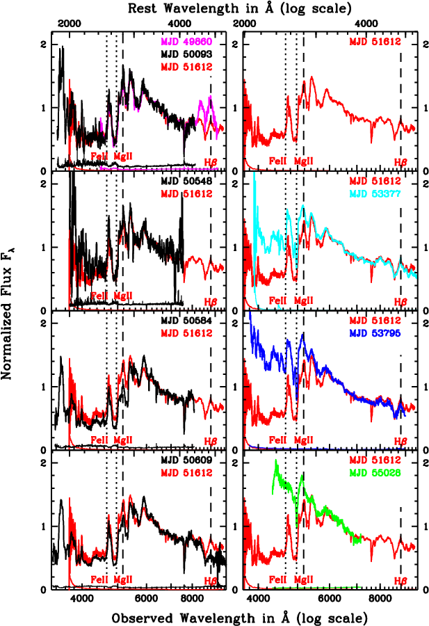

Spectroscopy was obtained using numerous telescope and instrument combinations (Table 1), including the Echellette Spectrograph and Imager (ESI; Sheinis et al. 2002) at the Keck telescope, the Kast Spectrograph on the Lick Observatory 3m Shane telescope (Miller & Stone 1993), and the Low Resolution Spectrograph (LRS; Hill et al. 1998) on the Hobby-Eberly Telescope (HET). Data were obtained, reduced and calibrated using standard procedures (Gregg et al. 1996; White et al. 2000; Gregg et al. 2002), except as we now discuss with regard to the HET spectrum.
We obtained a spectrum of FBQS J1408+3054 with the LRS on the HET with the g2 grism (useful observed wavelength coverage 4335-7155 Å) and a 1 slit. We obtained two spectrograms with a total exposure of 1510 seconds in 2 seeing at an average airmass of 1.26. A flux calibration star was not observed. We used the known throughput of the instrumental configuration to remove the instrumental response before correcting for interstellar and atmospheric extinction. When compared to the other normalized spectra shown in Figure 1, the normalized HET spectrum exhibited a large-scale curvature resulting in a downturn in flux over several hundred observed Å at both ends of the spectrum. We believe this curvature resulted from slit losses due to differential refraction. For the slit to include the quasar and a star bright enough to guide on, the long axis of the slit had to be oriented about 82∘ from the parallactic angle, resulting in differential refraction of 0.75 over our wavelength range (Table I of Filippenko 1982, hereafter F82). Inspection of the results of the two individual exposures obtained showed that one exposure yielded a more prominent downturn in its spectrum and also showed more flux from a third object slightly offset from the centre of the slit, suggesting that the quasar was not well centred in the slit in that exposure. We therefore dropped that exposure from consideration. To correct for slit losses in the remaining exposure, we assumed that the target was centred in the slit at a wavelength of 6500 Å. We computed the offset of the target along the narrow axis of the slit from 4000-7500 Å using Table I of F82. We then used equation 8 of F82 to calculate the fraction of the flux captured by the slit as a function of wavelength and corrected the spectrum for those wavelength-dependent losses.
The panels of Figure 1 show all of our spectra of FBQS J1408+3054 taken between 1995 and 2009, normalized to an average of unity between observed 6000 Å and 7000 Å. The dashed vertical lines show the wavelengths of H and Mg ii emission in the quasar rest frame. The dotted vertical lines show absorption from Fe ii 2632 and Mg ii 2796,2803 at the redshift of maximum absorption (=0.775, a blueshift of 12,000 km s-1 from the quasar rest frame). Blueward of Fe ii 2632, the spectra suffer overlapping absorption from hundreds of transitions of Fe ii. A strong decrease in absorption strength occurred over the 955 rest-frame days between the two Keck epochs (MJDs 51612, in red, and 53377, in cyan). The absorption was still dramatically weaker in the Sloan Digital Sky Survey (SDSS; York et al. 2000) spectrum (in blue) taken on MJD 53795, 123 rest-frame days after the second Keck epoch, and made available in the SDSS Seventh Data Release (DR7; Abazajian et al. 2009). The corrected HET spectrum, taken 668 rest-frame days after the SDSS epoch and shown in green in the lower right panel of Figure 1, reveals Mg ii absorption even weaker than in the SDSS epoch and a complete lack of Fe ii UV1 absorption.
Figure 2 displays our near-ultraviolet spectra of FBQS J1408+3054 from the period of weakening absorption. Wavelengths (in Å) are given in the rest frame of peak absorption (=0.775) along the bottom and in the quasar rest frame (=0.848) along the top. As in Figure 1, the vertical dashed line shows the wavelength of Mg ii in the quasar rest frame defined by the H line (in the more recent spectra, the Mg ii peak is blueshifted relative to the H rest frame) and the rightmost vertical dotted line shows the wavelength of Mg ii at the velocity of peak absorption, while the leftmost dotted line shows absorption at the same velocity from Fe ii 2632, the longest-wavelength component of the Fe ii UV1 multiplet (Moore 1950). The left two light grey shaded regions show the wavelength ranges absorbed by Fe ii multiplets UV2+UV3 and UV1 at =0.775; as expected, Fe ii 2632 traces the long-wavelength edge of the UV1 absorption trough. Absorption outside the shaded regions arises predominantly from hundreds of excited Fe ii transitions whose troughs overlap in velocity space.
The dark grey shaded region shows the wavelength range spanned by Mg ii absorption at velocities =8700 km s-1 to =14,200 km s-1. The rightmost light grey shaded region shows the wavelength ranges absorbed by a blend of Fe ii UV62 + higher-velocity Mg ii absorption. This high-velocity wing of the Mg ii trough extends to 2623 Å in the quasar rest frame (=19,500 km s-1), as seen in the HET spectrum from MJD 55028 (green). The absorption at those wavelengths in the HET spectrum cannot be Fe ii UV62 because the Fe ii UV62 multiplet is intrinsically weaker than the UV1 multiplet and the latter is not present in the HET spectrum. Without detailed modeling, it is impossible to be sure that the Fe ii absorption spanned the same velocity range as Mg ii, but the shape of the MJD 51612 spectrum is consistent with Fe ii UV62 absorption also extending to 19,500 km s-1.
Figure 3 shows the Mg ii and blended Mg ii+Fe ii UV62 rest-frame equivalent widths for all spectra in Figure 1. The equivalent widths were measured relative to a continuum established using the normalized SDSS spectrum shown in Figure 1. In that spectrum, a linear continuum in vs. was drawn between the average fluxes at rest-frame 2550-2600 Å and 3765-3820 Å. In all spectra, Mg ii values were measured between 2670-2720 Å and Mg ii+Fe ii UV62 values were measured between 2585-2720 Å. While there is some uncertainty in the actual continuum level and thus in the measured , the changes in in Figure 3 are much larger than those uncertainties. As the Mg ii+Fe ii UV62 blend consists only of high-velocity Mg ii in the HET epoch, we conservatively estimate that the of Mg ii had decreased by a factor of two by the HET epoch.

2.2 Multiwavelength Photometry
In Table 2, we present time-ordered observed and synthesized photometric magnitudes and colours of FBQS J1408+3054. The photographic magnitudes listed are the average of the USNO-B1.0 (Monet et al. 2003) and GSC2.3.2 (Lasker et al. 2008) magnitudes whenever available and are typically uncertain by 0.4 (as compared to 0.02 for SDSS magnitudes). The conversions to SDSS magnitudes were made using equation 2 of Monet et al. (2003) except for the Palomar Quick which used Table 7 of Smith et al. (2002). In five spectroscopic epochs, the wavelength coverage was sufficient to enable synthesis of and colours using the SDSS system response curves of Doi et al. (2010) but slit losses prevented the synthesis of accurate magnitudes. Only in the SDSS spectroscopic epoch could both colours and magnitudes be reliably synthesized. Corrections for Galactic extinction have not been applied to these magnitudes.
Despite the uncertainties in the magnitudes in Table 2, the colours obtained from them provide good evidence that the -band absorption in FBQS J1408+3054 was approximately constant in strength for at least 27 rest-frame years prior to its weakening sometime after MJD 51612. However, we cannot rule out the disappearance and reappearance of an Fe ii BAL structure during that time, especially because there is a gap in the historical photometric record longer than twice the timescale over which the Fe ii absorption was later observed to vanish.
In the two SDSS photometric epochs, there was an 18% increase in -band flux relative to the -band flux between MJD 53110 and 53795 (371 rest-frame days). Assuming that flux increase was uniform across the band, we can predict that at MJD 53110 (rest-frame day 1759) the Mg ii+Fe ii trough had Å and the Mg ii trough Å. These points are plotted in Figure 3 without error bars. They suggest that the change in values during the weakening of the BAL troughs may have been more gradual than rapid, and perhaps not monotonic.
To add to our picture of FBQS J1408+3054, we also searched for additional data at other wavelengths (Figure 4). We checked for sensitive X-ray coverage, but none is available. FBQS J1408+3054 was detected by 2MASS [Skrutskie et al. 2006] in 1999 (MJD 51517). With GALEX [Morrissey et al. 2007], FBQS J1408+3054 was detected in the NUV filter in 2005 (MJD 53523.5) and in both the NUV and FUV filters in 2007 (MJD 54224.5). The flux decrement between the NUV and FUV filters is consistent with the expected strong absorption in the Lyman transitions at the quasar redshift. The FUV non-detection on MJD 53523.5 is consistent with the fainter NUV flux at the same epoch. Both GALEX observations occurred after the MJD 53377 Keck spectrum which shows a strong reduction in Fe ii and Mg ii absorption strength, so we cannot determine if the absorption at observed NUV wavelengths has weakened like that at observed optical wavelengths has. The MJD 53523.5 NUV flux level is consistent with the MJD 53377 Keck spectrum, and the MJD 54224.5 NUV flux level is consistent with a continued decrease in absorption.
| Date | MJD | Source | 22 2 Rest-frame days since the first spectroscopic epoch. | 33 3 Rest-frame days since the previous spectroscopic epoch. | |
|---|---|---|---|---|---|
| 1995-05-23 | 49860 | KPNO 4m | 1000 | 0 | … |
| 1996-01-11 | 50093 | Lick Kast | 835 | 126 | 126 |
| 1997-04-10 | 50548 | KPNO 2.1m | 1250 | 372 | 246 |
| 1997-05-16 | 50584 | Lick Kast | 835 | 392 | 20 |
| 1997-06-10 | 50609 | Lick Kast | 835 | 405 | 13 |
| 2000-03-09 | 51612 | Keck ESI | 6750 | 948 | 543 |
| 2005-01-07 | 53377 | Keck ESI | 6750 | 1903 | 955 |
| 2006-03-01 | 53795 | SDSS DR7 | 1850 | 2129 | 226 |
| 2009-07-16 | 55028 | HET LRS | 1130 | 2797 | 668 |
| Date | MJD | Source | Original | g | r | i | gr | ri |
|---|---|---|---|---|---|---|---|---|
| 1950-04-18 | 33389 | POSS-I | O=19.2 | 18.6 | … | … | … | … |
| 1950-04-18 | 33389 | POSS-I | E=17.1 | … | 17.4 | … | 1.2 | … |
| 1982-05-21 | 45110 | Palomar | V=17.5 | 18.3 | … | … | … | … |
| 1992-04-08 | 48720 | POSS-II | J=19.0 | 18.8 | … | … | … | … |
| 1992-04-26 | 48738 | POSS-II | F=17.3 | … | 17.4 | … | 1.4 | … |
| 1995-02-23 | 49771 | POSS-II | N=17.0 | … | … | 17.4 | … | … |
| 1996-01-11 | 50093 | Licka | … | … | … | … | 0.95 | 0.05 |
| 1997-04-10 | 50548 | Licka | … | … | … | … | 0.78 | … |
| 1997-05-16 | 50584 | Licka | … | … | … | … | 1.28 | 0.01 |
| 1997-06-10 | 50609 | Licka | … | … | … | … | 1.15 | 0.05 |
| 1999-12-05 | 51517 | 2MASS | … | … | … | … | … | … |
| 2000-03-09 | 51612 | Kecka | … | … | … | … | 0.95 | 0.09 |
| 2004-04-13 | 53108 | SDSS | g,r,i | 17.82 | 17.40 | 17.33 | 0.42 | 0.07 |
| 2004-04-15 | 53110 | SDSS | g,r,i | 17.84 | 17.40 | 17.34 | 0.44 | 0.06 |
| 2005-01-07 | 53377 | Kecka | … | … | … | … | 0.48 | 0.07 |
| 2005-06-02 | 53524 | GALEX | … | … | … | … | … | … |
| 2006-03-01 | 53795 | SDSS44 4 Synthesized from spectroscopy; see text. | … | 17.76 | 17.47 | 17.44 | 0.29 | 0.03 |
| 2007-05-04 | 54225 | GALEX | … | … | … | … | … | … |

3 Black Hole Mass Estimate
To estimate the black hole mass of this quasar using the FWHM (Full Width at Half Maximum) of its H emission line, we must remove the neighboring Fe ii emission.
We subtracted Fe ii emission from the MJD 53377 Keck ESI spectrum using two templates: Boroson & Green (1992; BG92) and Véron-Cetty et al. (2004; VJV04), both convolved with Gaussians of FWHM spaced every 250 km s-1 from 1000 to 20,750 km s-1. First, we subtracted a power-law continuum fit made using observed-frame windows 7007-7079 Å and 10280-10351 Å (rest-frame 3791-3830 Å and 5562-5601 Å).55 5 This fit lies above the observed spectrum around 4685 Å, suggesting that FBQS J1408+3054 is one of the rare class of Balmer-line BAL quasars (Wang et al. 2008, and references therein). Fe ii subtraction confirms that a significant H trough exists. The trough is blueshifted by 11,000 km s-1, so it does not significantly affect the measurement of the H FWHM. Although the H BAL appears to be deeper on MJD 51612 than on MJD 53377, we cannot reliably claim a detection of variability. The relative flux calibration uncertainties are larger this close to the long-wavelength end of the spectrum, and apparent variability in the Fe ii emission could affect the appearance of the H trough, but no H continuum fit or Fe ii subtraction is possible for the MJD 51612 spectrum due to its limited wavelength coverage longward of H. Next, each velocity-broadened Fe ii template was scaled using a progressively increasing normalization factor and the value between the spectrum and each normalized template was measured using the rest-frame region 4440-4647 Å. The normalization factor with the lowest for any velocity FWHM was chosen; the best-fit Fe ii FWHM was 3000 km s-1 in both cases.
The resulting Fe ii-subtracted spectra were used to measure the H FWHM. After subtraction of the VJV04 template, we obtained FWHM=4100 km s-1. After subtraction of the BG92 template, we obtained FWHM=3800 km s-1.
To determine the black hole mass from H, we use the formula from Onken et al. (2004), where is the gravitational constant. To determine we use the formula in Bentz et al. (2009):
| (1) |
where the H broad-line region radius is in light-days, Å rest-frame and is the monochromatic luminosity there. We measure ergs s-1 cm-2 Å-1, which corresponds to ergs s-1 in a Universe with km s-1 Mpc-1, and . These quantities yield light-days (0.16 parsecs) or km.
We thus find using the VJV04 template and using the BG92 template. We adopt , which yields a Schwarzschild radius of km, so that . Using the mean bolometric correction of Richards et al. (2006), we estimate an unremarkable for this object.
4 Discussion
The trough variations in FBQS J1408+3054 are likely due to motions of absorbing gas transverse to our line of sight (e.g., Hamann et al. 2009). Such motions are seen in numerical simulations of line-driven outflows, both two-dimensional (Proga, Stone & Kallman 2000; Proga & Kallman 2004) and three-dimensional (Kurosawa & Proga 2009). In this section we first discuss why a changing ionization explanation for the trough variations is unlikely. Then we combine an estimate of the ultraviolet (UV) continuum source size in this object with the timescale over which the absorption disappears to estimate the transverse velocity of the absorbing gas. We then outline a simple BAL outflow model with which we constrain the distance of the absorbing gas from the black hole and the time since the gas was launched as part of the outflow. We close by discussing the implications of our results for the connections between BAL subtypes, for the average episodic lifetimes of BAL outflows and for the link between FR II radio morphology and BAL quasars.
4.1 Was the Fe ii Ionized Away?
One reason it is unlikely that the changes in the BAL troughs of FBQS J1408+3054 are due to a increased ionization of the absorbing gas is because the near-UV continuum flux of this quasar did not increase significantly while the absorption troughs weakened dramatically. The 1997 spectrum presented in Becker et al. (2000) and the 2006 SDSS spectrum show the same peak flux density near Mg ii to within 10%, and SDSS photometry of FBQS J1408+3054 taken on MJD 53110 yields magnitudes within 10% of magnitudes synthesized from SDSS spectroscopy taken on MJD 53795.
Of course, ionization is caused not by near-ultraviolet photons but by extreme UV and soft X-ray photons with Å, and along BAL quasar sightlines such photons are thought to be absorbed by a layer of shielding gas (e.g., Gallagher et al. 2006). It is possible that a decrease in the amount of shielding gas along our line of sight could have increased the ionizing flux without increasing the near-UV flux that we have observed, resulting in the ionization of the Fe ii absorber to Fe iii. Increasing ionizing flux would have expanded the Fe ii ionization front along our line of sight outwards. The timescale for that expansion is the timescale for the decrease in the shielding gas column or the recombination timescale in the Fe ii absorber, whichever is longer. The recombination timescale is , where =1.0210-12 cm-3 s-1 is the total recombination coefficient of Fe ii at =104 K (Woods et al. 1981) and is the Fe ii absorber’s electron density.
We cannot definitively rule out a change in ionizing flux as the explanation for the disappearance of Fe ii absorption in FBQS J1408+3054 because we lack X-ray data bracketing the disappearance epoch. We do not believe such an explanation is likely, however, because no evidence for ionization-dependent absorption variations has been found for the general population of BAL quasars (Gibson et al. 2008). Nonetheless, if a decreasing shielding gas column was responsible for Fe ii vanishing from the spectrum of FBQS J1408+3054, we can set a lower limit on in the Fe ii absorber of between cm-3 and cm-3 corresponding to the decrease occurring on the maximum or minimum observed timescales, respectively.
4.2 Constraints on the BAL Structure Size and Transverse Velocity
We refer to the gas that absorbs the quasar’s light in Mg ii and Fe ii as the BAL structure. Our conclusions about its size and location hold regardless of whether the structure is a single large cloud, part of a continuous flow tube (e.g., Arav et al. 1999), or a collection of smaller subunits (e.g., Hall et al. 2007). The column density of the absorption may vary over the structure even in the first two cases above (de Kool et al. 2002; Arav et al. 2005; Sabra & Hamann 2005), but for convenience we assume the structure has a sharp edge. Note that the entire BAL outflow can be much larger in size than the BAL structure we observe along our sightline (including extending to greater distances from the quasar) and can have a longer lifetime as well.
Given the size of the continuum source, the timescale over which absorption changes from strong to weak (or vice versa) constrains the velocity and location of the BAL structure. Furthermore, the length of time the quasar was seen as a BAL quasar constrains the size of the BAL structure in one transverse direction. For our discussion, we take the change in the spectrum of FBQS J1408+3054 that began between 2000 and 2005 to be a change from strong to weak absorption.
The minimum timescale over which the Fe ii troughs disappeared is the time between the 2005 and 2006 spectra: =226 rest-frame days. The maximum allowed timescale is the time between the 2000 and 2009 spectra: =1849 rest-frame days. We adopt an intermediate timescale of rest-frame days as the time required for the Mg ii+Fe ii rest-frame equivalent width to decrease from its level in 2000 to its level in 2009 at the rate of change observed between 2005 and 2006.
This value of rest-frame days is an estimate of the crossing time of the quasar emission region by the trailing edge of the BAL structure.66 6 We have assumed a sharp-edged structure, but the results apply generally. Because the Fe ii absorption goes from its maximum to zero in 946 rest-frame days, a diffuse structure in which gradually changes at the edges would have to move across the face of FBQS J1408+3054 faster than a sharp-edged structure. Therefore, the minimum transverse velocity derived for a sharp-edged structure is a lower limit to the velocity of any structure. As the quasar was seen as an FeLoBAL quasar of roughly constant for at least 948 rest-frame days prior to the 2000 epoch, the time required for the entire BAL structure observed in FBQS J1408+3054 since its discovery to cross the quasar emission region was at least . In other words, the entire BAL structure took at least twice as long to cross the quasar emission line region as the edge of the BAL structure did.77 7 The lack of strong variability in the historical photometry of FBQS J1408+3054 discussed in § 2.2 suggests that the BAL structure actually had a crossing time of 27 rest-frame years, 10 times longer than the crossing time of its edge. However, as we lack spectroscopy or regularly sampled photometry in pre-discovery epochs, we quote the shorter timescale to be conservative. Twice the 2700 Å continuum emission region size is thus an approximate lower limit on the transverse size of the BAL structure in the direction of its projected motion on the sky. The maximum depth of the Fe ii absorption reveals that the BAL structure covered at least 75% of the region that produces the continuum emission at 2700 Å (and possibly part of the Fe ii-emitting region, but not all; see below). Because this covering fraction was roughly constant for several rest-frame years, we take it to be the extent of the BAL structure in the direction on the sky orthogonal to the structure’s motion on the sky.
We use a Shakura & Sunyaev (1973) thin accretion disk model to estimate , the diameter of the disk within which 90% of the 2700 Å continuum is emitted, for a black hole. We find km (46). The projected dimensions of the BAL structure are therefore km or 0.01 pc wisde by km or 0.028 pc (and likely km or 0.28 pc) long in its projected direction of motion.
Using and , we can constrain the velocity of the BAL structure perpendicular to our line of sight: km s-1, where the range comes from the constraints on . The uncertainty on the size of the region crossed by the flow can change these limits somewhat (see the end of the next section). Nonetheless, the transverse velocity is constrained to be approximately 2600 km s-1 22,000 km s-1); for comparison, the line-of-sight velocity of peak absorption is a blueshift of 12,000 km s-1.
We can rule out the possibility that the BAL structure completely crossed the larger Fe ii-emitting region during the time span . If we use instead of as the size of the region crossed by the BAL structure, will increase. As the Fe ii FWHM in this object is smaller than the H FWHM, Fe ii emission is likely to come from a larger average radius than H. Assuming , we obtain km = 910. In that case, we find km s-1. Such a high velocity implies a small distance from the quasar, which is not self-consistent. A BAL structure located at any distance would not be able to cover the full extent of the Fe ii emission region.
4.3 A Model for Constraining the BAL Structure Location
When the radial velocity of absorbing gas around a quasar is not known, its distance from the black hole is usually estimated by assuming it is in a circular orbit (e.g., Risaliti et al. 2007). However, in our case the radial velocity of the BAL gas is 12,000 km s-1 and we cannot self-consistently assume a circular orbit. To estimate the distance of the BAL structure from the black hole, , some assumptions about the velocity field of the BAL wind must be made (see, e.g., § 6.2 of Misawa et al. 2005).
Given the large blueshift of the BAL structure in FBQS J1408+3054, the outflow was likely launched at a radius where the escape velocity is comparable to the observed blueshift (e.g., Murray et al. 1995; Proga, Stone & Drew 1998; Proga 1999; Everett 2005; Zhang & Thompson 2010). A natural source for such gas is a wind from the accretion disk around the quasar, and that is the scenario we adopt.
We assume that our line of sight to the quasar lies at a latitude above the accretion disk and that the accretion disk has azimuthal symmetry (Figure 5). The BAL wind crosses our line of sight to the continuum emission region at a distance from the black hole, at cylindrical coordinates and . We parametrize the velocity field of the BAL wind at this point as an azimuthal velocity and a poloidal velocity oriented at an angle above the accretion disk.88 8 The magnitude of the three-dimensional velocity of the BAL wind at this point is given by . The BAL velocity components parallel and perpendicular to our line of sight are
| (2) |
| (3) |
We know from spectroscopy, and the BAL variability constrains .


To link these velocities to , we first assume that the BAL outflow started out in a circular orbit at radius in the accretion disk and has not swept up a significant amount of mass since then. We assume conservation of angular momentum in the direction (neglecting momentum carried by magnetic fields) so:
| (4) |
where is the current distance of the BAL structure from the axis of symmetry of the accretion disk.
Next, we use the results of Murray et al. (1995, fig. 3) and Murray & Chiang (1998, equation 2) that the final poloidal velocity of a radiatively driven outflow launched from radius is and that is reached within a radial distance of a few times . Therefore, we assume
| (5) |
and write
| (6) |
| (7) |
These equations express and in terms of physical parameters in our outflow model, in principle enabling us to constrain those parameters and place limits on .
In the case of known and , can be obtained from equation 6. A lower limit on then yields an upper limit on via equation 7, and an upper limit on follows. Similarly, a lower limit on follows from an upper limit on .
Note that if , the streamlines must have bent to reach the location with velocity at angle . The streamlines therefore must also have crossed our line of sight at another position closer to the black hole (Figure 5, right-hand panel), possibly producing another BAL trough in the spectrum. Another trough is guaranteed to be produced only if the BAL outflow is continuous back to the launch radius and extends over all azimuthal angles.
We make one final refinement to the above analysis. We have assumed that continuum emission region is intrinsically circular with diameter , projected on the sky to an ellipse of major axis . The transverse velocity limits were computed assuming a distance was crossed by the BAL flow, but in fact the trailing edge of the BAL flow almost always crosses a distance (Figure 6). is defined as the distance spanned by the projection of the ellipse onto an axis parallel to ; only when does . For a given and , once we calculate from equation 6 we calculate the direction of on the sky and the distance along that direction, then recalculate
| (8) |
for comparison to equation 7 and iterate to convergence.
4.4 Constraints on the BAL Structure Location
Unfortunately, we only have statistical constraints on and . We must therefore consider what constraints we can put on and given reasonable distributions of our viewing angle and the wind velocity’s poloidal angle above the disk plane .
We assume from the size of this FR II quasar’s radio lobes relative to the maximum size known for such lobes (Gregg et al. 2006). (Even without identifying this quasar as an FR II quasar, we can assume because Hovatta et al. (2009) find that objects viewed at are seen as blazars.) We assume for the outflow angle because we have no real constraints on this parameter. We sample both angles using uniform distributions in solid angle.
We compute lower and upper limits on for each combination of and spanning the above limits, and take the averages. Combinations for which equation 7 yields the square root of a negative number as an upper limit on are ruled out in this model and do not place any constraints on . Also ruled out are combinations that yield for or for .
There are two sources of uncertainty in the lower and upper limits we find. The first is the scatter in results between different , combinations. This uncertainty can be reduced with better knowledge of quasar viewing angle distributions99 9 For example, we have assumed a flat probability distribution of the viewing angle in FBQS J1408+3054, 0∘73∘. A more realistic probability distribution could be constructed by comparing the observed separation between its radio lobes to an inferred distribution of true lobe separations, or by using other methods of inferring radio source orientations (Richards et al. 2001). or FeLoBAL wind outflow angles. However, even without such knowledge, the ratio of upper to lower limits on the BAL distance is well constrained; the values of such limits vary considerably with and , but their ratio does not. The second is the uncertainty in inferring from the factor of 3.61.1 in equation 5. The larger this factor, the farther out the wind can be launched and still end up with the same observed velocity, for any , combination. Thus, the BAL distance increases with this factor. This uncertainty will remain unless studies of disk winds can refine the distribution of their asymptotic wind velocities.
Including the above uncertainties, we find average lower and upper limits on of (90% confidence ranges). While these limits are each uncertain by more than an order of magnitude, the ratio of upper to lower limits has a much more well defined value of 7.51.5.
The large uncertainties are in part inherent to our limited knowledge of the orientation of the outflow, but are also influenced by the fact that the variability timescale (and thus the transverse velocity) in this object is only constrained to within a factor of eight. Better limits on the variability timescale would yield tighter constraints on the BAL location and restrict the combinations which could match the observations.
For reference, in Table 3 we list the average lower and upper limits on the distance of the BAL structure in FBQS J1408+3054 as a function of the assumed ratio between the BAL’s final and initial poloidal velocities. The 90% confidence limits in the Table come only from the scatter in the limits for different combinations.
| Ratio | |||
|---|---|---|---|
| 2.5 | 9.10.2 | ||
| 3.6 | 7.00.2 | ||
| 4.7 | 6.30.2 |
These limits on place the BAL structure in FBQS J1408+3054 between 11 and 88 times farther from the quasar than the H broad-line region. Physically, these limits correspond to a distance between 1.7 and 14 pc from the black hole.
Combinations of and that match the observations have an average value of , with a range of out of the allowed range of . The angle and the magnitudes of and constrain the angle between the line of sight and the velocity vector of the wind. For combinations of and that match the observations we find an average , with a range of out of the allowed range of .
4.5 Constraints on the BAL Structure Age
The age of an observed BAL structure (how long it has existed) is a lower limit on its lifetime (how long it will exist) and on the lifetime of the entire BAL outflow. A BAL structure’s age can be constrained by considering how long gas in the structure took to reach its current location after being launched. This constraint applies regardless of whether the structure is the result of a single ejection event or part of a continuous flow.
To constrain the age of the BAL structure, we trace the wind at angle from back to or , whichever comes first, and then back to ; see Figure 5. Such a path yields the longest plausible distance for the BAL structure to have covered to reach its current position. The formulae for are:
| (9) |
| (10) |
The age of the BAL structure is then simply . This value will be a slight underestimate because the wind was launched with , but the underestimation will be small for .
4.6 Implications for Links Between BAL Subtypes
Aside from their defining broad absorption at UV wavelengths and accompanying X-ray absorption (e.g., Gallagher et al. 2006), HiBAL quasars as a population do not appear distinct from non-BAL quasars in terms of their multiwavelength properties (Lewis et al. 2003; Willott et al. 2003; Priddey et al. 2007; Gallagher et al. 2007; Shen et al. 2008). The only exception is the greater reddening of HiBAL quasars relative to non-BAL quasars (Brotherton et al. 2001; Reichard et al. 2003; Trump et al. 2006; Gibson et al. 2009).
Numerous studies have suggested that LoBAL and FeLoBAL quasars may have some optical and mid-infrared (mid-IR) spectral properties distinct from HiBAL and non-BAL quasars, such as weaker [O iii] emission, stronger Fe ii emission and continuum polarization in the optical and ultraviolet, and higher mid-IR luminosities and different mid-IR spectra (for LoBALs and the low-redshift FeLoBAL quasar Mrk 231, see Low et al. 1989, Weymann et al. 1991, Boroson & Meyers 1992 and Canalizo & Stockton 2001; for both LoBALs and FeLoBALs, see Schmidt & Hines 1999 and Urrutia et al. 2009; for FeLoBALs, see Farrah et al. 2007, 2010). On the other hand, some studies have found little evidence that LoBAL or FeLoBAL quasars have properties significantly different from those of HiBAL quasars (for polarization properties, Ogle et al. 1999; for mid-IR properties, Lewis et al. 2003; Willott et al. 2003; Gallagher et al. 2007).
The transformation of FBQS J1408+3054 from an FeLoBAL to a LoBAL quasar along our line of sight casts these studies in a somewhat different light. Suppose that at least some FeLoBAL quasars have properties distinct from HiBAL and LoBAL quasars in some wavelength range where the timescale for variability is longer than in the optical (e.g., in the mid-IR; Farrah et al. 2007, 2010). Then the transformation of FBQS J1408+3054 from an FeLoBAL to a LoBAL requires that some, but not necessarily all, LoBAL quasars must have the same distinct properties. In this scenario, the reason why some but not all LoBAL quasars have unusually high mid-IR luminosities as compared to HiBAL quasars has two underlying causes. First, at least some FeLoBAL quasars have such high mid-IR luminosities. Second, some objects that are seen as LoBAL quasars along our line of sight could be classified as FeLoBAL quasars when seen along some lines of sight, while some LoBAL quasars would not be seen as FeLoBAL quasars along any line of sight.
If FeLoBAL quasars as a population do have unusual multiwavelength properties, they are unlikely to be “normal” BAL quasars seen at specific viewing angles. They could instead be quasars emerging from a shroud of gas and dust (Voit et al. 1993), for example as transition objects between ultraluminous infrared galaxies (ULIRGs) and quasars (Farrah et al. 2010), or quasars with a specific disk wind geometry (Richards 2006). Our study of FBQS J1408+3054 does not provide support for the transition object scenario because the FeLoBAL gas in this object moves at very high velocities and is found only 1.7 to 14 pc from the black hole. If FeLoBALs are to be transition objects between ULIRGs and quasars, they must drive out gas on kiloparsec and not just parsec scales. That said, our study does not rule out this scenario either. Distance constraints on more FeLoBAL outflows would be one way to determine how common transition objects are among FeLoBAL quasars. Another possible test of the transition object scenario is to determine if FeLoBAL quasar host galaxies differ from the host galaxies of other quasars, due to more recent interactions or mergers.
However, such differences are not necessarily required in the original ‘clearing shroud’ scenario of Voit et al. (1993). That work postulated that LoBAL quasars could be quasars emerging from parsec-scale shrouds of dusty gas, and our observations are entirely consistent with such a scenario. The existence of dusty gas on such small scales need not depend on the kiloparsec-scale structure of the quasar host galaxy, so FeLoBAL quasar host galaxies could be unremarkable in this model.
In the alternate scenario where FeLoBALs are quasars with specific disk wind geometries, they must be different from other quasars in at least one parameter driving accretion disk structure. For example, while the distribution of Eddington ratios is known not to differ between non-BAL and HiBAL quasars (Ganguly et al. 2007), the FeLoBAL quasar Eddington ratio distribution has not been studied; however, FBQS J1408+3054 has an unremarkable (§ 3).
It is known that greater average reddening is found among ever rarer BAL subtypes. That is, as mentioned above HiBAL quasars are on average more reddened than non-BAL quasars, LoBAL quasars are more reddened than HiBAL quasars (Sprayberry & Foltz 1992), and FeLoBAL quasars are more reddened than LoBAL quasars (Reichard et al. 2003). If variability of the sort seen in FBQS J1408+3054 is common, then we predict that quasars of one subtype which are more reddened than average for that subtype will be more likely to develop BAL troughs of the next subtype. (Note that when its SDSS spectrum was taken, FBQS J1408+3054 itself had , bluer than the average for the LoBAL quasars from Reichard et al. (2003). is the colour of a quasar minus the average for quasars at the same redshift.)
4.7 Average Episodic Lifetime of BAL Outflows
We can use multiple-epoch spectroscopy of BAL (and non-BAL) quasars to constrain the average episodic lifetime of BAL outflows by expanding upon §4.2 of Gibson et al. (2008). We take all time intervals in the quasar rest frame.
We define an episodic lifetime as the time over which a quasar’s spectrum exhibits a BAL outflow, using a predetermined definition of what constitutes a BAL trough. (Note that by this definition, BAL episodes do not overlap in time.) The appearance and disappearance of a BAL in a spectrum thus define the start and end of a BAL episode, regardless of whether they reflect the creation and destruction of a BAL outflow or merely the passage of one or more structures in a BAL outflow across our line of sight. The episodic BAL lifetime is what we can observe, but it is worth remembering that the lifetime of the entire BAL outflow must be equal to or longer than the episodic lifetime while the lifetime of a structure in a BAL outflow can be longer or shorter than the episodic lifetime (§ 4.5).
Suppose that quasars are sufficiently luminous to be included in a sample for an average time (differential selection effects would admittedly have to be considered unless bolometric luminosity selection could be used) that a fraction of those quasars exhibit an average of BAL episodes along our line of sight during their lifetimes (meaning that a fraction never do so), and that those BAL episodes have an average episodic lifetime . If we consider and to be fixed, although they are actually the means of distributions, then the average instantaneous fraction of quasars showing BALs along our line of sight is
| (11) |
Gibson et al. (2008) assumed ; we relax that assumption to , where the lower limit is set by the observed BAL fraction (e.g., Knigge et al. 2008). Note that equation 11 does not depend on how BAL episodes are spaced over the quasar’s lifetime, as long as the episodic BAL lifetime does not change systematically over the quasar’s lifetime.
Now consider two observations of a BAL quasar separated by some (rest-frame) time interval.
The probability of observing a BAL disappear from a BAL quasar over a time interval is
| (12) |
if we also have , where is the average time between BAL episodes.
The probability of observing a BAL appear in a non-BAL quasar over a time interval is conceptually similar. It is the fraction of all non-BAL quasars which ever appear as a BAL quasar () times the number of BAL episodes that start during such quasars’ observable lifetimes () times the probability of a BAL episode starting during time (). To write a more exact expression for , we must account for the time non-BAL quasars which can appear as BAL quasars spend as BAL quasars, and for the fraction of such quasars which have BALs at the start of their observable lifetimes. The full derivation is given in the Appendix; the resulting expression for is:
| (13) |
Neglecting the correction term in brackets (unity for or large ), if all quasars appear as BAL quasars at some point () then we have (equation 11) and we recover . That expression is the Gibson et al. (2008) approximation with the quasar lifetime replaced by the time a quasar spends as a non-BAL quasar.
In practice, by constraining we constrain , and that constraint plus knowledge of constrains via equation 11 and via equation 13. Limits on can be invoked to constrain , but only in certain cases might it be possible to constrain , or separately by monitoring the appearance or disappearance of BAL outflows (see below). The assumptions underlying this analysis are that fixed and are reasonable approximations and that no systematic change in occurs over the quasar’s lifetime (made to derive ), that the timescale over which a BAL outflow is observed to disappear obeys and (made to derive ) and that the timescale over which a BAL outflow is observed to appear in a non-BAL quasar obeys (made to derive ). Future analyses of BAL episodic lifetimes could relax these assumptions as well as consider BAL episodes that overlap in time, whether at the same velocities or at different ones.
Meanwhile, it is instructive to calculate the constraints obtained by considering the BALs in FBQS J1408+3054 to have disappeared, even though the Mg ii BAL has not quite done so. Those constraints are presented in the following paragraphs, along with more conservative constraints (in parentheses) obtained by considering FBQS J1408+3054 as a case of extreme BAL variability, but not of BAL disappearance.
Of 13 LoBALs and FeLoBALs discovered in the FIRST Bright Quasar Survey (Becker et al. 2000, 2001) and with later spectra from the SDSS, only FBQS J1408+3054 shows dramatic changes in the absorption covering fraction and equivalent width. FBQS J1408+3054 is still the only such strongly variable BAL quasar when the parent sample is expanded to include the 24 FBQS HiBAL quasars with later spectra from the SDSS. Using the binomial distribution, this result translates to a constraint of (); all limits and ranges given in this section are 90% confidence. We have also inspected 156 FBQS non-LoBALs with later spectral coverage of the Mg ii region from the SDSS. None of those quasars exhibited Mg ii BALs in their SDSS spectra, yielding a constraint of .
Using that combined , we constrain individual BAL lifetimes to be years ( years), as compared to the Gibson et al. (2008) result of years. This range of lifetimes is broadly consistent with independently derived age limits on the BAL structure in FBQS J1408+3054 (§ 2.2 and § 4.5), Taking , the combined constraint on yields the constraint for years but no constraint () for any years. No constraint on is possible if we consider FBQS J1408+3054 to be a case of extreme BAL variability rather than of BAL disappearance.
Note that placing a sufficiently strong upper limit on the episodic BAL lifetime has the potential to place interesting constraints on . For example, suppose we have a constraint years from a measurement of 14 BAL troughs in a sample of 300 disappearing over 3 years (a rate within the current 90% confidence limits). Then the current constraint of would require . That would mean , as by definition. In turn, that would constrain years, or years as by definition as well. (Such a lifetime is a factor of three smaller than the minimum episodic quasar lifetime suggested by the proximity effect; see Martini 2004.) In general, a limit on can be set when is significantly larger than , as follows. If BALs are seen to disappear more frequently than they appear, then maintaining a constant requires that a significant fraction of quasars enter the sample as BAL quasars and that not be too large, so that eliminating one BAL appearance per quasar has an appreciable impact. Once upper limits are available for and , an upper limit to follows because the quasar lifetime cannot be arbitrarily larger than while still maintaining the observed .
4.8 Implications for the FR II-BAL Link
FBQS J1408+3054 was identified as likely having an FR II radio morphology by Gregg et al. (2006), who found that BAL quasars with FR II morphologies are roughly a factor of ten less common than would be expected if FR II morphologies and BAL absorption were independent phenomena. FBQS J1408+3054 qualifies as a radio-loud FR II quasar if the radio sources identified as its FR II lobes are in fact associated with it, or as a radio-intermediate, core-dominated quasar if not (Gregg et al. 2006).
The weakening of the Mg ii absorption in FBQS J1408+3054 slightly reduces the significance of the anticorrelation between BAL strength (as measured by the balnicity index) and radio-loudness parameter for FR II BAL quasars found by Gregg. et al. (2006). However, it remains true that FR II BAL quasars define the upper envelope of that anticorrelation among all radio-selected BAL quasars.
The implications of the FR II-BAL link for BAL quasar variability depend on the reason(s) for the FR II-BAL link.
There could be some (magneto)hydrodynamic mechanism which disfavors the contemporaneous production of strong BAL winds and strong radio jets that produce FR II morphologies. Such a mechanism could explain why HiBAL and LoBAL quasars are underrepresented among quasars with (White et al. 2007). Any such mechanism might also have to explain why LoBAL quasars are overrepresented among quasars with (White et al. 2007); however, no correction was made in that analysis for the substantially greater reddening of LoBAL quasars as compared to HiBAL quasars (Reichard et al. 2003). In any case, the transience and variability of BAL outflows as a function of in this model would depend on the column density variations of the outflows as a function of .
Alternatively, what if the anticoincidence of BAL winds and FR II radio morphologies occurs because the former tend to occur early in a quasar’s lifetime and the latter can occur only when a BAL shroud has been sufficiently reduced in column density by the quasar’s radiation pressure? In such an ‘evolutionary’ model, quasars with larger lobe separations should on average be older and nearer the ends of their BAL phases, resulting in greater transience and variability of BAL outflows along a given sightline in such objects.
Observations of BAL variability and transience as a function of lobe separation and are needed to test the evolutionary model and provide constraints any dynamical model of BAL outflows must match.
5 Conclusion
The quasar FBQS J1408+3054 was discovered as a spectacular FeLoBAL quasar, and historical data indicate it had been one for 20 rest-frame years prior to its discovery, but it is now only a modestly absorbed LoBAL quasar. Its Fe ii absorption outflowing at 12,000 km s-1 disappeared over a rest-frame time span of between 0.6 and 5 years, and its Mg ii equivalent width decreased by a factor of two over the same time period. This variability was likely caused by a BAL structure moving out of our line of sight to the ultraviolet continuum emitting region of the quasar’s accretion disk, indicating a transverse velocity between 2600 km s-1 and 22,000 km s-1.
In the context of a disk wind model, we connect the observed radial velocity and variability timescale of the Fe ii BAL structure to its velocity vector and distance from the quasar. We have studied what constraints can be placed on those quantities given the unknown inclination of the accretion disk and the unknown angle between the wind velocity and the disk plane. We estimate that the BAL structure which moved out of our line of sight in FBQS J1408+3054 is located between 5800 and 46,000 from the black hole and that the velocity vector of the wind is oriented at 24∘ to our sightline.
There could be other BAL structures at different distances from FBQS J1408+3054, but the close correspondence of the outflow velocity of Mg ii with that of Fe ii strongly suggests that the Mg ii absorbing structure is located at the same distance as that of Fe ii. Continued monitoring of FBQS J1408+3054 will be useful to constrain the size of the Mg ii structure, should it too move out of our line of sight, and to constrain the time required for another Fe ii absorption structure to move into our line of sight.
Lastly, we have worked out in greater detail than heretofore how multiple-epoch spectroscopy of BAL and non-BAL quasars can be used to constrain the average lifetime of BAL episodes, , and potentially the average number of BAL episodes per quasar. At the moment, the 90% confidence limit on is 60 rest-frame years. Future observations of BAL quasar trough variability should greatly improve upon that constraint.
6 Acknowledgments
We thank the referee for a thoughtful review. PBH and KA were supported by NSERC, WNB by NASA ADP grant NNX10AC99G, DPS by NSF grant AST-060734 and RRG by NASA Chandra grant AR9-0015X and NSF grant AST07-09394. Some of this work was performed under the auspices of the U.S. Department of Energy by Lawrence Livermore National Laboratory under Contract DE-AC52-07NA27344. The Hobby-Eberly Telescope (HET) is a joint project of the University of Texas at Austin, the Pennsylvania State University, Stanford University, Ludwig-Maximillians-Universität München, and Georg-August-Universität Göttingen. The HET is named in honor of its principal benefactors, William P. Hobby and Robert E. Eberly. The Marcario Low-Resolution Spectrograph is named for Mike Marcario of High Lonesome Optics, who fabricated several optics for the instrument but died before its completion; it is a joint project of the Hobby-Eberly Telescope partnership and the Instituto de Astronomía de la Universidad Nacional Autónoma de México. Funding for the SDSS and SDSS-II (http://www.sdss.org) has been provided by the Alfred P. Sloan Foundation, the Participating Institutions, the National Science Foundation, the U.S. Department of Energy, the National Aeronautics and Space Administration, the Japanese Monbukagakusho, the Max Planck Society, and the Higher Education Funding Council for England. The SDSS is managed by the Astrophysical Research Consortium for the Participating Institutions.
Appendix A The Probability of Observing a BAL Outflow Appear
Equation 13 is derived as follows. Consider a quasar of observable lifetime which has BAL episodes during that lifetime, each of duration (thus the BAL episodes do not overlap). We can observe the quasar as a non-BAL for a total time . Each BAL phase is preceded by a non-BAL phase (except in quasars which start their observable lifetimes as BALs, for which we make a correction later). Thus, is the total amount of time which is later than any non-BAL phase and in which the quasar is a BAL. The probability of observing a non-BAL as a BAL some time later is the ratio of that amount of time to the total amount of time which is later than any non-BAL phase: . (The factor is zero for quasars which end their observable lifetimes as BALs, and unity otherwise. Its average value depends on the relative frequency of those occurrences, about which we do not wish to make any assumptions (though we note that for randomly occurring BAL episodes, ). Fortunately, our assumption that makes it reasonable to neglect the term involving .) Thus we write as:
| (14) |
Replacing with (equation 11) and inserting a factor :
| (15) |
Multiplying through the first term in brackets:
| (16) |
The terms in brackets cancel, leaving only the first term.
Finally, consider a quasar which starts its observable lifetime as a BAL quasar. It will have only BAL episodes which could be observed to start. If a fraction of quasars which exhibit BALs at some point start out as BAL quasars, then we have
| (17) |
| (18) |
yielding equation 13 at last.
References
- [Abazajian et al. 2009] Abazajian, K. N., et al. 2009, ApJS, 182, 543
- [Allen et al. 2010] Allen, J. T., et al. 2010, MNRAS, in press (arXiv:1007.3991)
- [Arav et al. 1999] Arav, N., et al. 1999, ApJ, 516, 27
- [Arav et al. 2005] Arav, N., et al. 2005, ApJ, 620, 665
- [Becker et al. 1997] Becker, R., et al. 1997, ApJ, 479, L93
- [Becker et al. 2000] Becker, R., et al. 2000, ApJ, 538, 72
- [Becker et al. 2001] Becker, R., et al. 2001, ApJS, 135, 227
- [Bentz et al. 2009] Bentz, M., et al. 2009, ApJ, 697, 160
- [Boroson & Green 1992] Boroson, T. & Green, R. 1992, ApJS, 80, 109 (BG92)
- [Boroson & Meyers 1992] Boroson, T. & Meyers, K. 1992, ApJ, 397, 442
- [Brotherton et al. 2001] Brotherton, M., et al. 2001, ApJ, 546, 775
- [Canalizo & Stockton 2001] Canalizo, G. & Stockton, A. 2001, ApJ, 555, 719
- [Crenshaw et al. 2000] Crenshaw, D., et al. 2000, ApJL, 545, L27
- [de Kool et al. 2002] de Kool, M., et al. 2002, ApJ, 580, 54
- [Doi et al. 2010] Doi, M., et al. 2010, AJ, 139, 1628
- [Everett 2005] Everett, J. E. 2005, ApJ, 631, 689
- [Farrah et al. 2007] Farrah, D., et al. 2007, ApJL, 662, L59
- [Farrah et al. 2010] Farrah, D., et al. 2010, ApJ, in press (arXiv:1005.3540)
- [Filippenko 1982] Filippenko, A. V. 1982, PASP, 94, 715
- [Gallagher et al. 2006] Gallagher, S. C., et al. 2006, ApJ, 644, 709
- [Gallagher et al. 2007] Gallagher, S. C., et al. 2007, ApJ, 665, 157
- [Ganguly et al. 2007] Ganguly, R., et al. 2007, ApJ, 665, 990
- [Gibson et al. 2008] Gibson, R., et al. 2008, ApJ, 675, 985
- [Gibson et al. 2009] Gibson, R., et al. 2009, ApJ, 692, 758
- [Gibson et al. 2010] Gibson, R., et al. 2010, ApJ, 713, 220
- [Gregg et al. 1996] Gregg, M., et al. 1996, AJ, 112, 407
- [Gregg et al. 2006] Gregg, M., Becker, R., & de Vries, W. 2006, ApJ, 641, 210
- [Gregg et al. 2002] Gregg, M., et al. 2002, ApJL, 573, L85
- [Hall et al. 2002] Hall, P., et al. 2002, ApJS, 141, 267
- [Hall et al. 2007] Hall, P., et al. 2007, ApJ, 665, 174
- [Hamann et al. 2008] Hamann, F., et al. 2008, MNRAS, 391, L39
- [Hill et al. 1998] Hill, G. J., et al. 1998, Proc. SPIE 3355, 375
- [Hovatta et al. 2009] Hovatta, T., et al. 2009, A&A, 494, 527
- [Knigge et al. 2008] Knigge, C., et al. 2008, MNRAS, 386, 1426
- [Kraemer et al. 2001] Kraemer, S. B., et al. 2001, ApJ, 556, 671
- [Kraemer et al. 2006] Kraemer, S. B., et al. 2006, ApJS, 167, 161
- [Kurosawa & Proga 2009] Kurosawa, R. & Proga, D. 2009, ApJ, 693, 1929
- [Lasker et al. 2008] Lasker, B., et al. 2008, AJ, 136, 735
- [Leighly et al. 2009] Leighly, K., et al. 2009, ApJ, 701, 176
- [Lewis et al. 2003] Lewis, G. F., Chapman, S. C., & Kuncic, Z. 2003, ApJL, 596, L35
- [Low et al. 1989] Low, F. J., et al. 1989, ApJL, 340, L1
- [Lundgren et al. 2007] Lundgren, B., et al. 2007, ApJL, 656, L73
- [Martini 2004] Martini, P. 2004, in Coevolution of Black Holes and Galaxies, ed. L. C. Ho, (Cambridge University Press: Cambridge), 169
- [Miller & Stone 1993] Miller, J. S., & Stone, R. P. S., 1993, Lick Obs. Tech. Rep., No. 66
- [Misawa et al. 2005] Misawa, T., et al. 2005, ApJ, 629, 115
- [Monet et al. 2003] Monet, D. G., et al. 2003, AJ, 125, 984
- [Moore 1950] Moore, C. E., 1950, An ultraviolet multiplet table (NBS Circular 488, Washington: US Government Printing Office)
- [Morrissey et al. 2007] Morrissey, P., et al. 2007, ApJS, 173, 682
- [Mshar et al. 2007] Mshar, A. C., et al. 2007, ApJ, 669, 135
- [Murray et al. 1995] Murray, N., et al. 1995, ApJ, 451, 498
- [Murray & Chiang 1998] Murray, N., & Chiang, J. 1998, ApJ, 494, 125
- [Ogle et al. 1999] Ogle, P., et al. 1999, ApJS, 125, 1
- [Onken et al. 2004] Onken, C., et al. 2004, ApJ, 615, 645
- [Priddey et al. 2007] Priddey, R., et al. 2007, MNRAS, 374, 867
- [Proga, Stone & Drew 1998] Proga, D., Stone, J. M. & Drew, J. E. 1998, MNRAS, 295, 595
- [Proga 1999] Proga, D. 1999, MNRAS, 304, 938
- [Proga, Stone & Kallman 2000] Proga, D., Stone, J. M. & Kallman, T. R. 2000, ApJ, 543, 686
- [Proga & Kallman 2004] Proga, D. & Kallman, T. R. 2004, ApJ, 616, 688
- [Reichard et al. 2003] Reichard, T., et al. 2003, AJ, 126, 2594
- [Richards 2006] Richards, G. T. 2006, astro-ph/0603827
- [Richards et al. 2001] Richards, G. T., et al. 2001, ApJ, 547, 635
- [Richards et al. 2006] Richards, G. T., et al. 2006, ApJS, 166, 470
- [Risaliti et al. 2007] Risaliti, G., et al. 2007, ApJL, 659, L111
- [Sabra & Hamann 2005] Sabra, B., & Hamann, F. 2005, astro-ph/0509421
- [Schmidt & Hines 1999] Schmidt, G., & Hines, D. 1999, ApJ, 512, 125
- [Sheinis et al. 2002] Sheinis, A. I., et al. 2002, PASP, 114, 851
- [Shakura & Sunyaev 1973] Shakura, N. I., & Sunyaev, R. A. 1973, A&A, 24, 337
- [Shen et al. 2008] Shen, Y., et al. 2008, ApJ, 677, 858
- [Skrutskie et al. 2006] Skrutskie, M., et al. 2006, AJ, 131, 1163
- [Smith et al. 2002] Smith, J. A., et al. 2002, AJ, 123, 2121
- [Sprayberry & Foltz 1992] Sprayberry, D., & Foltz, C. 1992, ApJ, 390, 39
- [Trump et al. 2006] Trump, J., et al. 2006, ApJS, 165, 1
- [Urrutia et al. 2009] Urrutia, T., et al. 2009, ApJ, 698, 1095
- [Véron-Cetty et al. 2004] Véron-Cetty, M.-P., Joly, M. & Véron, P. 2004, A&A, 417, 515 (VJV04)
- [Voit, Weymann & Korista 1993] Voit, G., Weymann, R. & Korista, K. 1993, ApJ, 413, 95
- [Wang et al. 2008] Wang, T., et al. 2008, ApJ, 674, 668
- [Weymann et al. 1991] Weymann, R., et al. 1991, ApJ, 373, 23
- [White et al. 2000] White, R. L., et al. 2000, ApJS, 126, 133
- [White et al. 2007] White, R. L., et al. 2007, ApJ, 654, 99
- [Willott et al. 2003] Willott, C., et al. 2003, ApJ, 598, 909
- [Woods et al. 1981] Woods, D. T., et al. 1981, ApJ, 249, 399
- [York et al. 2000] York, D. G., et al. 2000, AJ, 120, 1579
- [Zhang & Thompson 2010] Zhang, D., & Thompson, T. A. 2010, ApJL, submitted (arXiv:1005.4691)
- [Zhang et al. 2010] Zhang, S., et al. 2010, ApJ, 714, 367