Axions and Cosmic Rays
June 2010, Kolomna (Russia)
Abstract
We investigate the propagation of a charged particle in a spatially constant but time dependent pseudoscalar background. Physically this pseudoscalar background could be provided by a relic axion density. The background leads to an explicit breaking of Lorentz invariance; as a consequence processes such as or are possible within some kinematical constraints. The phenomenon is described by the QED lagrangian extended with a Chern-Simons term that contains a 4-vector which characterizes the breaking of Lorentz invariance induced by the time-dependent background. While the radiation induced (similar to the Cherenkov effect) is too small to influence the propagation of cosmic rays in a significant way, the hypothetical detection of the photons radiated by high energy cosmic rays via this mechanism would provide an indirect way of verifying the cosmological relevance of axions. We discuss on the order of magnitude of the effect.
ICCUB-10-062
UB-ECM-PF-10-36
1 Axions
Cold relic axions resulting from vacuum misalignment[1, 2] in the early universe is a popular and so far viable candidate to dark matter. If we assume that cold axions are the only contributors to the matter density of the universe apart from ordinary baryonic matter its density must be[3]
| (1) |
Of course dark matter is not uniformly distributed, its distribution traces that of visible matter (or rather the other way round). The galactic halo of dark matter (assumed to consist of axions) would correspond to a typical value for the density[4]
| (2) |
extending over a distance of 30 to 100 kpc in a galaxy such as the Milky Way. Precise details of the density profile are not so important at this point. The axion background provides a very diffuse concentration of pseudoscalar particles interacting very weakly with photons and therefore indirectly with cosmic rays. What are the consequences of this diffuse axion background on high-energy cosmic ray propagation? Could this have an impact on cosmic ray propagation similar to the GZK cutoff [5]? This is the question we would like to address here.
The fact that the axion is a pseudoscalar, being the pseudo Goldstone boson of the broken Peccei-Quinn symmetry[6], is quite relevant. Its coupling to photons will take place through the anomaly term; hence the coefficient is easily calculable once the axion model is known
| (3) |
Two popular axion models are the DFSZ[7] and the KSVZ[8] ones . In both models . Here is the axion field and is the axion decay constant. Further details are provided in section 3.
2 Cosmic Rays
Cosmic rays consist of particles (such as electrons, protons, helium and other nuclei) reaching the Earth from outside. Primary cosmic rays are those produced at astrophysical sources (e.g. supernovae), while secondary cosmic rays are particles produced by the interaction of primaries with interstellar gas. In this work, the effect of axions on the propagation of these cosmic rays will be studied. We will separately consider proton and electron cosmic rays and ignore heavier nuclei because the effect on them will be far less important as will become clear later (the axion-induced Bremsstrahlung depends on the mass of the charged particle).
2.1 Cosmic Ray Energy Spectrum
We are interested in the number of protons in cosmic rays. Experimentally, one sees that the number of cosmic ray particles with a given energy depends on energy according to a power law
| (4) |
where the spectral index takes different values in different regions of the spectrum (see [9]).
For protons we have
| (5) |
while for electrons the power law is[10]
| (6) |
and the flux typically two orders of magnitude below that of protons, although it is more poorly known. Our ignorance on electron cosmic rays is quite regrettable as it has a substantial impact in our estimation of the radiation yield.

Note that the above ones are values measured locally in the inner solar system. It is known that the intensity of cosmic rays increases with distance from the sun because the modulation due to the solar wind makes more difficult for them to reach us, particularly so for electrons. In addition, the hypothesis of homogeneity and isotropy holds for proton cosmic rays, but not necessarily for electron cosmic rays. Indeed because cosmic rays are deflected by magnetic fields they follow a nearly random trajectory within the Galaxy. We know that on average a hadronic cosmic ray spends about years in the galaxy before escaping into intergalactic space. This ensures the uniformity of the flux, at least for protons of galactic origin. On the contrary, electron cosmic rays travel for approximately 1 kpc on average before being slowed down. However, because for a random walk, 1 kpc corresponds to a typical age of an electron cosmic ray yr[11]. In addition, the lifetime of an electron cosmic ray depends on the energy in the following way
| (7) |
with . To complicate matters further, it has been argued that the local interstellar flux of electrons is not even representative of the Galaxy one and may reflect the electron debris from a nearby supernova years ago[12].
2.2 The GZK Cut-off
The GZK (Greisen-Zatsepin-Kuzmin) limit[5] states that the number of cosmic rays above a certain energy threshold should be very small. Cosmic rays particles interact with photons from the Cosmic Microwave Background (CMB) to produce pions
| (8) |
The energy threshold is about eV. Because of the mean free path associated with these reactions, cosmic rays with energies above the threshold and traveling over distances larger than 50 Mpc should not be observed on Earth. This is the reason of the rapid fall off of the proton cosmic ray spectrum above eV as there are very few nearby sources capable of providing such tremendous energies.
Note that the change in slope of the spectrum at around eV is believed to be due to the appearance at that energy of extragalactic cosmic rays.
3 Solving QED in a Cold Axion Background
In this section we shall describe in great detail the theoretical tools needed to understand the interactions between the highly energetic cosmic rays we have just described and the cold axion background described in the first section.
The interaction of axions and photons is described by the following piece in the lagrangian
| (9) |
where
| (10) |
is the dual field strength tensor.
The axion field is originally misaligned and in the process of relaxing to the equilibrium configuration coherent oscillations with are produced, provided that the reheating temperature after inflation is below the Peccei-Quinn transition scale[6]. In late times the axion field evolves according to
| (11) |
where the amplitude is related to the initial misalignment angle. With this, (9) becomes
| (12) |
Integrating by parts (dropping total derivatives) and taking into account that , we get
| (13) |
where Latin indices run over the spatial components only.
A cosmic ray particle (which travels at almost the speed of light) will see regions with quasi-constant values of the axion background, of a size depending on the axion mass, but always many orders of magnitude bigger than its wavelength. Thus, we can approximate the sine in (13) by a constant (, for example). Then, it can be written as
| (14) |
where and . The “constant” changes sign with a period .
The oscillator has energy density , so . Then, the constant is
| (15) |
for and .
The extra term in (14) corresponds to Maxwell-Chern-Simons Electrodynamics. Although in Maxwell-Chern-Simons Electrodynamics one can have in principle any four-vector , the axion background provides a purely temporal vector. We shall assume to be constant within a time interval .
3.1 Euler-Lagrange Equations
In the presence of an axion background the QED Lagrangian is
| (16) |
Here also an effective photon mass has been considered (equivalent to a refractive index, see [2]). It is of order
| (17) |
The electron density in the Universe is expected to be at most . This density corresponds to , but the more conservative limit (compatible with [13]) will be used here.
The second term of (16) gives the kinetic and mass term for the fermions and also their interaction with photons. Dropping it, we get the Lagrangian for (free) photons in the axion background (see [14] for further details):
| (18) | |||||
| (19) |
The Euler-Lagrange (E-L) equations are
| (20) |
| (21) | |||||
| (22) | |||||
| (23) |
| (24) | |||||
| (25) | |||||
| (26) | |||||
| (27) |
Rearranging the indices, the equations are
| (28) |
If we choose the Lorenz gauge the second term vanishes. The equations can also be written as
| (29) |
We are interested in writing these equations in momentum space. To this end, define the Fourier transform of the field:
| (30) |
The relevant derivatives are
| (31) |
and
| (32) |
The E-L equations are then
| (33) |
Therefore,
| (34) |
or
| (35) |
3.2 Polarization Vectors and Dispersion Relation
We now define
| (36) |
This can be put in a more convenient form using the contraction of two Levi-Civita symbols (the minus sign is there because in Minkowski space ):
| (37) |
It satisfies
| (38) |
If we have . Now we introduce two projectors:
| (39) |
These projectors have the following properties:
| (40) | |||
| (41) |
With these projectors, we can build a pair of polarization vectors to solve (35). We start from a space-like unit vector, for example . Then, we project it:
| (42) |
In order to get a normalized vector, we need
| (43) | |||||
| (44) |
(this is of course negative because is space-like). Then, the polarization vectors are
| (45) |
These polarization vectors satisfy
| (46) |
and
| (47) |
With the aid of the projectors, we can write the tensor in (35) as
| (48) |
Then we have for
| (49) |
Therefore, is a solution of (35) iff
| (50) |
This is the new dispersion relation of photons in the cold axion background in the approximation where is assumed to be piecewise constant.
4 The Process
4.1 Kinematic Constraints
We now consider , or . This process is forbidden in normal QED due to the conservation of energy. It is, however, possible in this background (the cold axion background even allows the process , see [15]). Momentum conservation means . Calling the mass of the charged particle (proton or electron), conservation of energy leads to
| (51) |
In the last line, a lighter notation has been adopted:
| (52) |
As will be seen, if is positive (negative) the process is only possible for negative (positive) polarization. Therefore, in these cases. To take into account both of them, we will use the minus sign and write instead of .
Squaring twice yields
| (53) |
Neglecting in front of this is:
| (54) |
This equation has two solutions
| (55) |
These solutions only make sense if the discriminant is positive. With the approximation , the condition is
| (56) |
Which can be rewritten as
| (57) |
where
| (58) |
It is clear that and . For to be positive we need
| (59) |
This is the threshold below which the process cannot take place kinematically. The energy threshold () is:
| (60) |
When , the threshold goes to infinity (as is expected: the process cannot happen if vanishes).
There is another relevant scale in the problem: . It is many orders of magnitude above the GZK cut-off. Therefore, we will always assume the limit . The maximum angle of emission for a given momentum is given by (57):
| (61) |
Its greatest value is obtained when is large ():
| (62) |
Since this is a small number, photons are emitted in a narrow cone . This justifies the approximation made for .
At , the square root in (55) vanishes and
| (63) |
The minimum value for the angle is :
| (64) |
This gives the maximum and minimum values of the photon momentum. In the limit they are:
| (65) |
| (66) |
These two values coincide at the energy threshold.
Here we can see that the process is possible for negative (positive) polarization only if (). Otherwise, the modulus of the photon momentum would be negative.
Note that the incoming cosmic ray wavelength fits perfectly within the size, so it indeed sees an almost perfectly constant . Whether is positive or negative there is always a state with slightly less energy to which decay and lose part of its energy (of ) emitting a soft photon. So even if the process is a rare one it does not average to zero. An exact analysis will we presented elsewhere.

4.2 Amplitude
The next thing we need is to compute the matrix element for the process. Using the standard Feynman rules we get
| (67) |
Its square is
| (68) |
We now must sum and average over initial and final proton helicities, respectively. We do not average over photon polarizations because the process is possible only for one polarization. Performing the trace:
| (69) | |||||
| (70) | |||||
| (71) |
Using 4-momentum conservation, (46) and the fact that , we get
| (72) |
Now we use (47) to get
| (73) |
The averaged square amplitude is then
| (74) |
The first term is positive:
| (75) |
so is clearly positive.
4.3 Differential Decay Width
The differential decay width is
| (76) |
where the phase space element is
| (77) |
We can use to eliminate . The remaining is the conservation of energy. Therefore, . Next we use a property of the Dirac delta function
| (78) |
where are the zeros of the function. In our case, we consider a function of :
| (79) | |||||
| (80) |
Next we write , integrate the angle (factor of ) and use the delta to eliminate . This fixes the value of :
| (81) |
Finally, the differential decay width is
| (82) |
where and is given by (81). This decay width can be written more conveniently for future computations:
| (83) |
with
| (84) |
4.4 Effects on cosmic rays
We now want to compute the energy loss of protons in this background
| (85) |
Using the previous results and , the energy loss is (with the integration limits given by (65) and (66))
| (86) | |||||
| (88) | |||||
| (90) | |||||
The leading term is
| (91) |
The energy as a function of the traveled distance is then
| (92) |
The fractional energy loss for a cosmic ray with initial energy E(0) traveling a distance is
| (93) |
This loss is more important the more energetic the cosmic ray is. However, is a very small number. If we take eV (the energy of the most energetic cosmic rays) and cm (about the distance to Andromeda, the nearest galaxy, therefore larger than the galactic halo) the energy loss is smaller than eV. For less energetic cosmic rays, the effect is even weaker.
As we have seen, the effect of the axion background on cosmic rays is quite negligible. However, the emitted photons may be detectable. Using eV and eV as indicative values and having in mind the GZK cut-off for protons (and a similar one for electrons11 1 It is very doubtful that electrons could be accelerated to such energies but it is irrelevant anyway for the present discussion as the intensity is extremely small at these energies) the emitted photon momenta fall in the range
| (94) |
for primary protons and
| (95) |
for primary electrons.
The number of cosmic rays with a given energy crossing a surface element per unit time is
| (96) |
where is the cosmic ray flux. These cosmic rays will radiate at a time . The number of photons is given by
| (97) |
Assuming that the cosmic ray flux does not depend on time, we integrate over obtaining a factor : the age of the average cosmic ray with energy . Since we do not care about the energy of the primary cosmic ray (only that of the photon matters), we integrate also over , starting from , the minimum energy that the cosmic ray can have in order to produce a photon with momentum k, given by (65). Therefore, the flux of photons is
| (98) |
Next we assume that is approximately constant and take yr for protons and yr for electrons. We know that this last approximation is not correct as but at this point we are just interested in getting an order of magnitude estimate of the effect.
The photon energy flux is obtained by multiplying the photon flux (98) by the energy of a photon with momentum :
| (99) | |||||
| (100) |
where , see (65). Numerically, the only relevant term in the decay rate is , from . The integral can then be approximated by
| (101) |
The value is to be read from (5) or (6) depending on the range where falls.
Substituting the numerical values we obtain the following approximate expressions for and
| (102) |
| (103) |
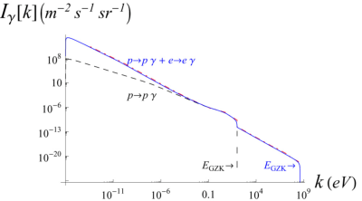
As mentioned above these expressions are only indicative and assume constant average values for the age of a cosmic ray (either proton or electron). For a more detailed discussion we encourage the reader to examine our recent paper [16]. From this latter work we include the following figure describing the radiation yield
5 Conclusions and Outlook
In this work, the effect on charged particles of a mildly (compared to the particle momentum) time dependent pseudoscalar background has been investigated. We have been interested both in proton and electron cosmic rays.
This effect is calculable because the axion background induces a modification of QED that is exactly solvable. This modification has some interesting features, such as the possibility of the photon emission process and (which we have termed as axion-induced Bremsstrahlung processes). Kinematical constraints on the process have been reviewed, in particular it is seen that it is only possible for proton energies higher than a certain threshold. The energy loss of protons in such a background has been computed. For protons that survive the GZK cutoff this loss is totally negligible.
However, the radiated photons could still be detected. Their flux and energy spectrum have been computed in some detail. Since the energy threshold depends on the mass of the charged particle, it is lower for lighter particles. Also, the energy loss is proportional to the mass squared of the charged particle, so the effect is more important for electrons. The value of does not depend on the charged particle mass, so the radiated spectrum is no very different for electrons or protons (however the average lifetime of electron and protons cosmic rays is quite different and this has an observable effect on the power spectrum of the radiation).
We refer the interested reader to [16] for a more comprehensive description of this phenomenon and on the possibility of this diffuse radiation being measured. We summarize however the main conclusions below.
The dominant contribution to the radiation yield via this mechanism comes from electron (and positron) cosmic rays. If one assumes that the power spectrum of the cosmic rays is characterized by an exponent then the produced radiation has an spectrum for proton primaries, which becomes for electron primaries. The dependence on the key parameter comes with the exponent and for protons and electrons, respectively. However for the regions where the radiation yield is largest electrons amply dominate. We have assumed that the flux of electron cosmic rays is uniform throughout the Galaxy and thus identical to the one observed in our neighbourhood, but relaxing this hypothesis could provide an enhancement of the effect by a relatively large factor. The effect for the lowest wavelengths where the atmosphere is transparent and for values of corresponding to the current experimental limit is of mJy. This is at the limit of sensitivity of antenna arrays that are already currently being deployed and thus a possibility worth exploring.
In the case of radiation originating from our galaxy the main unknown in the present discussion is whether the flux of electron cosmic rays measured in our neighbourhood is representative of the Galaxy or not. Since it is possible to relate this flux to the galactic synchrotron radiation one could deduce the former from measuring the latter. It appears[17] that either the total number of electron cosmic rays is substantially larger than the one measured in the solar system, or the galactic magnetic fields have to stronger than expected. This issue remains to be further quantified. No attempt has been made to quantify the signal from possible extragalactic sources either.
One should note that the effect discussed here is a collective one. This is at variance with the GZK effect alluded in the first section - the CMB radiation is not a coherent one over large scales. For instance, no similar effect exists for hot axions. A second observation is that some of the scales that play a role in the present discussion are somewhat non-intuitive (for instance the ’cross-over’ scale or the threshold scale ). This is due to the non Lorentz-invariant nature of this effect. Finally, it may look surprising at first that an effect that has such a low probability may give a small but not ridiculously small contribution. The reason why this happens is that the number of cosmic rays is huge. It is known that they contribute to the energy density of the Galaxy by an amount similar to the Galaxy’s magnetic field[18].
There are several aspects of the present analysis that could be improved to make it more precise, particularly a piecewise constant oscillating axion background, or one with a serrated time profile for that matter, could be solved easily without having to appeal to special functions (the sinus profile involves Mathieu functions). This will be presented elsewhere but the present analysis suffices to indicate the order of magnitude of the effect.
We hope that the present mechanism help to assess the presumed relevance of cold axions as a dark matter candidate.
Acknowledgements
We thank our collaborator F. Mescia who participated in the research reported here. We acknowledge the financial support from projects FPA2007-66665, 2009SGR502, Consolider CPAN CSD2007-00042 and FLAVIANET. We thank A. De Rújula for some comments on cosmic rays and, particularly, J.M. Paredes and P. Planesas for discussions concerning the Galaxy synchrotron radiation. D.E. would like to thank the organizers of the Quarks 2010 workshop in Kolomna for the warm hospitality extended to him.
References
- [1] L.Abbott and P. Sikivie, Phys. Lett. 120B, 133 (1983)
- [2] M. Kuster, G. Raffelt and B. Beltran (eds), Axions: Theory, Cosmology and Experimental Searches, Lecture Notes in Physics 741 (2008).
- [3] E. W. Kolb and M. S. Turner, The Early Universe (Westview Press, 1990); Y. Sofue and V. Rubin, Ann. Rev. Astron. Astrophys. 39, 137 (2001); S. J. Asztalos et al., Ap. Jour. 571, L27 (2002).
- [4] E.I. Gates, G. Gyruk and M.S. Turner, Ap. Jour. 449, L123 (1995)
- [5]
K. Greisen,
Phys. Rev. Lett. 16, 748 (1966);
G.T. Zatsepin, V. A. Kuz’min, Journal of Exp. and Th. Phys. Let. 4 (78), 201380. - [6]
R.D. Peccei, H.R. Quinn, Phys. Rev. Lett. 38 (1977) 1440.
S. Weinberg, Phys. Rev. Lett. 40 (1978) 223.
F. Wilzcek, Phys. Rev. Lett. 40 (1978) 279. - [7] M. Dine, W. Fischler and M. Srednicki, Phys. Lett. B, 104, 199 (1981); A.R. Zhitnitsky, Sov. J. Nucl. Phys. 31, 260 (1980).
- [8] J. E. Kim, Phys. Rev. Lett. 43, 103 (1979); M. A. Shifman, A. I. Vainshtein and V. I. Zakharov, Nucl. Phys. B 166, 493 (1980).
- [9] J. Abraham et al, (Pierre Auger Collaboration). arXiv:0906.2189v2
- [10] K. Nakamura et al. (Particle Data Group), J. Phys. G 37, 075021 (2010). M. Aguilar-Benitez et al [AMS-I Collaboration], Phys. Rep. 366, 331 (2002); M. Boezio et al. [CAPRICE Collaboration], Astrophys. J. 532, 653 (2000). See also the recent measurement by M. Ackermann et al [The FERMI LAT Collaboration], arXiv: 1008.3999v1, confirming previous estimates.
- [11] N. Kawanaka, K. Ioka and M. Nojiri, Astrophys. J. 710 (2010) 958.
- [12] A. Casadei and V. Bindi, in Proceedings of the 28th International Cosmic Ray Conference, Universal Academy Press, Tokyo, 2003.
- [13] C. Amsler et al. (Particle Data Group), PL B667, 1 (2008) and 2009 partial update for the 2010 edition
- [14] A. Andrianov, P. Giacconi and R. Soldati, JHEP 0202:030, 2002.
- [15] A. Andrianov, D. Espriu, P. Giacconi and R. Soldati, JHEP 0909:057, 2009.
- [16] D. Espriu, F. Mescia and A. Renau , arXiv:1010.2589
- [17] M.S. Longair, High Energy Astrophysics, vol. 2, Cambridge University Press, Cambridge (UK), 1994; B.F. Burke and F. Graham-Smith, ”An introduction to radio astronomy”, Cambridge University Press (Cambridge, UK), 1997; See also E. Orlando, Gamma rays from interactions of cosmic-ray electrons, Ph. D. Thesis (2008), http://www.imprs-astro.mpg.de/Alumni/Orlando-Elena.pdf.
- [18] See e.g.: A. Dar and A. De Rújula, Phys.Rept. 466,179 (2008).