Weakly directed self-avoiding walks

Axel Bacher Address: AB: LaBRI, Université Bordeaux 1, 351 cours de la Libération, 33405 Talence, France Email address: axel.bacher@labri.fr and Mireille Bousquet-Mélou Address: MBM: CNRS, LaBRI, Université Bordeaux 1, 351 cours de la Libération, 33405 Talence, France Email address: mireille.bousquet@labri.fr

Date: August 24, 2026

Abstract.

We define a new family of self-avoiding walks (SAW) on the square lattice, called weakly directed walks. These walks have a simple characterization in terms of the irreducible bridges that compose them. We determine their generating function. This series has a complex singularity structure and in particular, is not D-finite. The growth constant is approximately $2.54$ and is thus larger than that of all natural families of SAW enumerated so far (but smaller than that of general SAW, which is about 2.64). We also prove that the end-to-end distance of weakly directed walks grows linearly. Finally, we study a diagonal variant of this model.

Key words and phrases:

Enumeration – Self-avoiding walks

2000 Mathematics Subject Classification

05A15

1. Introduction

A lattice walk is self-avoiding if it never visits the same vertex twice (Fig. 1). Self-avoiding walks (SAW) have attracted interest for decades, first in statistical physics, where they are considered as polymer models, and then in combinatorics and in probability theory [25]. However, their properties remain poorly understood in low dimension, despite the existence of remarkable conjectures. See [25] for dimension 5 and above, and [7] for recent progresses in 4 dimensions.

Refer to caption — Figure 1. A self-avoiding walk on the square lattice, and a random SAW of length 1,000,000, constructed by Kennedy using a pivot algorithm [22].

On two-dimensional lattices, it is strongly believed that the number $c_{n}$ of $n$ -step SAW and the average end-to-end distance $D_{n}$ of these walks satisfy

c_{n}\sim\alpha\mu^{n}n^{\gamma}\quad\hbox{and}\quad D_{n}\sim\kappa n^{\nu}

(1)

where $\gamma=11/32$ and $\nu=3/4$ . Several independent, but so far not completely rigorous methods predict these values, like numerical studies [16, 29], comparisons with other models [8, 26], probabilistic arguments involving SLE processes [24], enumeration of SAW on random planar lattices [13]… The growth constant (or connective constant) $\mu$ is lattice-dependent. It has recently been proved to be $\sqrt{2+\sqrt{2}}$ for the honeycomb lattice [12], as predicted for almost 30 years, and might be another bi-quadratic number (approximately $2.64$ ) for the square lattice [21].

Given the difficulty of the problem, the study of restricted classes of SAW is natural, and probably as old as the interest in SAW itself. The rule of this game is to design new classes of SAW that have both:

–

a natural description (to be conceptually pleasant),
–

some structure (so that the walks can be counted, and their asymptotic properties determined).

This paper fits in this program: we define and count a new large class of SAW, called weakly directed walks.

The two simplest classes of SAW on the square lattice probably consist of directed and partially directed walks: a walk is directed if it involves at most two types of steps (for instance North and East), and partially directed if it involves at most three types of steps (Fig. 2(a-b)). Partially directed walks play a prominent role in the definition of our weakly directed walks. Among other solved classes, let us cite spiral SAW [27, 17] and prudent walks [4, 10, 9]. We refer again to Fig. 2 for illustrations. Each time such a new class is defined and solved, one compares its properties to (1): have we reached with this class a large growth constant? Is the end-to-end distance of the walks sub-linear?

At the moment, the largest growth constant (about $2.48$ ) is obtained with prudent SAW. However, this is beaten by certain classes whose description involves a (small) integer $k$ , like SAW confined to a strip of height $k$ [1, 32], or SAW consisting of irreducible bridges of length at most $k$ [20, 23]. The structure of these walks is rather poor, which makes them rather unattractive from a combinatorial viewpoint. In the former case, they are described by a transfer matrix (the size of which increases exponentially with the height of the strip); in the latter case, the structure is even simpler, since these walks are just arbitrary sequences of irreducible bridges of small length. In both cases, the generating function is rational. The growth constant increases with $k$ , providing better and better lower bounds on the growth constant of general SAW. The ability of solving these models for larger values of $k$ mostly relies on progress in computer power. Regarding asymptotic properties, almost all solved classes of SAW exhibit a linear end-to-end distance, with the exception of spiral walks, which are designed so as to wind around their origin. But there are very few such walks [17], as their growth constant is 1.

With the weakly directed walks of this paper, we reach a growth constant of about $2.54$ . These walks are defined in the next section. Their generating function is given in Section 5, after some preliminary results on partially directed bridges (Sections 3 and 4). This series turns out to be much more complicated that the generating functions of directed and partially directed walks, which are rational: we prove that it has a natural boundary in the complex plane, and in particular is not D-finite (that is, it does not satisfy any linear differential equation with polynomial coefficients). However, we are able to derive from this series certain asymptotic properties of weakly directed walks, like their growth constant and average end-to-end distance (which we find, unfortunately, to grow linearly with the length). Finally, we perform in Section 6 a similar study for a diagonal variant of weakly directed walks. Our intuition told us that this variant would give a larger growth constant, but we shall see that this is wrong. Section 7 discusses a few more points, including random generation.

An extended abstract of this paper appeared in the proceedings of the 2010 FPSAC conference [2].

2. Weakly directed walks: definition

Let us denote by N, E, S and W the four square lattice steps. All walks in this paper are self-avoiding, so that this precision will often be omitted. For any subset $\mathcal{S}$ of $\{{\sf N},{\sf E},{\sf S},{\sf W}\}$ , we say that a (self-avoiding) walk is an $\mathcal{S}$ -walk if all its steps lie in $\mathcal{S}$ . For instance, the first walk of Fig. 2 is a NE-walk, but also a NEW-walk. The second is a NEW-walk. We say that a SAW is directed if it involves at most two types of steps, and partially directed if it involves at most three types of steps.

The definition of weakly directed walks stems from the following simple observations:

(i)

between two visits to any given horizontal line, a NE-walk only takes E steps,
(ii)

between two visits to any given horizontal line, a NEW-walk only takes E and W steps.

Conversely, a walk satisfies (i) if and only if it is either a NE-walk or, symmetrically, a SE-walk. Similarly, a walk satisfies (ii) if and only if it is either a NEW-walk or, symmetrically, a SEW-walk. Conditions (i) and (ii) thus respectively characterize (up to symmetry) NE-walks and NEW-walks.

Definition 1.

A walk is weakly directed if, between two visits to any given horizontal line, the walk is partially directed (that is, avoids at least one of the steps N, E, S, W).

Examples are shown in Fig. 3.

Figure 3. Two weakly directed walks. The second one is a bridge, formed of 5 irreducible bridges. Observe that these irreducible bridges are partially directed.

We will primarily focus on the enumeration of weakly directed bridges. As we shall see, this does not affect the growth constant. A self-avoiding walk starting at $v_{0}$ and ending at $v_{n}$ is a bridge if all its vertices $v\not=v_{n}$ satisfy $h(v_{0})\leq h(v)<h(v_{n})$ , where $h(v)$ , the height of $v$ , is its ordinate. Concatenating two bridges always gives a bridge. Conversely, every bridge can be uniquely factored into a sequence of irreducible bridges (nonempty bridges that cannot be written as the product of two nonempty bridges). This factorization is obtained by cutting the walk above each horizontal line of height $n+1/2$ (with $n\in{\mathbb{Z}}$ ) that the walk intersects only once (Fig. 3, right). It is known that the growth constant of bridges is the same as that of general self-avoiding walks [25]. The fact that bridges can be freely concatenated makes them useful objects in the study of self-avoiding walks [18, 20, 23, 24, 25].

The following result shows that the enumeration of weakly directed bridges boils down to the enumeration of (irreducible) partially directed bridges. It will be extended to general walks in Section 5.

Proposition 2.

A bridge is weakly directed if and only if each of its irreducible bridges is partially directed (that is, avoids at least one of the steps N, E, S, W). In fact, this means that each of its irreducible bridges is a NES- or NSW-walk.

Proof.

The second condition (being NES or NSW) looks more restrictive than the first one (being partially directed), but it is easy to see that they are actually equivalent: no non-empty ESW-walk is a bridge, and the only irreducible bridges among NEW-walks consist of a sequence of horizontal steps, followed by a N step: thus they are NES- or NSW-walks.

So let us now consider a bridge whose irreducible bridges are partially directed. The portion of the walk lying between two visits to a given horizontal line is entirely contained in one irreducible bridge, and consequently, is partially directed.

Conversely, consider a weakly directed bridge and one of its irreducible bridges $w$ . Of course, $w$ is also weakly directed. Let $v_{0},\ldots,v_{n}$ be the vertices of $w$ , and let $s_{i}$ be the step that goes from $v_{i-1}$ to $v_{i}$ . We want to prove that $w$ is a NES- or NSW-walk. Assume that, on the contrary, $w$ contains a W step and an E step. By symmetry, we may assume that the first W occurs before the first E. Let $s_{k+1}$ be the first E step, and let $s_{j}$ be the last W step before $s_{k+1}$ . Then $s_{j+1},\ldots,s_{k}$ is a sequence of N or S steps. Let $h$ be the height of $s_{k+1}$ .

•

Assume that $s_{j+1},\ldots,s_{k}$ are N steps (first walk in Fig. 4). Let $h^{\prime}$ be the maximal height reached before $v_{j}$ , say at $v_{i}$ , with $i<j$ . Then $h^{\prime}<h$ (otherwise, between the first visit to height $h$ and $v_{k+1}$ , the walk would not be partially directed). Given that $w$ is irreducible, it must visit height $h^{\prime}$ again after $v_{k+1}$ , say at $v_{\ell}$ . But then the walk joining $v_{i}$ to $v_{\ell}$ is not partially directed, a contradiction.
•

Assume that $s_{j+1},\ldots,s_{k}$ are S steps (second walk in Fig. 4). Let $v_{i}$ , with $i<k$ , be the last visit at height $h$ before $v_{k}$ . Then the portion of the walk joining $v_{i}$ to $v_{k+1}$ is not partially directed, a contradiction.

Consequently, the irreducible bridge $w$ is a NES- or NSW-walk.

Figure 4. Illustrations for the proof of Proposition 2.

We discuss in Section 6 a variant of weakly directed walks, where we constrain the walk to be partially directed between two visits to the same diagonal line (Fig. 5). The notion of bridges is adapted accordingly, by defining the height of a vertex as the sum of its coordinates. We will refer to this model as the diagonal model, and to the original one as the horizontal model. There is, however, no simple counterpart of Proposition 2: a (diagonal) bridge whose irreducible bridges are partially directed is always weakly directed, but the converse is not true, as can be seen in Fig. 5. Thus bridges with partially directed irreducible bridges form a proper subclass of weakly directed bridges. We will enumerate this subclass, and study its asymptotic properties.

3. Partially directed bridges: a step-by-step approach

Let us equip the square lattice ${\mathbb{Z}}^{2}$ with its standard coordinate system. With each model (horizontal or diagonal) is associated a notion of height: the height of a vertex $v$ , denoted by $h(v)$ , is its ordinate in the horizontal model, and the sum of its coordinates in the diagonal model. Recall that a walk, starting at $v_{0}$ and ending at $v_{n}$ , is a bridge if all its vertices $v\not=v_{n}$ satisfy $h(v_{0})\leq h(v)<h(v_{n})$ . If the weaker inequality $h(v_{0})\leq h(v)\leq h(v_{n})$ holds for all $v$ , we say the walk is a pseudo-bridge. Note that nonempty bridges are obtained by adding a step of height $1$ to a pseudo-bridge (a N step in the horizontal model, a N or E step in the diagonal model). It is thus equivalent to count bridges or pseudo-bridges.

By Proposition 2, the enumeration of weakly directed bridges in the horizontal model boils down to the enumeration of (irreducible) partially directed bridges. In this section and the following one, we address the enumeration of these building blocks, first in a rather systematic way based on a step-by-step construction, then in a more combinatorial way based on heaps of cycles. A third approach is briefly discussed in the final section. We also count partially directed bridges in the diagonal model, which will be useful in Section 6.

As partially directed walks are defined by the avoidance of (at least) one step, there are four kinds of these. Hence, in principle, we should count, for each model (horizontal and diagonal), four families of partially directed bridges. However, in the horizontal model, there exists no non-empty ESW-bridge, and every NEW-walk is a pseudo-bridge. The latter class of walks is very easy to count, and has a rational generating function (Lemma 16). Moreover, a symmetry transforms NES-bridges into NSW-bridges, so that there is really one class of bridges that we need to count. In the diagonal model, we need to count ESW-bridges (which are equivalent to NSW-bridges by a diagonal symmetry) and NES-bridges (which are equivalent to NEW-bridges). Finally, to avoid certain ambiguities, we need to count ES-bridges, but this has already been done in [6].

From now on, the starting point of our walks is always at height $0$ . The height of a walk is then defined to be the maximal height reached by its vertices.

3.1. NES-bridges in the horizontal model

Proposition 3.

Let $k\geq 0$ . In the horizontal model, the length generating function of NES-pseudo-bridges of height $k$ is

B^{(k)}(t)=\frac{t^{k}}{G_{k}(t)},

where $G_{k}(t)$ is the sequence of polynomials defined by

G_{-1}=1,\quad G_{0}=1-t,\quad\hbox{and for }k\geq 0,\quad G_{k+1}=(1-t+t^{2}+t^{3})G_{k}-t^{2}G_{k-1}.

Equivalently,

\sum_{k\geq 0}\frac{v^{k}t^{k}}{B^{(k)}(t)}=\sum_{k\geq 0}v^{k}G_{k}=\frac{1-t-t^{2}v}{1-(1-t+t^{2}+t^{3})v+t^{2}v^{2}},

(2)

B^{(k)}(t)=\frac{U-\bar{U}}{\bigl((1-t)U-t\bigr)U^{k}-\bigl((1-t)\bar{U}-t\bigr)\bar{U}^{k}},

where

U={\frac{1-t+{t}^{2}+{t}^{3}-\sqrt{\left(1-t^{4}\right)\left(1-2t-{t}^{2}\right)}}{2t}}

is a root of $t{u}^{2}-\left(1-t+{t}^{2}+{t}^{3}\right)u+t=0$ and $\bar{U}:=1/U$ is the other root of this polynomial.

Proof.

Fix $k\geq 0$ . Let $\mathcal{T}$ be the set of NES-walks that end with an E step, and in which each vertex $v$ satisfies $0\leq h(v)\leq k$ . Let $\mathcal{T}_{i}$ be the subset of $\mathcal{T}$ consisting of walks that end at height $i$ . Let $T_{i}(t)\equiv T_{i}$ be the length generating function of $\mathcal{T}_{i}$ , and define the bivariate generating function

T(t;u)\equiv T(u)=\sum_{i=0}^{k}T_{i}(t)u^{i}.

This series counts walks of $\mathcal{T}$ by their length and the height of their endpoint. Note that we often omit the variable $t$ in our notation. The walks of $\mathcal{T}_{k}$ are obtained by adding an E step at the end of a pseudo-bridge of height $k$ , and hence $B^{(k)}(t)=T_{k}(t)/t$ . Alternatively, pseudo-bridges of height $k$ containing at least one E step are obtained by adding a sequence of N steps of appropriate length to a walk of $\mathcal{T}$ , and this gives

B^{(k)}(t)=t^{k}+\sum_{i=0}^{k}T_{i}(t)t^{k-i}=t^{k}\left(1+T(1/t)\right).

(3)

(The term $t^{k}$ accounts for the walk formed of $k$ consecutive N steps.)

Lemma 4.

The series $T(t;u)$ , denoted $T(u)$ for short, satisfies the following equation:

\left(1-\frac{ut^{2}}{1-tu}-\frac{t}{1-t\bar{u}}\right)T(u)=t\,\frac{1-(tu)^{k+1}}{1-tu}-t\,\frac{(tu)^{k+1}}{1-tu}T(1/t)-\frac{t^{2}\bar{u}}{1-t\bar{u}}T(t),

with $\bar{u}=1/u$ .

Proof.

We partition the set $\mathcal{T}$ into three disjoint subsets, illustrated in Fig. 7.

•

The first subset consists of walks with a single E step. These walks read ${\sf N}\cdots{\sf N}{\sf E}$ , with at most $k$ occurrences of N, and their generating function is

$t\sum_{i=0}^{k}(tu)^{i}=t\,\frac{1-(tu)^{k+1}}{1-tu}.$

•

The second subset consists of walks in which the last E step is strictly higher than the previous one. Denoting by $i$ the height of the next-to-last E step, the generating function of this subset reads

t\,\sum_{i=0}^{k}\left(T_{i}(t)u^{i}\sum_{j=1}^{k-i}(tu)^{j}\right)=t\,\sum_{i=0}^{k}\left(T_{i}(t)u^{i}\,\frac{tu-(tu)^{k-i+1}}{1-tu}\right)=\frac{ut^{2}}{1-tu}T(u)-t\,\frac{(tu)^{k+1}}{1-tu}T(1/t).

•

The third subset consists of walks in which the last E step is weakly lower than the previous one. Denoting by $i$ the height of the next-to-last E step, the generating function of this subset reads

t\,\sum_{i=0}^{k}\left(T_{i}(t)u^{i}\sum_{j=0}^{i}(t\bar{u})^{j}\right)=t\,\sum_{i=0}^{k}\left(T_{i}(t)u^{i}\,\frac{1-(t\bar{u})^{i+1}}{1-t\bar{u}}\right)=\frac{t}{1-t\bar{u}}T(u)-\frac{t^{2}\bar{u}}{1-t\bar{u}}T(t).

Adding the three contributions gives the series $T(u)$ and establishes the lemma.

Figure 7. Recursive construction of bounded NES-walk in the horizontal model.

The equation of Lemma 4 is easily solved using the kernel method (see e.g. [3, 5, 28]). The kernel of the equation is the coefficient of $T(u)$ , namely

1-\frac{ut^{2}}{1-tu}-\frac{t}{1-t\bar{u}}.

It vanishes when $u=U$ and $u=\bar{U}:=1/U$ , where $U$ is defined in the lemma. Since $T(u)$ is a polynomial in $u$ , the series $T(U)$ and $T(\bar{U})$ are well-defined. Replacing $u$ by $U$ or $\bar{U}$ in the functional equation cancels the left-hand side, and hence the right-hand side. One thus obtains two linear equations between $T(t)$ and $T(1/t)$ :

	$\displaystyle 0$	$\displaystyle=$	$\displaystyle t\,\frac{1-(tU)^{k+1}}{1-tU}-t\,\frac{(tU)^{k+1}}{1-tU}T(1/t)-\frac{t^{2}\bar{U}}{1-t\bar{U}}T(t),$
	$\displaystyle 0$	$\displaystyle=$	$\displaystyle t\,\frac{1-(t\bar{U})^{k+1}}{1-t\bar{U}}-t\,\frac{(t\bar{U})^{k+1}}{1-t\bar{U}}T(1/t)-\frac{t^{2}U}{1-tU}T(t).$

Solving this system gives in particular the value of $T(1/t)$ , and thus of $B^{(k)}(t)$ (thanks to (3)). This provides the second expression of $B^{(k)}(t)$ given in Proposition 3. The other results easily follow, using standard connections between linear recurrence relations, their solutions, and rational generating functions [30, Thm. 4.1.1].

3.2. ESW-bridges in the diagonal model

Proposition 5.

Let $k\geq 0$ . In the diagonal model, the length generating function of ESW-pseudo-bridges of height $k$ is

B_{1}^{(k)}(t)=\frac{t^{k}}{G_{k}(t)},

where $G_{k}(t)$ is the sequence of polynomials defined by

G_{0}=1,\quad G_{1}=1-t^{2}\quad\hbox{and for }k\geq 1,\quad G_{k+1}=(1+t^{2})G_{k}-t^{2}(2-t^{2})G_{k-1}.

Equivalently,

\sum_{k\geq 0}\frac{v^{k}t^{k}}{B_{1}^{(k)}(t)}=\sum_{k\geq 0}v^{k}G_{k}=\frac{1-2t^{2}v}{1-(1+t^{2})v+t^{2}(2-t^{2})v^{2}},

B_{1}^{(k)}(t)=\frac{U-(2-t^{2})\bar{U}}{(U-2t)U^{k}-\bigl((2-t^{2})\bar{U}-2t\bigr)\bigl((2-t^{2})\bar{U}\bigr)^{k}},

where

U={\frac{1+{t}^{2}-\sqrt{\left(1-t^{2}\right)\left(1-5\,{t}^{2}\right)}}{2t}}

is a root of $t{u}^{2}-\left(1+{t}^{2}\right)u+t\left(2-{t}^{2}\right)=0$ and $\bar{U}:=1/U$ .

Proof.

The proof is very close to the proof of Proposition 3, but the role that was played by E steps is now played by S steps. In particular, $\mathcal{T}$ is now the set of ESW-walks that end with a S step, and in which each vertex $v$ satisfies $0\leq h(v)\leq k$ . The sets $\mathcal{T}_{i}$ and the series $T_{i}(t)\equiv T_{i}$ and $T(t;u)\equiv T(u)$ are then defined in terms of $\mathcal{T}$ as before. Note that $T_{k}$ is in fact $0$ .

Pseudo-bridges of height $k$ containing at least one S step are obtained by adding a sequence of E steps of appropriate length to a walk of $\mathcal{T}$ , and (3) still holds (with $B^{(k)}$ replaced by $B_{1}^{(k)}$ ).

Lemma 6.

The series $T(t;u)$ , denoted $T(u)$ for short, satisfies the following equation:

\left(1-\frac{t^{2}}{1-tu}-\frac{t\bar{u}}{1-t\bar{u}}\right)T(u)=t^{2}\,\frac{1-(tu)^{k}}{1-tu}-t^{2}\,\frac{(tu)^{k}}{1-tu}T(1/t)-\frac{t\bar{u}}{1-t\bar{u}}T(t),

with $\bar{u}=1/u$ .

Proof.

We partition the set $\mathcal{T}$ into three disjoint subsets.

•

The first subset consists of walks with a single S step. Their generating function is

$t\bar{u}\sum_{i=1}^{k}(tu)^{i}=t^{2}\,\frac{1-(tu)^{k}}{1-tu}.$

•

The second subset consists of walks in which the last S step is weakly higher than the previous one. Their generating function reads

t\bar{u}\,\sum_{i=0}^{k}\left(T_{i}(t)u^{i}\sum_{j=1}^{k-i}(tu)^{j}\right)=\frac{t^{2}}{1-tu}T(u)-t^{2}\,\frac{(tu)^{k}}{1-tu}T(1/t).

•

The third subset consists of walks in which the last S step is strictly lower than the previous one. Their generating function reads

t\bar{u}\,\sum_{i=0}^{k}\left(T_{i}(t)u^{i}\sum_{j=0}^{i-1}(t\bar{u})^{j}\right)=\frac{t\bar{u}}{1-t\bar{u}}T(u)-\frac{t\bar{u}}{1-t\bar{u}}T(t).

Adding the three contributions establishes the lemma.

Again, we solve the equation of Lemma 6 using the kernel method, and conclude the proof of Proposition 5 using (3) (with $B^{(k)}$ replaced by $B_{1}^{(k)}$ ).

3.3. NES-bridges in the diagonal model

The generating function of NES-pseudo bridges is closely related to that of ESW-pseudo-bridges. This will be explained combinatorially in Section 7, after a detour via partially directed excursions.

Proposition 7.

Let $k\geq 0$ . In the diagonal model, the length generating function of NES-pseudo-bridges of height $k$ is

B_{2}^{(k)}(t)=\frac{t^{k}(2-t^{2})^{k}}{G_{k}(t)},

where $G_{k}(t)$ is the sequence of polynomials defined in Proposition 5. In other words,

B_{2}^{(k)}(t)={(2-t^{2})^{k}}B_{1}^{(k)}(t),

so that other expressions of $B_{2}^{(k)}(t)$ can be derived from Proposition 5.

Proof.

The sets $\mathcal{T}$ , $\mathcal{T}_{i}$ , and the corresponding series $T_{i}(t)\equiv T_{i}$ and $T(t;u)\equiv T(u)$ are defined as in the proof of Proposition 3 — only, the notion of height has changed. Note that $T_{0}$ is $0$ .

Pseudo-bridges of height $k$ containing at least one E step are again obtained by adding a sequence of N steps of appropriate length to a walk of $\mathcal{T}$ , and (3) still holds (with $B^{(k)}$ replaced by $B_{2}^{(k)}$ ).

Lemma 8.

The series $T(t;u)$ , denoted $T(u)$ for short, satisfies the following equation:

\left(1-\frac{ut}{1-tu}-\frac{t^{2}}{1-t\bar{u}}\right)T(u)=tu\,\frac{1-(tu)^{k}}{1-tu}-\frac{(tu)^{k+1}}{1-tu}T(1/t)-\frac{t^{2}}{1-t\bar{u}}T(t),

with $\bar{u}=1/u$ .

Proof.

We partition the set $\mathcal{T}$ into three disjoint subsets, defined as in the proof of Lemma 4.

•

The first subset consists of walks with a single E step. Their generating function is

$tu\sum_{i=0}^{k-1}(tu)^{i}=tu\,\frac{1-(tu)^{k}}{1-tu}.$

•

The second subset consists of walks in which the last E step is strictly higher than the previous one. Their generating function reads

tu\,\sum_{i=0}^{k}\left(T_{i}(t)u^{i}\sum_{j=0}^{k-i-1}(tu)^{j}\right)=\frac{ut}{1-tu}T(u)-\frac{(tu)^{k+1}}{1-tu}T(1/t).

•

The third subset consists of walks in which the last E step is weakly lower than the previous one. Their generating function reads

tu\,\sum_{i=0}^{k}\left(T_{i}(t)u^{i}\sum_{j=1}^{i}(t\bar{u})^{j}\right)=\frac{t^{2}}{1-t\bar{u}}T(u)-\frac{t^{2}}{1-t\bar{u}}T(t).

Adding the three contributions establishes the lemma.

The kernel occurring in Lemma 8 is obtained by replacing $u$ by $\bar{u}$ in the kernel of Lemma 6. Consequently, it vanishes when $u=1/U$ or $u=U/(2-t^{2})$ , where $U$ is the series defined in Proposition 5. We use the kernel method to solve the equation of Lemma 8, and conclude the proof of Proposition 7 using (3) (with $B^{(k)}$ replaced by $B_{2}^{(k)}$ ).

3.4. ES-bridges in the diagonal model

We state our last result on partially directed bridges without proof, for two reasons. Firstly, the step-by-step approach used in the previous subsections should have become routine by now, and is especially simple to implement here. Secondly, this result already appears in [6, Prop. 3.1] (where a bridge preceded by an E step is called a culminating path).

Proposition 9.

Let $k\geq 0$ . In the diagonal model, the length generating function of ES-pseudo-bridges of height $k$ is

B_{0}^{(k)}(t)=\frac{t^{k}}{F_{k}(t)},

where $F_{k}(t)$ is the sequence of polynomials defined by

F_{-1}=1,\quad F_{0}=1,\quad\hbox{and for }k\geq 0,\quad F_{k+1}=F_{k}-t^{2}F_{k-1}.

Equivalently,

\sum_{k\geq 0}\frac{v^{k}t^{k}}{B_{0}^{(k)}(t)}=\sum_{k\geq 0}v^{k}F_{k}={\frac{1-v{t}^{2}}{1-v+{v}^{2}{t}^{2}}},

B_{0}^{(k)}(t)=\frac{U^{2}-\bar{U}^{2}}{U^{k+2}-\bar{U}^{k+2}},

where

U=\frac{1-\sqrt{1-4t^{2}}}{2t}

is a root of $tu^{2}-u+t=0$ and $\bar{U}:=1/U$ is the other root of this polynomial.

4. Partially directed bridges via heaps of cycles

In this section, we give alternative (and more combinatorial) proofs of the results of Section 3. In particular, these proofs explain why the numerators of the rational series that count partially directed bridges of height $k$ are so simple ( $t^{k}$ or $t^{k}(2-t^{2})^{k}$ , depending on the model).

As a preliminary observation, let us note that ES-pseudo-bridges of height $k$ in the diagonal model can be seen as arbitrary paths on the segment $\{0,1,\ldots,k\}$ , with steps $\pm 1$ , going from $0$ to $k$ . Therefore, a natural way to count them is to use a classical result that expresses the generating function of paths with prescribed endpoints in a directed graph. This result is recalled in Proposition 10 below. It gives a straightforward proof of Proposition 9. However, the other three classes of bridges that we have counted do not fall immediately in the scope of this general result, because of the self-avoidance condition (which holds automatically for ES-walks). For instance, in the horizontal model, a NES-pseudo-bridge of height $k$ is not an arbitrary path with steps $0,\pm 1$ going from $0$ to $k$ on the segment $\{0,1,\ldots,k\}$ . We show here how to recover the results of Section 3 by factoring bridges into more general steps, and then applying Proposition 10.

Let $\Gamma=(V,E)$ be a (finite) directed graph. To each arc of this graph, we associate a weight taken in some commutative ring (typically, a ring of formal power series). A cycle of $\Gamma$ is a path ending at its starting point, taken up to a cyclic permutation. A path is self-avoiding if it does not visit the same vertex twice. A (non-empty) self-avoiding cycle is called an elementary cycle. Two paths are disjoint if their vertex sets are disjoint. The weight $w(\pi)$ of a path (or cycle) $\pi$ is the product of the weights of its arcs. A configuration of cycles $\gamma=\{\gamma_{1},\dotsc,\gamma_{r}\}$ is a set of pairwise disjoint elementary cycles. The signed weight of $\gamma$ is

\widetilde{w}(\gamma):=(-1)^{r}\prod_{i=1}^{r}w(\gamma_{i}).

For two vertices $i$ and $j$ , denote by $W_{i,j}$ the generating function of paths going from from $i$ to $j$ :

W_{i,j}=\sum_{\pi:i\leadsto j}w(\pi).

We assume that this sum is well-defined, which is always the case when $W_{i,j}$ is a length generating function.

Proposition 10.

The generating function of paths going from $i$ to $j$ in the weighted digraph $\Gamma$ is

W_{i,j}=\frac{N_{i,j}}{G}\text{,}

where $G=\sum_{\gamma}\widetilde{w}(\gamma)$ is the signed generating function of configuration of cycles, and

N_{i,j}=\sum_{\eta,\gamma}w(\eta)\widetilde{w}(\gamma)\text{,}

where $\eta$ is a self-avoiding path going from $i$ to $j$ and $\gamma$ is a configuration of cycles disjoint from $\eta$ .

This classical result can be proved as follows: one first identifies $W_{i,j}$ as the $(i,j)$ coefficient of the matrix $(1-A)^{-1}$ , where $A$ is the weighted adjacency matrix of $\Gamma$ . Thanks to standard linear algebra, this coefficient can be expressed in terms of the determinant of $(1-A)$ and one of its cofactors [30, Thms. 4.7.1 and 4.7.2]. A simple expansion of these as sums over permutations shows that the determinant is $G$ , and the cofactor $N_{i,j}$ . Proposition 10 can also be proved without any reference to linear algebra, using the theory of partially commutative monoids, or, more geometrically, heaps of pieces [15, 31]. In this context, configurations of cycles are called trivial heaps of cycles. This is the only justification of the title of this section, where no non-trivial heap will actually be seen.

As a straightforward application, let us sketch a second proof of Proposition 9. The vertices of $\Gamma$ are $0,1,\ldots,k$ , with an arc from $i$ to $j$ if $|i-j|=1$ . We apply the above proposition to count paths going from $0$ to $k$ . All arc weights are $t$ . The elementary cycles have length 2, and by induction on $k$ , it is easy to see that $G$ , the signed generating function of configurations of cycles, is the polynomial $F_{k}$ . The only self-avoiding path $\eta$ going from $0$ to $k$ consists of $k$ ‘up’ steps and visits all vertices, so that $N_{0,k}=t^{k}$ . Proposition 9 follows.

4.1. Bridges with large down steps

The proof of Proposition 9 that we have just sketched can be extended to paths with arbitrary large down steps. This will be used below to count partially directed bridges.

Let $\Gamma_{k}$ be the graph with vertices $\{0,\dotsc,k\}$ and with the following weighted arcs:

•

ascending arcs $i\to i+1$ of height $1$ , with weight $A$ , for $i=0,\ldots,k-1$ ;
•

descending arcs $i\to i-h$ of height $h$ , with weight $D_{h}$ , for $i=h,\ldots,k$ and $h\geq 0$ .

For $k\geq 0$ , denote by $C^{(k)}$ the generating function of paths from $0$ to $k$ in the graph $\Gamma_{k}$ . These paths may be seen as pseudo-bridges of height $k$ with general down steps.

Lemma 11.

The generating function of pseudo-bridges of height $k$ is

C^{(k)}=\frac{A^{k}}{H_{k}},

where the generating function of the denominators $H_{k}$ is

\sum_{k\geq 0}H_{k}v^{k}=\frac{1-D(vA)}{1-v+vD(vA)},

(4)

with $D(v)$ the generating function of descending steps:

D(v)=\sum_{h\geq 0}D_{h}v^{h}.

Proof.

With the notation of Proposition 10, the series $C^{(k)}$ reads $N_{0,k}/G$ . Since all ascending arcs have height 1, the only self-avoiding path from $0$ to $k$ consists of $k$ ascending arcs, and has weight $A^{k}$ . As it visits every vertex of the graph, the only configuration of cycles disjoint from it is the empty configuration. Therefore, the numerator $N_{0,k}$ is simply $A^{k}$ . The elementary cycles consist of a descending step of height, say, $h$ , followed by $h$ ascending steps. The weight of this cycle is $D_{h}A^{h}$ .

To underline the dependence of our graph in $k$ , denote by $H_{k}$ the denominator $G$ of Proposition 10. Consider a configuration of cycles of $\Gamma_{k}$ : either the vertex $k$ is free, or it is occupied by a cycle; this gives the following recurrence relation, valid for $k\geq 0$ :

H_{k}=H_{k-1}-\sum_{h=0}^{k}D_{h}A^{h}H_{k-h-1},

with the initial condition $H_{-1}=1$ . This is equivalent to (4).

4.2. Partially directed self-avoiding walks as arbitrary paths

As discussed above, it is not straightforward to apply Proposition 10 (or Lemma 11) to the enumeration of partially directed bridges, because of the self-avoidance condition. To circumvent this difficulty, we will first prove that partially directed self-avoiding walks are arbitrary paths on a line with large down steps.

It will be convenient to regard lattice walks as words on the alphabet $\{{\sf N},{\sf E},{\sf S},{\sf W}\}$ , and sets of walks as languages. We thus use some standard notation from the theory of formal languages [19]. The length of a word $u$ (the number of letters) is denoted by $|u|$ , and the number of occurrences of the letter $a$ in $u$ is $|u|_{a}$ . For two languages $\mathcal{L}$ and $\mathcal{L}^{\prime}$ ,

•

$\mathcal{L}+\mathcal{L}^{\prime}$ denotes the union of $\mathcal{L}$ and $\mathcal{L}^{\prime}$ ;
•

$\mathcal{L}\mathcal{L}^{\prime}$ denotes the language formed of all concatenations of a word of $\mathcal{L}$ with a word of $\mathcal{L}^{\prime}$ ;
•

$\mathcal{L}^{*}$ denotes the language formed of all sequences of words of $\mathcal{L}$ ;
•

$\mathcal{L}^{+}$ denotes the language formed of all nonempty sequences of words of $\mathcal{L}$ .

Finally, for any letter $a$ , we denote by $a$ the elementary language $\{a\}$ . A regular expression is any expression obtained from elementary languages using the sum, product, star and plus operators. It is unambiguous if every word of the corresponding language has a unique factorization compatible with the expression. To take a simple example, the expressions $({\sf N}+{\sf E})^{*}$ and $({\sf N}+{\sf W})^{*}$ are unambiguous expressions describing NE- and NW-walks respectively. However, the expression $({\sf N}+{\sf E})^{*}+({\sf N}+{\sf W})^{*}$ is ambiguous, as every N-walk is matched twice. Unambiguous regular expressions translate directly into enumerative results.

Let us say that a NES-walk is proper if it neither begins nor ends with a S step. All NES-pseudo-bridges are proper, whether in the horizontal or diagonal model. The following lemma explains how to see proper NES-walks as sequences of generalized steps.

Lemma 12.

Every proper NES-walk has a unique factorization into N steps and nonempty proper ES-walks with no consecutive E steps. In other words, the language of proper NES-walks admits the following unambiguous regular expression:

\bigl({\sf N}+{\sf E}({\sf S}^{+}{\sf E})^{*}\bigr)^{*}.

Proof.

The factorization of proper NES-walks is exemplified in Fig. 8. Every N step is a factor, as well as every maximal ES-walk with no consecutive E steps.

A similar result holds for ESW-walks (which we need to study in the diagonal model), which are obtained by applying a quarter turn to NES-walks. Let us say that an ESW-walk is proper if it neither begins nor ends with a W step. After a rotation, Lemma 12 gives for the language of proper ESW-walks the following unambiguous description:

\bigl({\sf E}+{\sf S}({\sf W}^{+}{\sf S})^{*}\bigr)^{*}.

(5)

4.3. Partially directed bridges

We can now give new proofs of the results of Section 3, based on Lemma 11.

Second proof of Proposition 3. Thanks to Lemma 12, self-avoiding NES-pseudo-bridges of height $k$ can be seen as arbitrary pseudo-bridges of height $k$ (in the sense of Lemma 11) where N is the only ascending step (of height 1 and weight $t$ ), and all words of ${\sf E}({\sf S}^{+}{\sf E})^{*}$ are descending steps. Moreover, the weight of a descending step $u$ is $t^{|u|}$ and its height is $|u|_{\sf S}$ . Thus, with the notation of Lemma 11, $A=t$ and the generating function $D(v)$ of descending steps is derived from the regular expression ${\sf E}({\sf S}^{+}{\sf E})^{*}$ :

\displaystyle D(v)

\displaystyle=\frac{t}{1-\frac{t^{2}v}{1-tv}}.

Proposition 3, in the form (2), now follows from Lemma 11.

Second proof of Proposition 5. Thanks to (5), self-avoiding ESW-pseudo-bridges of height $k$ can be seen as arbitrary pseudo-bridges of height $k$ (in the sense of Lemma 11) where E is the only ascending step (of weight $t$ ), and all words of ${\sf S}({\sf W}^{+}{\sf S})^{*}$ are descending steps. Moreover, the weight of a descending step $u$ is $t^{|u|}$ and its height is $|u|$ . Thus, with the notation of Lemma 11, $A=t$ and the generating function $D(v)$ of descending steps is

D(v)=\frac{tv}{1-\frac{t^{2}v^{2}}{1-tv}}.

Proposition 5 now follows from Lemma 11.

Second proof of Proposition 7. Again, the description of NES-walks given by Lemma 12 allows us to regard these self-avoiding walks as arbitrary paths with generalized steps. In the diagonal framework, the ascending steps $u$ are ${\sf N}$ and all words of ${\sf E}({\sf S}{\sf E})^{*}$ . They all have weight $t^{|u|}$ . All other words of ${\sf E}({\sf S}^{+}{\sf E})^{*}$ are descending. Moreover, the weight of a descending step $u$ is $t^{|u|}$ and its height is $|u|_{\sf S}-|u|_{\sf E}$ . Thus, with the notation of Lemma 11,

A=t+\frac{t}{1-t^{2}}=\frac{t(2-t^{2})}{1-t^{2}}\quad\hbox{and}\quad D(v)=\frac{tv^{-1}}{1-\frac{t^{2}}{1-tv}}-\frac{tv^{-1}}{1-t^{2}}.

However, one must pay attention to the following detail: in a NES-pseudo-bridge of height $k$ , only the last generalized step can end at height $k$ , because all descending steps begin with E. Similarly, all descending steps end with E, which implies that the only generalized step that starts at height $0$ is the first one (and moreover it is an ascending step). Thus a NES-pseudo-bridge of height $k\geq 2$ is really a pseudo-bridge (in the sense of Lemma 11) of height $k-2$ , preceded and followed by an ascending step. Thus for $k\geq 2$ ,

B_{2}^{(k)}=\frac{A^{k}}{H_{k-2}},

where the generating function of the denominators $H_{k}$ is given in Lemma 11. Given that $B_{0}^{(2)}=1$ and $B_{1}^{(2)}=A$ , we have

\sum_{k\geq 0}\frac{t^{k}(2-t^{2})^{k}v^{k}}{B^{(k)}_{2}(t)}=1+\frac{t(2-t^{2})v}{A}+\sum_{k\geq 2}\frac{t^{k}(2-t^{2})^{k}v^{k}}{A^{k}}H_{k-2}=\frac{1-2t^{2}v}{1-(1+t^{2})v+t^{2}(2-t^{2})v^{2}}.

This is equivalent to Proposition 7.

5. Weakly directed walks: the horizontal model

We now return to the weakly directed walks defined in Section 2. We determine their generating function, study their asymptotic number and average end-to-end distance, and finally prove that the generating function we have obtained has infinitely many singularities, and hence, cannot be D-finite.

5.1. Generating functions

By combining Propositions 2 and 3, it is now easy to count weakly directed bridges.

Proposition 13.

In the horizontal model, the generating function of weakly directed bridges is:

W(t)=\frac{1}{1+t-\frac{2tB}{1+tB}}

where $B:=\sum_{k\geq 0}B^{(k)}(t)$ is the generating function of NES-pseudo-bridges, given by Proposition 3.

Proof.

Let $\mathcal{I}_{\sf E}$ be the set of irreducible NES-bridges, and let $I_{\sf E}(t)$ be the associated length generating function. We will most of the time omit the variable $t$ in our series, writing for instance $I_{\sf E}$ instead of $I_{\sf E}(t)$ . Given that a non-empty NES-bridge is obtained by adding a N step at the end of a NES-pseudo-bridge, and is a (non-empty) sequence of irreducible NES-bridges, we have:

tB=\frac{I_{\sf E}}{1-I_{\sf E}}.

Define similarly the set $\mathcal{I}_{\sf W}$ , and the associated series $I_{\sf W}$ . By symmetry, $I_{\sf W}=I_{\sf E}$ . Moreover,

\mathcal{I}_{\sf E}\cap\mathcal{I}_{\sf W}={\sf N}.

Hence the generating function of irreducible bridges that are either NES or NSW is

I:=I_{\sf E}+I_{\sf W}-t=\frac{2tB}{1+tB}-t.

By Proposition 2, the generating function of weakly directed bridges is $W=\frac{1}{1-I}$ . The result follows.

We will now determine the generating function of (general) weakly directed walks. As we did for bridges, we factor them into “irreducible” factors, but the first and last factors are not necessarily bridges, so that we need to extend the notion of irreducibility to more general walks. Let us say that a walk $v_{0}\dotsm v_{n}$ is positive if all its vertices $v$ satisfy $h(v)\geq h(v_{0})$ , and that it is copositive if all vertices $v\neq v_{n}$ satisfy $h(v)<h(v_{n})$ . Thus a bridge is a positive and copositive walk.

Definition 14.

Let $r$ denote the reflection through the $x$ -axis. A non-empty walk $w$ is N-reducible if it is of the form $qp$ , where $q$ is a nonempty copositive walk and $p$ is a nonempty positive walk. It is S-reducible if $r(w)$ is N-reducible. Finally, it is irreducible if it is neither N-reducible nor S-reducible.

We can rephrase this definition as follows. If a horizontal line at height $h+1/2$ , with $h\in{\mathbb{Z}}$ , meets $w$ at exactly one point, we say that the step of $w$ containing this point is a separating step. Of course, this step is either N or S. Then a non-empty walk is irreducible if it does not contain any non-final separating step. It is then clear that the above definition extends the notion of irreducible bridges defined in Section 2: a non-empty bridge is never S-reducible, and it is N-reducible if and only if it is the product of two non-empty bridges. Also, observe that the endpoint of a N-reducible walk is strictly higher than its origin: Thus a walk may not be both N-reducible and S-reducible.

By cutting a walk after each separating step, one obtains a decomposition into a sequence of irreducible walks. This may be either a N-decomposition or a S-decomposition. The first factor of a N-decomposition is copositive, while the last one is positive. The intermediate factors are bridges.

We can now generalize Proposition 2, and characterize weakly directed walks in terms their irreducible factors.

Proposition 15.

A walk is weakly directed if and only if each of its irreducible factors is partially directed. Equivalently, each of these factors is a NES- or a NSW-walk.

Proof.

The proof is very similar to that of Proposition 2. First, the equivalence between the two conditions comes from the fact that any partially directed irreducible walk is NES or NSW.

Now, if all irreducible factors of a walk are partially directed, then this walk is weakly directed: two points of the walk lying on the same horizontal line belong to the same irreducible factor.

Conversely, let $w$ be an irreducible factor of a weakly directed walk; then $w$ is weakly directed. We prove that it is either a NES- or a NSW-walk. Assume that this is not the case, i.e. $w$ contains both a W and an E step. By symmetry, we may assume that it contains a W step before its first E step. By symmetry again, we may assume that, between the first E step and the last W step that precedes it, the walk consists of N steps. Then the first argument used in the proof of Proposition 2, depicted in the first part of Fig. 4, leads to a contradiction.

We now proceed to the enumeration of general weakly directed walks.

Lemma 16.

The generating functions $T(t)$ , $P(t)$ and $Q(t)$ of general, positive and copositive NES-walks are:

	$\displaystyle T(t)$	$\displaystyle=\frac{1+t}{1-2t-t^{2}},$
	$\displaystyle P(t)$	$\displaystyle=\frac{1}{2t^{2}}\Biggl(\sqrt{\frac{1-t^{4}}{1-2t-t^{2}}}-1-t\Biggr),$
	$\displaystyle Q(t)$	$\displaystyle=1+tP(t).$

Proof.

Let us start with general NES-walks. The language $\mathcal{T}$ of these walks is given by the following unambiguous description:

\mathcal{T}={\sf N}^{*}+{\sf S}^{+}+\mathcal{T}{\sf E}({\sf N}^{*}+{\sf S}^{+}),

from which the expression of $T(t)$ readily follows.

Let us now count positive walks. Let $P(t;u)$ be their generating function, with the variable $u$ accounting for the height of the endpoint. We decompose positive walks by cutting them before the last E step; this is similar to what we did in the proof of Lemma 4. We thus obtain:

P(t;u)=\frac{1}{1-tu}+\frac{t^{2}uP(t;u)}{1-tu}+\frac{t\bigl(P(t;u)-t\bar{u}P(t;t)\bigr)}{1-t\bar{u}}.

We rewrite this as follows:

\biggl(1-\frac{t^{2}u}{1-tu}-\frac{t}{1-t\bar{u}}\biggr)P(t;u)=\frac{1}{1-tu}-\frac{t^{2}\bar{u}P(t;t)}{1-t\bar{u}}.

We apply again the kernel method: we specialize $u$ to the series $U$ of Proposition 3; this cancels the coefficient of $P(t;u)$ , and we thus obtain the value of $P(t;t)$ . We then specialize the above equation to $u=1$ to determine $P(t;1)$ , which is the series denoted $P(t)$ in the lemma.

Finally, a non-empty copositive walk is obtained by reading a positive walk, seen as a word on $\{{\sf N},{\sf E},{\sf S},{\sf W}\}$ , from right to left, and adding a final N step. This gives the last equation of the lemma.

Proposition 17.

The generating function of weakly directed walks is

\overline{W}(t)=1+\bigl(2T_{i}(t)-2t\bigr)+2\bigl(2Q_{i}(t)-t\bigr)W(t)\bigl(2P_{i}(t)-t\bigr),

where the series $T_{i}(t)$ , $P_{i}(t)$ and $Q_{i}(t)$ count respectively general, positive, and copositive irreducible NES-walks, and are given by:

\displaystyle T_{i}(t)

\displaystyle=T(t)-1-2Q_{i}(t)\bigl(1+tB(t)\bigr)P_{i}(t),

\displaystyle P_{i}(t)

\displaystyle=\frac{P(t)-1}{1+tB(t)},

\displaystyle Q_{i}(t)

\displaystyle=\frac{Q(t)-1}{1+tB(t)}.

The series $W$ , $B$ , $T$ , $P$ and $Q$ are those of Proposition 13 and Lemma 16.

Proof.

In order to determine the series $T_{i}(t)$ , $P_{i}(t)$ and $Q_{i}(t)$ , we decompose into irreducible factors the corresponding families of NES-walks.

•
A general NES-walk is either
- –
  
  empty, or
- –
  
  irreducible, or
- –
  
  N-reducible: in this case, it consists of an irreducible copositive NES-walk, followed by a sequence of irreducible NES-bridges (forming a NES-bridge), and finally by an irreducible positive NES-walk; or
- –
  
  symmetrically, S-reducible.
Since $1+tB(t)$ is the generating function of bridges, this gives

$T(t)=1+T_{i}(t)+2Q_{i}(t)\bigl(1+tB(t)\bigr)P_{i}(t).$
•
We now specialize the above decomposition to positive NES-walks. Observe that when such a walk is N-reducible, its first factor is a bridge. This allows us to merge the second and third cases above. Moreover, the fourth case never occurs. Thus a positive NES-walk is either
- –
  
  empty, or
- –
  
  a NES-bridge followed by an irreducible positive NES-walk.
This yields:

$P(t)=1+\bigl(1+tB(t)\bigr)P_{i}(t).$
•
We proceed similarly for copositive NES-walks. Such a walk is either
- –
  
  empty, or
- –
  
  an irreducible copositive NES-walk followed by a NES-bridge.
This gives:

$Q(t)=1+Q_{i}(t)\bigl(1+tB(t)\bigr).$

We thus obtain the expressions of $T_{i}$ , $P_{i}$ and $Q_{i}$ announced in the proposition.

Recall from Proposition 15 that a walk is weakly directed if and only if its irreducible factors are NES- or NSW-walks. Thus,

•
a weakly directed walk is either
- –
  
  empty, or
- –
  
  an irreducible NES- or NSW-walk, or
- –
  
  N-reducible: it then factors into an irreducible copositive NES- or NSW-walk, a sequence of NES- or NSW- irreducible bridges (forming a weakly directed bridge), and an irreducible positive NES- or NSW-walk; or
- –
  
  symmetrically, S-reducible.

The contribution to $\overline{W}(t)$ of the first case is obviously 1. The only irreducible walks that are both NES and NSW are N and S. The generating function of irreducible NES- or NSW-walks is thus $2T_{i}(t)-2t$ . Similarly, the generating function of irreducible positive (resp. copositive) NES- or NSW-walks is $2P_{i}(t)-t$ (resp. $2Q_{i}(t)-t$ ). In both cases, the term $-t$ corresponds to the walk reduced to a N step, which is both NES and NSW. Adding the contributions of the four classes yields the announced expression of $\overline{W}(t)$ .

5.2. Asymptotic results

Proposition 18.

The generating function $W$ of weakly directed bridges, given in Proposition 13, is meromorphic in the disk $\mathcal{D}=\{z:|z|<\sqrt{2}-1\}$ . It has a unique dominant pole in this disk, $\rho\simeq 0.3929$ . This pole is simple. Consequently, the number $w_{n}$ of weakly directed bridges of length $n$ satisfies

w_{n}\sim\kappa\mu^{n},

with $\mu=1/\rho\simeq 2.5447$ .

Let $N_{n}$ denote the number of irreducible factors in a random weakly directed bridge of length $n$ . The mean and variance of $N_{n}$ satisfy:

\mathbb{E}(N_{n})\sim\mathfrak{m}\,n,\quad\quad\mathbb{V}(N_{n})\sim\mathfrak{s}^{2}\,n,

where

\mathfrak{m}\simeq 0.318\quad\hbox{and}\quad\mathfrak{s}^{2}\simeq 0.7,

and the random variable $\frac{N_{n}-\mathfrak{m}\,n}{\mathfrak{s}\sqrt{n}}$ converges in law to a standard normal distribution. In particular, the average end-to-end distance, being bounded from below by $\mathbb{E}(N_{n})$ , grows linearly with $n$ .

These results hold as well for general weakly directed walks, with other values of $\kappa$ , $\mathfrak{m}$ and $\mathfrak{s}$ .

Proof.

Recall from the proof of Proposition 13 that $W(t)=1/(1-I(t))$ , where $I(t)$ counts partially directed irreducible bridges, which are certain NES- or NSW-walks. The generating function $T(t)$ of NES-walks, given in Lemma 16, has radius of convergence $\sqrt{2}-1$ . Hence, $I$ has radius of convergence at least $\sqrt{2}-1$ , and $W$ is meromorphic in the disk $\mathcal{D}$ .

In this disk, we find a pole at each value of $t$ for which $I(t)=1$ . As $I(t)$ has non-negative coefficients and is aperiodic, a pole of minimal modulus, if it exists, can only be real, positive and simple. Thus if there is a pole in $\mathcal{D}$ , then $W$ has a unique dominant pole $\rho$ , which is simple, and the asymptotic behaviour of the numbers $w_{n}$ follows.

In order to prove the existence of $\rho$ , we use upper and lower bounds on the series $I(t)$ . For any series $F(t)=\sum_{m\geq 0}f_{m}t^{m}$ , and $n\geq 0$ , denote $F_{\leq n}(t):=\sum_{m=0}^{n}f_{m}t^{m}$ and $F_{>n}(t):=\sum_{m>n}f_{m}t^{m}$ . Then for $0<t<\sqrt{2}-1$ and $n\geq 0$ , we have

I^{-}(t)\leq I(t)\leq I^{+}(t),

(6)

where the series

I^{-}(t):=I_{\leq n}(t)\quad\hbox{ and }\quad I^{+}(t):=I_{\leq n}(t)+2T_{>n}(t)=I_{\leq n}(t)+2T(t)-2T_{\leq n}(t)

can be evaluated exactly for a given value of $n$ . The upper bound follows from the fact that $I$ counts walks that are either NES- or NSW-walks. Using these bounds, we can prove the existence of $\rho$ and locate it. More precisely,

\rho^{-}\leq\rho\leq\rho^{+},

(7)

where

I^{-}(\rho^{+})=I^{+}(\rho^{-})=1.

Taking $n=300$ gives 5 exact digits in $\mu=1/\rho$ .

Let us now study the number of irreducible bridges in a random weakly directed bridge. The series that counts these bridges by their length and the number of irreducible bridges is

W(t,x)=\frac{1}{1-xI(t)}.

(8)

One easily checks that $W(t,x)$ corresponds to a supercritical sequence, so that Prop. IX.7 of [14] applies and establishes the existence of a gaussian limit law, after standardization. Regarding the estimates of $\mathfrak{m}$ and $\mathfrak{s}$ , we have

\mathfrak{m}=\frac{1}{\rho I^{\prime}(\rho)}\quad\hbox{and}\quad\mathfrak{s}^{2}=\frac{I^{\prime\prime}(\rho)+I^{\prime}(\rho)-I^{\prime}(\rho)^{2}}{\rho I^{\prime}(\rho)^{3}}.

As $I(t)$ has non-negative coefficients, we can combine the bounds (6) on $I(t)$ and (7) on $\rho$ to obtain bounds on the values of $\mathfrak{m}$ and $\mathfrak{s}$ .

Consider now the generating function $\overline{W}$ of general weakly directed walks, given in Proposition 17. The series $T_{i}$ , $P_{i}$ and $Q_{i}$ count certain partially directed walks, and thus have radius at least $\sqrt{2}-1$ . Moreover, $2Q_{i}(t)-t>0$ and $2P_{i}(t)-t>0$ for $t>0$ . Hence $\overline{W}$ has, as $W$ itself, a unique dominant pole in $\mathcal{D}$ , which is $\rho$ .

The argument used to prove Proposition 17 shows that the series that counts weakly directed walks by their length and the number of irreducible factors is

\overline{W}(t,x)=1+x(2T_{i}(t)-2t)+2x^{2}(2Q_{i}(t)-t)W(t,x)(2P_{i}(t)-t),

where $W(t,x)$ is given by (8). This yields the announced results on the number of irreducible factors.

5.3. Nature of the series

Proposition 19.

The generating function $B=\sum_{k\geq 0}B^{(k)}(t)$ of NES-pseudo-bridges, given in Proposition 3, converges around $0$ and has a meromorphic continuation in ${\mathbb{C}}\setminus\mathcal{E}$ , where $\mathcal{E}$ consists of the two real intervals $[-\sqrt{2}-1,-1]$ and $[\sqrt{2}-1,1]$ , and of the curve

\mathcal{E}_{0}=\left\{x+iy:x\geq 0,\ {y}^{2}={\frac{1-{x}^{2}-2\,{x}^{3}}{1+2\,x}}\right\}.

This curve, shown in Fig. 9, is a natural boundary of $B$ . That is, every point of $\mathcal{E}_{0}$ is a singularity of $B$ .

The above statements hold as well for the generating function $W$ of weakly directed bridges, given in Proposition 13. In particular, neither $B$ nor $W$ is D-finite.

Before proving this proposition, let us establish two lemmas, dealing respectively with the series $U$ and the polynomials $G_{k}$ occurring in the expression of $B$ (Proposition 3).

Lemma 20.

For $t\in{\mathbb{C}}\setminus\{0\}$ , the equation $t(u+1/u)=1-t+t^{2}+t^{3}$ has two roots, counted with multiplicity. The product of these roots is $1$ . Their modulus is $1$ if and only if $t$ belongs to the set $\mathcal{E}$ defined in Proposition 19.

Let

U(t)={\frac{1-t+{t}^{2}+{t}^{3}-\sqrt{\left(1-t^{4}\right)\left(1-2t-{t}^{2}\right)}}{2t}}

be the root that is defined at $t=0$ . This series has radius of convergence $\sqrt{2}-1$ . It has singularities at $\pm\sqrt{2}-1$ , $\pm 1$ and $\pm i$ , and admits an analytic continuation in

{\mathbb{C}}\setminus\left([-\sqrt{2}-1,-1]\cup[\sqrt{2}-1,1]\cup[i,i\infty)\cup[-i,-i\infty)\right).

Proof.

The first two statements are obvious. Now assume that the roots $u$ and $1/u$ have modulus $1$ , that is, $u=e^{i\theta}$ for $\theta\in{\mathbb{R}}$ . This means that $f(t):=\frac{1-t+t^{2}+t^{3}}{2t}=\cos\theta$ is real, and belongs to the interval $[-1,1]$ . Write $t=x+iy$ , and express $\operatorname{Im}f(t)$ in terms of $x$ and $y$ . One finds that $f(t)$ is real if and only if either $y=0$ (that is, $t\in{\mathbb{R}}$ ) or

y^{2}(1+2x)=1-{x}^{2}-2\,{x}^{3}.

(9)

Since $y^{2}\geq 0$ , this is only possible if $-1/2<x\leq x_{c}$ where $x_{c}\sim 0.65...$ satisfies $1-{x}_{c}^{2}-2\,{x}_{c}^{3}=0$ . Observe that the above curve includes $\mathcal{E}_{0}$ .

For real values of $t$ , an elementary study of $f$ shows that $f(t)\in[-1,1]$ if and only if $t\in[-\sqrt{2}-1,-1]\cup[\sqrt{2}-1,1]$ (see Fig. 10, left). If $t=x+iy$ is non-real and (9) holds, then $f(t)={\frac{-1+4\,{x}^{2}+4\,{x}^{3}}{1+2\,x}}$ . Given that $-1/2<x\leq x_{c}$ , this belongs to $[-1,1]$ if and only if $x$ is non-negative (see Fig. 10, middle). We have thus proved that $|u|=1$ if and only if $t\in\mathcal{E}$ .

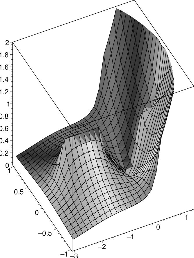
The properties of the series $U$ follow from basic complex analysis. Of course, one may choose the position of the cuts differently, provided they include the 6 singularities. With the cuts along the coordinate axes, a plot of the modulus of $U$ is shown on the right of Fig. 10.

Lemma 21.

Let $\mathcal{E}$ be the subset of ${\mathbb{C}}$ defined in Proposition 19, and $G_{k}$ the polynomials of Proposition 3.
If $G_{k}(z)=G_{\ell}(z)=0$ with $\ell\not=k$ , then $z\in\mathcal{E}$ .
If $G_{k}(z)=0$ and $z$ is non-real, then $z\not\in\mathcal{E}$ .
The set of accumulation points of roots of the polynomials $G_{k}$ is exactly $\mathcal{E}$ .

The latter point is illustrated in Fig. 9.

Proof.

Note first that, for $z\not=0$ ,

{G_{k}(z)}=z^{k}\ \frac{\bigl((1-z)u-z\bigr)u^{k}-\bigl((1-z)/u-z\bigr)u^{-k}}{u-1/u},

where $u$ and $1/u$ are the two roots of $z(u+1/u)=1-z+z^{2}+z^{3}$ .

Assume $G_{k}(z)=G_{\ell}(z)=0$ . Then $z\not=0$ (because $G_{k}(0)=1$ ). The equations $G_{k}(z)=G_{\ell}(z)=0$ imply $u^{2k}=u^{2\ell}$ , so that $|u|=1$ , that is, by Lemma 20, $z\in\mathcal{E}$ .

Assume $G_{k}(z)=0$ and $z$ is non-real. Assume moreover that $z\in\mathcal{E}$ . Let $u$ and $1/u$ be defined as above. By Lemma 20, $|u|=1$ . Write $u=e^{i\theta}$ . Then $G_{k}(z)=0$ implies

\frac{z}{1-z}=\frac{\sin((k+1)\theta)}{\sin(k\theta)},

which contradicts the assumption that $z$ is non-real.

Now let $z$ be an accumulation point of roots of the $G_{k}$ ’s. There exists a sequence $z_{i}$ that tends to $z$ such that $G_{k_{i}}(z_{i})=0$ , with $k_{i}\rightarrow\infty$ . We want to prove that $z\in\mathcal{E}$ . If $z$ is one of the 6 singularities of $U$ , then there is nothing to prove. Otherwise, $U$ has an analytic description in a neighborhood of $z$ . The equation $G_{k_{i}}(z_{i})=0$ reads

U(z_{i})^{2k_{i}}=\frac{(1-z_{i})/U(z_{i})-z_{i}}{(1-z_{i})U(z_{i})-z_{i}}.

By continuity, $U(z_{i})\rightarrow U(z)$ as $i\rightarrow\infty$ . If $z=0$ , then $U(z)=0$ and the right-hand side diverges while the left-hand side tends to $0$ . This is impossible, and hence $z\not=0$ . This implies that the right-hand side tends to a finite, non-zero limit and, by continuity, forces $|U(z)|=1$ . By Lemma 20, this means that $z\in\mathcal{E}$ .

Conversely, let $z\in\mathcal{E}$ . By Lemma 20, the two roots of $z(u+1/u)=1-z+z^{2}+z^{3}$ can be written $e^{\pm i\theta}$ . By density, we may assume that $\theta=j\pi/\ell$ , for $0<j<\ell$ . This excludes in particular the 6 singular points of $U$ , for which $u=\pm 1$ . This means that $U$ has an analytic description in a neighborhood of $z$ , so that for $t$ close to $z$ , $U(t)=U(z)(1+s)$ with $s=(t-z)\frac{U^{\prime}(z)}{U(z)}+O((t-z)^{2})$ . Thanks to the equation satisfied by $U(z)$ , it is easy to see that $U^{\prime}(z)\not=0$ if $z\not=x_{c}$ , where $x_{c}$ is defined in the proof of Lemma 20. We assume from now on that $z\not=x_{c}$ (again, by density, this is a harmless assumption). Let $k$ be a multiple of $\ell$ . The equation $G_{k}(t)=0$ reads

U(t)^{2k}=\frac{(1-t)/U(t)-t}{(1-t)U(t)-t},

or, given that $U(z)^{2k}=e^{2ijk\pi/\ell}=1$ ,

(1+s)^{2k}=\frac{(1-z)/U(z)-z}{(1-z)U(z)-z}+O(t-z).

The right-hand side being finite and non-zero, one finds a root $t$ of $G_{k}$ in the neighborhood of $z$ :

t=z+\frac{U(z)}{2kU^{\prime}(z)}\log\left(\frac{(1-z)/U(z)-z}{(1-z)U(z)-z}\right)+o(1/k),

and this root gets closer and closer to $z$ as $k$ increases. Thus $z$ is an accumulation point of roots of the $G_{k}$ ’s.

Proof of Proposition 19.
One has $B(t)=\sum t^{k}/G_{k}(t)$ , with

\frac{t^{k}}{G_{k}(t)}=\frac{u-1/u}{\bigl((1-t)u-t\bigr)u^{k}-\bigl((1-t)/u-t\bigr)u^{-k}},

(10)

$u$ and $1/u$ being the roots of $t(u+1/u)=1-t+t^{2}+t^{3}$ . Let us first prove that this series defines a meromorphic function in ${\mathbb{C}}\setminus\mathcal{E}$ . Assume $t\not\in\mathcal{E}$ . By Lemma 21, $t$ is not an accumulation point of roots of the polynomials $G_{k}$ , and cancels at most one of these polynomials. Hence there exists a neighborhood of $t$ in which at most one of the $G_{k}$ ’s has a zero, which is $t$ itself. Moreover, by Lemma 20, one of the roots $u$ and $1/u$ has modulus larger than $1$ . By continuity, this holds in a (possibly smaller) neighborhood of $t$ . Then (10) shows that the series $\sum t^{k}/G_{k}(t)$ is meromorphic in the vicinity of $t$ . Given that ${\mathbb{C}}\setminus\mathcal{E}$ is connected, we have proved that this series defines a meromorphic function in ${\mathbb{C}}\setminus\mathcal{E}$ . The same holds for $W(t)$ , which is a rational function of $t$ and $B(t)$ .

Let us now prove that $\mathcal{E}_{0}$ is a natural boundary of $B$ . By Lemma 21, every non-real zero of $G_{k}$ is in ${\mathbb{C}}\setminus\mathcal{E}$ , and does not cancel any other polynomial $G_{\ell}$ . Hence it is a pole of $B$ . Now let $z\in\mathcal{E}_{0}$ with $z\not\in{\mathbb{R}}$ . By Lemma 21, this point is an accumulation point of (non-real) zeroes of the polynomials $G_{k}$ , and thus an accumulation point of poles of $B$ . Thus it is a singularity of $B$ , and the whole curve $\mathcal{E}_{0}$ is a natural boundary of $B$ . Given that $B$ and $W$ are related by a simple homography, this curve is also a boundary for $W$ .

6. The diagonal model

We have defined weakly directed walks in the diagonal model by requiring that the portion of the walk joining two visits to the same diagonal is partially directed. This is analogous to the definition we had in the horizontal model. The definition of bridges is adapted accordingly, by defining the height of a vertex as the sum of its coordinates. However, there is no simple counterpart of Proposition 2: the irreducible bridges of a weakly directed bridge may not be partially directed (Fig. 5). However, it is easy to see that bridges formed of partially directed irreducible bridges are always weakly directed. In this section, we enumerate these walks and study their asymptotic properties.

6.1. Generating function

Proposition 22.

The generating function of bridges formed of partially directed irreducible bridges is

W_{\Delta}(t)=\frac{1}{1+2t-\displaystyle\frac{2tB_{1}}{1+tB_{1}}-\frac{4tB_{2}}{1+2tB_{2}}+\frac{2tB_{0}}{1+tB_{0}}},

where the series $B_{i}=\sum_{k\geq 0}B_{i}^{(k)}(t)$ are given in Propositions 5, 7, 9.

Proof.

Let $\mathcal{I}_{\sf S}$ be the set of irreducible ESW-bridges, and let $I_{\sf S}$ be the associated length generating function. Given that a non-empty ESW-bridge is obtained by adding an E step at the end of a ESW-pseudo-bridge, and a non-empty sequence of irreducible ESW-bridges, there holds

tB_{1}=\frac{I_{\sf S}}{1-I_{\sf S}}.

Define similarly the sets $\mathcal{I}_{\sf N}$ , $\mathcal{I}_{\sf E}$ and $\mathcal{I}_{\sf W}$ , and the associated series $I_{\sf N}$ , $I_{\sf E}$ and $I_{\sf W}$ . Finally, let $\mathcal{I}_{{\sf E}{\sf S}}$ (resp. $\mathcal{I}_{{\sf N}{\sf W}}$ ) be the set of irreducible ES-bridges (resp. NW-bridges), and let $I_{{\sf E}{\sf S}}$ (resp. $I_{{\sf N}{\sf W}}$ ) be the associated series. Then

2tB_{2}=\frac{I_{\sf E}}{1-I_{\sf E}}\quad\hbox{ and }\quad tB_{0}=\frac{I_{{\sf E}{\sf S}}}{1-I_{{\sf E}{\sf S}}}.

(The factor 2 comes from the fact that a NES-bridge may end with a N or E step.) By symmetry, $I_{\sf N}=I_{\sf E}$ , $I_{\sf W}=I_{\sf S}$ and $\mathcal{I}_{{\sf E}{\sf S}}=\mathcal{I}_{{\sf N}{\sf W}}$ . Moreover,

\mathcal{I}_{\sf S}\cap\mathcal{I}_{\sf N}={\sf E},\quad\mathcal{I}_{\sf S}\cap\mathcal{I}_{\sf E}=\mathcal{I}_{{\sf E}{\sf S}},\quad\mathcal{I}_{\sf S}\cap\mathcal{I}_{\sf W}=\emptyset,\quad\mathcal{I}_{\sf E}\cap\mathcal{I}_{\sf N}={\sf N}+{\sf E},\quad\mathcal{I}_{\sf E}\cap\mathcal{I}_{\sf W}={\sf N},\quad\mathcal{I}_{\sf W}\cap\mathcal{I}_{\sf N}=\mathcal{I}_{{\sf N}{\sf W}}.

By an elementary inclusion-exclusion argument, the generating function of partially directed irreducible bridges is

I:=2I_{\sf S}+2I_{\sf E}-2I_{{\sf E}{\sf S}}-2t=\frac{2tB_{1}}{1+tB_{1}}+\frac{4tB_{2}}{1+2tB_{2}}-\frac{2tB_{0}}{1+tB_{0}}-2t.

Hence the generating function of bridges formed of partially directed irreducible bridges is $W_{\Delta}=\frac{1}{1-I}$ . The result follows.

6.2. Asymptotic properties

We obtain for the diagonal model asymptotic results that are similar to those obtained in the horizontal model, with a slightly smaller growth constant. We have to confess that this contradicts our original intuition: since in the horizontal model, two of the four classes of irreducible partially directed bridges (namely, ESW and NEW) are either trivial or degenerate, while in the diagonal model, all four classes are non-trivial, we thought we had a chance to reach a better growth constant in the diagonal model. This is unfortunately not the case. We nonetheless present this diagonal variant, because we believe it to be a natural attempt. We analyze below what makes the difference between the two growth constants, and this analysis shows that our hopes could just as well have come true.

Proposition 23.

The generating function $W_{\Delta}$ given by Proposition 22 is meromorphic in the disk $\mathcal{D}=\{|z|<\sqrt{2}-1\}$ . It has a unique dominant pole in this disk, at $\rho_{1}\simeq 0.3940$ . This pole is simple. Consequently, the number of $n$ -step bridges formed of partially directed irreducible bridges is asymptotically equivalent to $\kappa\,{\mu}^{n}$ , with $\mu=1/\rho_{1}\simeq 2.5378$ .

Let $N_{n}$ denote the number of irreducible bridges in a random $n$ -step bridge formed of partially directed irreducible bridges. The mean and variance of $N_{n}$ satisfy:

\mathbb{E}(N_{n})\sim\mathfrak{m}\,n,\quad\quad\mathbb{V}(N_{n})\sim\mathfrak{s}^{2}\,n,

where

\mathfrak{m}\simeq 0.395\ \ \quad\hbox{and}\quad\mathfrak{s}^{2}=1\pm 2.10^{-3},

Proof.

The arguments are the same as in the proof of Proposition 18. This series reads $W_{\Delta}=1/(1-I)$ , where $I$ counts partially directed irreducible bridges. The only change is in the bounds we use on the series $I$ :

I^{-}(t)\leq I(t)\leq I^{+}(t),

with

I^{-}(t):=I_{\leq n}(t)\quad\hbox{ and }\quad I^{+}(t):=I_{\leq n}(t)+4T_{>n}(t)=I_{\leq n}(t)+4T(t)-4T_{\leq n}(t),

where $T(t)$ is the generating function of NES-walks, given in Lemma 16.

Remark. Hence the growth constant in the diagonal model is a bit smaller than in the horizontal model. This does not seem to be predictible. The series of Propositions 13 and 22 respectively read

W(t)=\frac{1}{1-I(t)}\quad\hbox{and}\quad W_{\Delta}(t)=\frac{1}{1-I_{\Delta}(t)}

where $I$ and $I_{\Delta}$ count irreducible partially directed bridges, respectively in the horizontal and diagonal model. As $t$ increases from $0$ to $\sqrt{2}-1$ (the radius of convergence of the series of partially directed walks), $I_{\Delta}(t)=2t+O(t^{2})$ first dominates $I(t)=t+O(t^{2})$ , but the graphs of these two functions cross before any of them reaches 1 (Fig. 11), so that $I(t)$ reaches 1 before $I_{\Delta}(t)$ does. The fact that the graphs cross is consistent with our belief that $I$ has radius $\sqrt{2}-1\sim 0.41$ while $I_{\Delta}$ has a larger radius of convergence, namely $1/\sqrt{5}\sim 0.44$ . But $I_{\Delta}(t)$ could just as well have reached 1 before the crossing point.

7. Final comments

7.1. One more way to count partially directed bridges

We have presented in Sections 3 and 4 two approaches to count partially directed bridges. Here, we discuss a third method, based on standard decompositions of lattice paths. This approach involves some guessing, whereas the two others don’t. In the diagonal model, it allows us to understand more combinatorially why the generating functions of NES- and ESW-bridges only differ by a factor $(2-t^{2})^{k}$ . Moreover, this approach is needed for random generation.

We first discuss the horizontal model, that is, the enumeration of NES-bridges given by Proposition 3. We say that a NES-walk is an excursion if it starts and ends at height $0$ , and all its vertices lie at a non-negative height. Let $E^{(k)}\equiv E^{(k)}(t)$ be the length generating function of excursions of height at most $k$ . As before, $B^{(k)}$ denotes the generating function of NES-pseudo-bridges of height $k$ .

Excursions and pseudo-bridges can be factored in a standard way by cutting them at their first (resp. last) visit at height $0$ . These factorizations are schematized in Fig. 12. They give:

•

for excursions of bounded height, the recurrence relation

$E^{(k)}=1+tE^{(k)}+t^{2}\left(E^{(k-1)}-1\right)+t^{3}\left(E^{(k-1)}-1\right)E^{(k)},$

with the initial condition $E^{(-1)}=1$ ,
•

for pseudo-bridges of height $k$ , the recurrence relation

$B^{(k)}=\left(1+tE^{(k)}\right)tB^{(k-1)},$

with the initial condition $B^{(0)}=1/(1-t)$ .

It is then straightforward to check by induction on $k$ that

E^{(k)}=\frac{1}{t}\left(\frac{G_{k-1}}{G_{k}}-1\right)\quad\hbox{ and }\quad B^{(k)}=\frac{t^{k}}{G_{k}},

where $G_{k}$ is the sequence of polynomials defined in Proposition 3. Of course, these expressions have to be guessed — which is actually not very difficult using a computer algebra system.

Let us now discuss the diagonal model. We will recover Proposition 5 (for ESW-bridges, or, equivalently, NSW-bridges) and Proposition 7 (for NES-bridges). Let $E_{1}^{(k)}$ and $E_{2}^{(k)}$ be the generating functions of NSW- and NES-excursions, respectively, of height at most $k$ . These two series coincide: indeed, a NES-excursion is obtained by reading a NSW-excursion backwards, reversing each step, and this does not change the height of the excursion.

Partially directed excursions and pseudo-bridges can be factored as in the horizontal case, as illustrated in Fig. 13. This gives:

•

for NSW-excursions, the recurrence relation

$E_{1}^{(k)}=1+t^{2}\bigl(E_{1}^{(k-1)}-1\bigr)+t^{2}E_{1}^{(k-1)}E_{1}^{(k)},$

with the initial condition $E_{1}^{(0)}=1$ ,
•

for NSW-pseudo-bridges,

$B_{1}^{(k)}=D_{1}^{(k)}tB_{1}^{(k-1)},$ (11)

where $D_{1}^{(k)}$ counts NSW-excursions of height at most $k$ not ending with a S step, and $B_{1}^{(0)}=1$ ,
•

for NES-pseudo-bridges,

$B_{2}^{(k)}=\bigl(1+E_{1}^{(k)}\bigr)tB_{2}^{(k-1)},$ (12)

with the initial condition $B_{2}^{(0)}=1$ .

As in the horizontal model, it is easy to check by induction that

E_{1}^{(k)}=E_{2}^{(k)}=(2-t^{2})\frac{G_{k-1}}{G_{k}}-1\quad\hbox{ and }\quad B_{2}^{(k)}=\frac{(2-t^{2})^{k}t^{k}}{G_{k}},

where $G_{k}$ is the sequence of polynomials defined in Proposition 5. This gives Proposition 7.

In order to prove Proposition 5, we will prove combinatorially that $1+E_{1}^{(k)}=(2-t^{2})D_{1}^{(k)}$ . By comparing (11) and (12), this will establish the link $B_{2}^{(k)}=(2-t^{2})^{k}B_{1}^{(k)}$ between the two types of pseudo-bridges.

First, let $u$ be a NSW-excursion of height at most $k$ , ending with NW. Writing $u=v{\sf N}{\sf W}$ , we see that $v$ is an excursion that does not end with a S step; therefore, excursions ending with NW are counted by $t^{2}D_{1}^{(k)}$ .

Let now $u$ be an arbitrary NSW-excursion of height at most $k$ . We distinguish two cases:

•

either $u$ does not end with a S step; such excursions are counted by $D_{1}^{(k)}$ ;
•

or $u$ reads $v{\sf S}$ ; then $v$ does not end with a N step. Let $u^{\prime}=v{\sf W}$ : then $u^{\prime}$ is an excursion ending with W but not with NW. According to the above remark, such excursions are counted by $D_{1}^{(k)}-1-t^{2}D_{1}^{(k)}$ .

Putting this together, we find $E_{1}^{(k)}=(2-t^{2})D_{1}^{(k)}-1$ , which concludes the proof.

7.2. Random generation of weakly directed bridges

We now present an algorithm for the random generation of weakly directed bridges in the horizontal model. This algorithm is a Boltzmann sampler [11]. That is, it involves a parameter $x$ , and outputs a walk $w$ with probability

\mathbb{P}(w)=\frac{x^{\lvert w\rvert}}{C(x)},

where $C(x)$ is the generating function of the class of walks under consideration. Of course, $x$ has to be smaller than the radius of convergence of $C$ . The average length of the output walk is

\mathbb{E}(|w|)=\frac{xC^{\prime}(x)}{C(x)}.

The parameter $x$ is chosen according to the desired output length.

Boltzmann samplers have convenient properties. For instance, given Boltzmann samplers $\Gamma_{\mathcal{A}}$ and $\Gamma_{\mathcal{B}}$ for two classes $\mathcal{A}$ and $\mathcal{B}$ , it is easy to derive Boltzmann samplers for the classes $\mathcal{A}+\mathcal{B}$ (assuming $\mathcal{A}\cap\mathcal{B}=\varnothing$ ) and $\mathcal{A}\times\mathcal{B}$ . In the former case, one calls $\Gamma_{\mathcal{A}}$ with probability $A(x)/(A(x)+B(x))$ , and $\Gamma_{\mathcal{B}}$ with probability $B(x)/(A(x)+B(x))$ . In the latter case, the sampler is just $(\Gamma_{\mathcal{A}},\Gamma_{\mathcal{B}})$ . If the base samplers run in linear time with respect to the size of the output, the new samplers also run in linear time.

Moreover, if $\mathcal{B}\subseteq\mathcal{A}$ , and we have a Boltzmann sampler for $\mathcal{A}$ , then a rejection scheme provides a Boltzmann sampler for $\mathcal{B}$ : we keep drawing elements of $\mathcal{A}$ until we find an element of $B$ .

Finally, if $\mathcal{A}=\mathcal{B}\times\mathcal{C}$ , then we obtain a Boltzmann sampler for the class $\mathcal{B}$ by sampling a pair $(b,c)$ and discarding $c$ .

Figure 14. Right: A random weakly directed bridge drawn with our algorithm. Above: zoom on a portion of the bridge.

[Uncaptioned image]

By Proposition 2, a weakly directed bridge is a sequence of partially directed irreducible bridges. We build our algorithm in four steps, in which we sample objects of increasing complexity.

Step 1:

The first step is to sample partially directed excursions. Let $\mathcal{E}$ be the language of nonempty NES-excursions. As shown by Fig. 12, this language is determined by the following unambiguous grammar:

\mathcal{E}={\sf E}(1+\mathcal{E})+{\sf N}\mathcal{E}{\sf S}+{\sf N}\mathcal{E}{\sf S}{\sf E}(1+\mathcal{E}).

We use this grammar to derive, first the generating function $E(x)$ of partially directed excursions:

E(x)=\frac{1-x-x^{2}-x^{3}-\sqrt{(1-x^{4})(1-2x-x^{2})}}{2x^{3}},

and then a (recursive) Boltzmann sampler for these excursions (see [11, Section 3]).

Step 2:

The next step is to sample positive NES-walks, defined in Section 5.1. More precisely, let $\mathcal{P}_{\sf N}$ be the language of positive NES-walks that end with a N step¹¹ 1 One could just as well work with general positive walks, but it can be seen that this restriction improves the complexity by a constant factor.. We decompose these walks in the same way as bridges in Fig. 12, by cutting them after their last visit at height $0$ . We have the following unambiguous grammar:

\mathcal{P}_{\sf N}=({\sf N}+{\sf E}{\sf N}+\mathcal{E}{\sf E}{\sf N})(1+\mathcal{P}_{\sf N}).

Given the Boltzmann sampler constructed for excursions in Step 1, we thus obtain a Boltzmann sampler for these positive walks. Their generating function is

P_{\sf N}(x)=\frac{1}{2}\Biggl(\sqrt{\frac{1+x+x^{2}+x^{3}}{(1-x)(1-2x-x^{2})}}-1\Biggr).

Step 3:

The object of this step is to sample irreducible NES-bridges; this is less routine than the two previous steps, as we do not have a grammar for these walks. To do this, we decompose the walks of $\mathcal{P}_{\sf N}$ into irreducible factors (see Definition 14). Let $\mathcal{I}_{\sf E}$ be the language of irreducible NES-bridges, and $\mathcal{R}$ the language of irreducible positive NES-walks ending with a N step that are not bridges. Performing the decomposition and checking whether the first factor is a bridge or not, we find:

\mathcal{P}_{\sf N}=\mathcal{R}+\mathcal{I}_{\sf E}(1+\mathcal{P}_{\sf N}).

We use this to construct a Boltzmann sampler for irreducible NES-bridges: Using a rejection scheme, we first derive from the Boltzmann sampler of $\mathcal{P}_{\sf N}$ a Boltzmann sampler for the language $\mathcal{I}_{\sf E}(1+\mathcal{P}_{\sf N})$ ; these walks factor into an irreducible bridge, followed by a positive walk. We then simply discard the latter walk, keeping only the irreducible bridge.

We construct symmetrically a Boltzmann sampler for the language $\mathcal{I}_{\sf W}$ of irreducible NSW-bridges. We use another rejection scheme to sample elements of $\mathcal{I}_{\sf W}\setminus{\sf N}$ .

Step 4:

Finally, the language $\mathcal{W}$ of weakly directed bridges satisfies, as explained in the proof of Proposition 13:

\mathcal{W}=1+\mathcal{I}_{\sf E}\mathcal{W}+(\mathcal{I}_{\sf W}\setminus{\sf N})\mathcal{W}.

From this, we obtain a Boltzmann sampler for weakly directed bridges.

Proposition 24.

Let $\varepsilon$ be a fixed positive real number. The random generator described above, with the parameter $x$ chosen such that $xW^{\prime}(x)/W(x)=n$ , outputs a weakly directed bridge with a length between $(1-\varepsilon)n$ and $(1+\varepsilon)n$ in average time $\mathrm{O}(n)$ .

Proof.

Let $x>0$ be smaller than the radius of convergence $\rho$ of the generating function $W$ , given by Proposition 18. We first prove that if our algorithm outputs a walk of length $m$ , it has, on average, run in time $\mathrm{O}(m)$ , independently of the parameter $x$ .

The radius of convergence of the generating function $P_{\sf N}(x)$ is $\sqrt{2}-1$ , and is therefore larger than $\rho$ . Hence the average length of a positive walk drawn according to the Boltzmann distribution of parameter $x$ , being $xP_{\sf N}^{\prime}(x)/P_{\sf N}(x)$ , is bounded from above by $\rho P_{\sf N}^{\prime}(\rho)/P_{\sf N}(\rho)$ (see [11, Prop. 2.1]), which is independent of $x$ . In particular, the algorithm described in Step 2 runs in average constant time (and the average length of the output walk is bounded).

Testing whether a positive walk is in $\mathcal{R}$ can be done in linear time. Moreover, the probability of success in Step 3 is

I_{\sf E}(x)\left(1+1/P_{\sf N}(x)\right)\geq x\left(1+1/P_{\sf N}(x)\right)=\frac{1}{2}\left(\sqrt{(1-x^{4})(1-2x-x^{2})}+1-x+x^{2}+x^{3}\right)\geq\sqrt{2}-1.

Thus the average number of trials necessary to draw a walk of $\mathcal{I}_{\sf E}(1+\mathcal{P}_{\sf N})$ is bounded by a constant independent of $x$ . Therefore, the algorithm that outputs walks of $\mathcal{I}_{\sf E}$ also runs in average constant time. The probability to draw in this step a walk of ${\sf E}{\sf N}(1+\mathcal{P}_{\sf N})$ is $x^{2}\left(1+1/P_{\sf N}(x)\right)$ , which is bounded from below by $x(\sqrt{2}-1)$ . Since in practice $x$ will be away from $0$ , the probability to obtain an element of $\mathcal{I}_{\sf E}$ distinct from N is bounded from below by a positive constant, so that we generate a walk of $\mathcal{I}_{\sf E}\setminus{\sf N}$ (or, symmetrically, of $\mathcal{I}_{\sf W}\setminus{\sf N}$ ) in average constant time.

Finally, the number of irreducible bridges in a weakly directed bridge of length $m$ is less than $m$ , so that the final algorithm runs in average time $\mathrm{O}(m)$ .

We now fix $n$ and $\varepsilon$ , and choose $x$ as described above (this is possible since $xW^{\prime}(x)/W(x)\rightarrow\infty$ as $x\rightarrow\rho$ ). We call our sampler of bridges until the length $m$ of the output bridge is in the required interval. Theorem 6.3 in [11] implies that, asymptotically in $n$ , a bounded number of trials will suffice. Indeed, the series $W(t)$ is analytic in a $\Delta$ -domain, with a singular exponent $-1$ (see Proposition 18).

Fig. 14 shows a weakly directed bridge sampled using our algorithm, with a zoom on a portion of it.

References

[1] S. E. Alm and S. Janson. Random self-avoiding walks on one-dimensional lattices. Comm. Statist. Stochastic Models, 6(2):169–212, 1990.
[2] A. Bacher and M. Bousquet-Mélou. Weakly directed self-avoiding walks. In FPSAC 2010, DMTCS Proceedings, pages 473–484, 2010.
[3] C. Banderier, M. Bousquet-Mélou, A. Denise, P. Flajolet, D. Gardy, and D. Gouyou-Beauchamps. Generating functions for generating trees. Discrete Math., 246(1-3):29–55, 2002.
[4] M. Bousquet-Mélou. Families of prudent self-avoiding walks. J. Combin. Theory Ser. A, 117(3):313–344, 2010. Arxiv:0804.4843.
[5] M. Bousquet-Mélou and M. Petkovšek. Linear recurrences with constant coefficients: the multivariate case. Discrete Math., 225(1-3):51–75, 2000.
[6] M. Bousquet-Mélou and Y. Ponty. Culminating paths. Discrete Math. Theoret. Comput. Sci., 10(2), 2008. ArXiv:0706.0694.
[7] D. Brydges and G. Slade. Renormalisation group analysis of weakly self-avoiding walk in dimensions four and higher. In Proceedings of the International Congress of Mathematicians, Hyderabad, India, 2010. Arxiv:1003.4484.
[8] P. G. de Gennes. Exponents for the excluded volume problem as derived by the Wilson method. Phys. Lett. A, 38(5):339–340, 1972.
[9] J. C. Dethridge and A. J. Guttmann. Prudent self-avoiding walks. Entropy, 8:283–294, 2008.
[10] E. Duchi. On some classes of prudent walks. In FPSAC’05, Taormina, Italy, 2005.
[11] Ph. Duchon, Ph. Flajolet, G. Louchard, and G. Schaeffer. Boltzmann samplers for the random generation of combinatorial structures. Combin. Probab. Comput., 13(4-5):577–625, 2004.
[12] H. Duminil-Copin and S. Smirnov. The connective constant of the honeycomb lattice equals $\sqrt{2+\sqrt{2}}$ . ArXiv:1007.0575, 2010.
[13] B. Duplantier and I. K. Kostov. Geometrical critical phenomena on a random surface of arbitrary genus. Nucl. Phys. B, 340(2-3):491–541, 1990.
[14] P. Flajolet and R. Sedgewick. Analytic combinatorics. Cambridge University Press, Cambridge, 2009.
[15] D. Foata. A noncommutative version of the matrix inversion formula. Adv. Math., 31:330–349, 1979.
[16] A. J. Guttmann and A. R. Conway. Square lattice self-avoiding walks and polygons. Ann. Comb., 5(3-4):319–345, 2001.
[17] A. J. Guttmann and N. C. Wormald. On the number of spiral self-avoiding walks. J. Phys. A: Math. Gen., 17:L271–L274, 1984.
[18] J. M. Hammersley and D. J. A. Welsh. Further results on the rate of convergence to the connective constant of the hypercubical lattice. Q. J. Math., Oxf. II. Ser., 13:108–110, 1962.
[19] J. E. Hopcroft, R. Motwani, and J. D. Ullman. Introduction to Automata Theory, Languages and Computation. Addison-Wesley, 3rd edition, 2006.
[20] I. Jensen. Improved lower bounds on the connective constants for two-dimensional self-avoiding walks. J. Phys. A: Math. Gen., 37(48):11521–11529, 2004.
[21] I. Jensen and A. J. Guttmann. Self-avoiding polygons on the square lattice. J. Phys. A, 32(26):4867–4876, 1999.
[22] T. Kennedy. A faster implementation of the pivot algorithm for self-avoiding walks. J. Statist. Phys., 106(3-4):407–429, 2002.
[23] H. Kesten. On the number of self-avoiding walks. J. Math. Phys., 4(7):960–969, 1963.
[24] G. F. Lawler, O. Schramm, and W. Werner. On the scaling limit of planar self-avoiding walk. In Fractal geometry and applications: a jubilee of Benoît Mandelbrot, Part 2, volume 72 of Proc. Sympos. Pure Math., pages 339–364. Amer. Math. Soc., Providence, RI, 2004.
[25] N. Madras and G. Slade. The self-avoiding walk. Probability and its Applications. Birkhäuser Boston Inc., Boston, MA, 1993.
[26] B. Nienhuis. Exact critical point and critical exponents of $\mathrm{O}(n)$ models in two dimensions. Phys. Rev. Lett., 49(15):1062–1065, 1982.
[27] V. Privman. Spiral self-avoiding walks. J. Phys. A: Math. Gen., 16(15):L571–L573, 1983.
[28] H. Prodinger. The kernel method: a collection of examples. Sém. Lothar. Combin., 50:Art. B50f, 19 pp. (electronic), 2003/04.
[29] A. Rechnitzer and E. J. Janse van Rensburg. Canonical Monte Carlo determination of the connective constant of self-avoiding walks. J. Phys. A, Math. Gen., 35(42):L605–L612, 2002.
[30] R. P. Stanley. Enumerative combinatorics. Vol. 1, volume 49 of Cambridge Studies in Advanced Mathematics. Cambridge University Press, Cambridge, 1997.
[31] X. G. Viennot. Heaps of pieces, I : Basic definitions and combinatorial lemmas, volume 1234/1986, pages 321–350. Springer Berlin / Heidelberg, 1986.
[32] D. Zeilberger. Symbol-crunching with the transfer-matrix method in order to count skinny physical creatures. Integers, pages A9, 34pp. (electronic), 2000.