Application of DAC Codeword Spectrum: Expansion Factor
Abstract
Distributed Arithmetic Coding (DAC) proves to be an effective implementation of Slepian-Wolf Coding (SWC), especially for short data blocks. To study the property of DAC codewords, the author has proposed the concept of DAC codeword spectrum11 1 In the previous papers on this topic, the author uses the terminology “codeword distribution.” To avoid such an ugly statement “distribution of distributed …,” the author will use “codeword spectrum” to replace “codeword distribution” from now on.. For equiprobable binary sources, the problem was formatted as solving a system of functional equations. Then, to calculate DAC codeword spectrum in general cases, three approximation methods have been proposed. In this paper, the author makes use of DAC codeword spectrum as a tool to answer an important question: how many (including proper and wrong) paths will be created during the DAC decoding, if no path is pruned? The author introduces the concept of another kind of DAC codeword spectrum, i.e. time spectrum, while the originally-proposed DAC codeword spectrum is called path spectrum from now on. To measure how fast the number of decoding paths increases, the author introduces the concept of expansion factor which is defined as the ratio of path numbers between two consecutive decoding stages. The author reveals the relation between expansion factor and path/time spectrum, and proves that the number of decoding paths of any DAC codeword increases exponentially as the decoding proceeds. Specifically, when symbols ‘0’ and ‘1’ are mapped onto intervals and , where , the author proves that expansion factor converges to as the decoding proceeds.
Index Terms:
Distributed Source Coding (DSC), Slepian-Wolf Coding (SWC), Distributed Arithmetic Coding (DAC), Codeword Spectrum.I Introduction
Arithmetic Coding (AC) [1] and its fast implementation Quasi AC (QAC) [2] have widely been used for data compression due to its entropy-approaching performance. To deal with noisy transmission, the AC can be extended in two ways to implement Joint Source-Channel Coding (JSCC): one is to introduce forbidden intervals corresponding to forbidden symbols [3, 4], e.g. Error-Correcting AC (ECAC), which has been used for image and video transmission [5, 6, 7, 8]; the other is to insert markers into the sequence of source symbols at fixed positions [9]. Recently, to deal with Slepian-Wolf Coding (SWC) [10], the AC has also been extended in two ways: one is to introduce overlapped intervals corresponding to ambiguous symbols, e.g. Distributed AC (DAC) [11, 12] and Overlapped QAC (OQAC) [13]; the other is to puncture some bits of AC bitstream, e.g. Punctured QAC (PQAC) [14]. There are also some variants of the DAC, e.g. Time-Shared DAC (TS-DAC) [15] for symmetric SWC, rate-compatible DAC [16], decoder-driven adaptive DAC [17] for online estimation of source statistics, etc. Most recently, DAC implementation of Distributed Joint Source-Channel Coding (DJSCC) has also appeared [18].
Let be the source and decoder Side Information (SI). It is straightforward to know that the performance of the AC is possible to approach to source entropy . However, to the best of the author’s knowledge, no analysis on the performance of the ECAC and the DAC is found in the literature up to now. For the ECAC, we have no idea whether the rate can approach to the limit , where is channel capacity. For the DAC, nobody knows whether the rate can approach to the limit [10]. For the DAC-based DJSCC, it remains an open question whether the rate can approach to the limit .
This paper is devoted to the performance analysis on the DAC. In the author’s opinion, to answer the question whether the rate of the DAC can approach to the limit , the prerequisites include two folds. First, one needs to know how many paths will be created as the DAC decoding proceeds. Second, one should know the Probability Density Function (PDF) of the Hamming distances between those decoding paths and the source.
In [19], the author introduces the concept of codeword spectrum which is a function defined over interval . For DAC codeword spectrum of equiprobable binary sources along proper decoding paths, the problem is formatted as solving a system of functional equations including four constraints [19]. Then, three approximation methods are proposed in [20] for calculating DAC codeword spectrum, i.e. numeric approximation, polynomial approximation, and Gaussian approximation. Though the concept of DAC codeword spectrum seems wonderful, it finds no usage in practice up to now.
In this paper, by using DAC codeword spectrum as a tool, the author answers an important question: how many (proper and wrong) paths will be created as the DAC decoding proceeds? This is the first application of DAC codeword spectrum up to now. Through this work, the author expects to find more applications of DAC codeword spectrum in the future.
This paper is arranged as follows. Section II briefly introduces the principle of DAC codec. Section III introduces the concepts that will be used in the following analyses, e.g. path spectrum, time spectrum, population, expansion factor, etc., and reveals the relations between expansion factor and path/time spectrum. Section IV researches the evolution and numeric calculation of time spectrum. Section V reports experimental and theoretical results of expansion factor. Finally, Section VI concludes this paper.
II Principle of Distributed Arithmetic Coding
II-A Encoding
Consider an infinite-length, stationary, and equiprobable binary source . Let be decoder SI, where . The DAC encoder [11, 12] iteratively maps source symbols ‘0’ and ‘1’ onto intervals and , where . We call overlapping factor, which satisfies
| (1) |
The resulting codeword of is denoted by . The DAC encoding process is in fact a transform that converts source into codeword . We denote the rate of by . It is easy to obtain
| (2) |
II-B Decoding
The DAC decoder works in a symbol-driven mode. Because when , intervals and are partially overlapped. Though this overlapping leads to a larger final interval and hence a shorter codeword, it also causes an ambiguity during the decoding as a cost. To describe the DAC decoding process, a ternary symbol set is defined, where represents the ambiguous symbol. Once symbol is met, the decoder will perform a branching: two candidate paths are created, corresponding to two alternative symbols ‘0’ and ‘1’. Therefore, as the decoding proceeds, more and more paths will be created. Undoubtedly, among them, there is only one proper path corresponding to source . We denote the -th path as , where is the -th symbol along path .
For path , when decoding symbol , the state of a -bit DAC decoder is described by parameter set , where , , and are -bit integers. and are the lower and upper bounds of the range at time . is the -bit codeword in the buffer at time . Obviously,
| (3) |
Let
| (4) |
Then
| (5) |
If , then two candidate paths are created, corresponding to symbols ‘0’ and ‘1’, respectively. For each path, its metric is updated according to SI and its corresponding sub-interval is selected for next iteration. To maintain linear complexity, each time a symbol is decoded, the decoder makes use of the -algorithm to retain at most paths with the best partial metric, and prune others [11, 12]. Finally, after all source symbols are decoded, the path with the best overall metric is output as the estimate of .
III Preliminaries
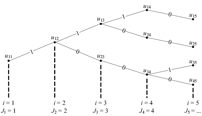
III-A Definitions
With the help of Fig. 1, we give the definitions of path spectrum, population, time spectrum, and expansion factor in turn as follows.
Path Spectrum: When decoding along path , the PDF of is called the path spectrum of along path .
For example, in Fig. 1, there are four decoding paths, each of which corresponds to its path spectrum. Specially, we are interested in the path spectrum along the proper decoding path , which is denoted by , where . According to [19], should satisfy the following constraints
| (6) |
As for the calculation of , three approximation methods have been proposed in [20].
Population: The number of paths after decoding the -th symbol is called the population at time , which is denoted by .
As there is only one path before decoding the first symbol, we have . As for the example of population, please refer to Fig. 1.
Time Spectrum: When decoding the -th symbol, there are paths. We call the PDF of as the time spectrum of at time , which is denoted by .
Please refer to Fig. 1 for the example of time spectrum. As is the PDF of , the normalization property should hold, i.e.
| (7) |
In addition, as we are investigating equiprobable binary sources, the symmetry property should also hold, i.e.
| (8) |
When decoding the first symbol, there is only one path, which is undoubtedly the proper path. Hence, from the statistical view, the time spectrum at time is equivalent to the path spectrum along the proper decoding path , i.e.
| (9) |
Expansion Factor: We define the expansion factor at time as the ratio of the expectation of to that of , which is denoted by , i.e. .
Please refer to Fig. 1 for the example of expansion factor.
III-B Relations between Population, Expansion Factor, and Time Spectrum
When falls into , two branches will be created, or in other word, one more path will be created. Therefore, if there are paths at time , then from the statistical view, more paths will be created at time on average, i.e.
| (10) |
Therefore, the expansion factor at time is
| (11) |
Especially, as and , we have
| (12) |
Then recursively, we have
| (13) |
From the above analyses, we can see that time spectrum is the key to answering all questions. Once we know , expansion factor can be obtained and then population can be deduced in turn.
IV Time Spectrum
IV-A Evolution

With the help of Fig. 2, we illustrate how the time spectrum evolutes as the decoding proceeds. Let be the time spectrum at time . If , then the 0-branch will be created and interval at time will be mapped onto interval at time . It means that the part of over interval will be mapped onto over interval at the next iteration [Fig. 2]. Similarly, if , then the 1-branch will be created and interval at time will be mapped onto interval at time . Meanwhile, the part of over interval will be mapped onto over interval at the next iteration [Fig. 2]. Finally, the time spectrum at time should be the sum of and [Fig. 2], i.e.
| (14) |
where is introduced to make sure . It is easy to obtain
| (15) |
As approaches to the infinite, we have
| (16) |
Hence,
| (17) |
It means: as the decoding proceeds, the time spectrum will converge to the uniform distribution. Meanwhile, we can also obtain . Finally
| (18) |
IV-B Discussion
Intuitively, reflects the residual uncertainty of given its DAC codeword . Therefore, the conditional entropy of given can be calculated by
| (19) |
According to (13), we have
| (20) |
Thus,
| (21) |
It is obvious that
| (22) |
i.e.
| (23) |
Thus, we obtain
| (24) |
Since is the codeword of , the mutual information between and is just the partial information of provided . Recall that the rate of is , so
| (25) |
It means that the rate of a DAC codeword can reach the mutual information between it and the coded source, or in other word, any rate- DAC codeword conveys bits information of the coded source on average.
IV-C Numeric Approximation
As path spectrum , to find the closed form of time spectrum is not an easy thing. Thus, inspired by the work in [20], the author proposes a numeric method for calculating . This method is described in detail below.
IV-C1 Discretization
We divide the interval into uniform cells. Let . Then can be approximated by , where , for a large .
IV-C2 Initialization
Before iteration, we set , , where can be obtained by the method given in [20].
IV-C3 Update
Recursively, can be obtained from by (we omit coefficient )
| (26) |
IV-C4 Normalization
As , we have , i.e.
| (27) |
Let , then should be normalized as
| (28) |
IV-C5 Expansion Factor
Let and , then the expansion factor at time can be calculated by
| (29) |
V Simulation Results

Fig. 3 includes some theoretical and experimental results of expansion factor. For theoretical results, the author first calculates the path spectrum along the proper decoding path through the numeric method given in [20], where the number of cells is set to . Then seeded with , the numeric method given in Section IV-C is run to obtain , where the number of cells is also set to . Finally, the expansion factor at time is obtained by (29).
For experimental results, a 31-bit DAC codec is used to encode various length-1024 equiprobable binary sequences. Then these codewords are decoded. The decoder first counts the number of length- paths (i.e. only symbols are decoded for each path), , through full search. Then the expansion factor at time can be obtained by , where means the average of over DAC codewords.
From Fig. 3, the reader can find that the theoretical results coincide with the experimental results perfectly. Both theoretical and experimental curves converge to rapidly, meaning that the above analyses are well verified.
VI Conclusion
This paper researches an important problem: how many paths will be created as the DAC decoding proceeds? To answer this question, the author inctroduces the concepts of path spectrum, time spectrum, and expansion factor. The relations between time spectrum, path spectrum, and expansion factor are revealed. A numeric method to calculate time spectrum is proposed. The given experimental and theoretical results coincide with each other perfectly. In the future, the author will continue the work and research another important problem: how about the PDF of the Hamming distances between decoding paths and the source?
References
- [1] J. J. Rissanen, “Generalized Kraft inequality and arithmetic coding,” IBM J. Research and Development, vol. 20, no. 3, pp. 198–203, May 1976.
- [2] P. G. Howard and J. S. Vitter, “Practical implementations of arithmetic coding,” in: Image and Text Compression, pp. 85–112, Kluwer Academic, Norwell, Mass, USA, 1992.
- [3] C. Boyd, J. G. Cleary, S. A. Irvine, I. Rinsma-Melchert, and I. H. Witten, “Integrating error detection into arithmetic coding,” IEEE Trans. Commun., vol. 45, no. 1, pp. 1–3, Jan. 1997.
- [4] B. D. Pettijohn, M. W. Hoffman, and K. Sayood, “Joint source/channel coding using arithmetic codes”, IEEE Trans. Commun., vol. 49, no. 5, pp. 826–836, May 2001.
- [5] T. Guionnet and C. Guillemot, “Soft decoding and synchronization of arithmetic codes: application to image transmission over noisy channels,” IEEE Trans. Image Process., vol. 12, no. 12, pp. 1599–1609, Dec. 2003.
- [6] M. Grangetto, E. Magli, and G. Olmo, “Robust video transmission over error-prone channels via error correcting arithmetic codes,” IEEE Commun. Lett., vol. 7, no. 12, pp. 596–598, Dec. 2003.
- [7] M. Grangetto, E. Magli, and G. Olmo, “A syntax preserving error resilience tool for JPEG2000 based on error correcting arithmetic coding,” IEEE Trans. Image Process., vol. 15, no. 4, pp. 807–818, Apr. 2006.
- [8] M. Grangetto, B. Scanavino, G. Olmo, and S. Bendetto, “Iterative decoding of serially concatenated arithmetic and channel codes with JPEG2000 applications,” IEEE Trans. Image Process., vol. 16, no. 6, pp. 1557–1567, Jun. 2007.
- [9] I. Sodagar, B. B. Chai, and J. Wus, “A new error resilience technique for image compression using arithmetic coding,” in: Proc. IEEE ICASSP, pp. 2127–2130, Istanbul, Turkey, June 2000.
- [10] D. Slepian and J. K. Wolf, “Noiseless coding of correlated information sources,” IEEE Trans. Inf. Theory, vol. 19, no. 4, pp. 471–480, July 1973.
- [11] M. Grangetto, E. Magli, and G. Olmo, “Distributed arithmetic coding,” IEEE Commun. Lett., vol. 11, no. 11, pp. 883–885, Nov. 2007.
- [12] M. Grangetto, E. Magli, and G. Olmo, “Distributed arithmetic coding for the Slepian-Wolf problem,” IEEE Trans. Signal Process., vol. 57, no. 6, pp. 2245–2257, Jun. 2009.
- [13] X. Artigas, S. Malinowski, C. Guillemot, and L. Torres, “Overlapped quasi-arithmetic codes for distributed video coding,” in: Proc. IEEE ICIP, 2007, vol. II, pp. 9–12.
- [14] S. Malinowski, X. Artigas, C. Guillemot, and L. Torres, “Distributed coding using punctured quasi-arithmetic codes for memory and memoryless sources,” IEEE Trans. Signal Process., vol. 57, no. 10, pp. 4154–4158, Oct. 2009.
- [15] M. Grangetto, E. Magli, and G. Olmo, “Symmetric distributed arithmetic coding of correlated sources,” in: Proc. IEEE MMSP, 2007, pp. 111–114.
- [16] M. Grangetto, E. Magli, R. Tron, and G. Olmo, “Rate-compatible distributed arithmetic coding,” IEEE Commun. Lett., vol. 12, no. 8, pp. 575–577, Aug. 2008.
- [17] M. Grangetto, E. Magli, and G. Olmo, “Decoder-driven adaptive distributed arithmetic coding,” in: Proc. IEEE ICIP, 2008, pp. 1128–1131.
- [18] M. Grangetto, E. Magli, and G. Olmo, “Distributed joint source-channel arithmetic coding,” IEEE ICIP, 2010, to be presented, available online: http://www.di.unito.it/~mgrange/
- [19] Y. Fang, “Distribution of distributed arithmetic codewords for equiprobable binary sources,” IEEE Signal Process. Lett., vol. 16, no. 12, pp. 1079–1082, Dec. 2009.
- [20] Y. Fang, “Approximation of DAC codeword distribution for equiprobable binary sources along proper decoding path,” IEEE Trans. Inf. Theory, submitted, available online: http://arxiv.org/abs/1009.5257v1.