Berezinskii-Kosterlitz-Thouless-like percolation transitions in the two-dimensional XY model
Abstract
We study a percolation problem on a substrate formed by two-dimensional XY spin configurations, using Monte Carlo methods. For a given spin configuration we construct percolation clusters by randomly choosing a direction in the spin vector space, and then placing a percolation bond between nearest-neighbor sites and with probability , where governs the percolation process. A line of percolation thresholds is found in the low-temperature range , where is the XY coupling strength. Analysis of the correlation function , defined as the probability that two sites separated by a distance belong to the same percolation cluster, yields algebraic decay for , and the associated critical exponent depends on and . Along the threshold line , the scaling dimension for is, within numerical uncertainties, equal to . On this basis, we conjecture that the percolation transition along the line is of the Berezinskii-Kosterlitz-Thouless type.
pacs
05.50.+q(lattice theory and statistics), 64.60.ah(percolation), 64.60.F-(equilibrium properties near critical points, critical exponents), 75.10.Hk(classical spin models)I Introduction
The XY model is formulated in terms of two-dimensional spins normalized as , residing on the sites of a lattice. The reduced Hamiltonian of the XY model (already divided by with the Boltzmann constant and the temperature) reads
| (1) |
where the sum is over all nearest-neighbor pairs, and is the ferromagnetic coupling strength. The spins are labeled by their site numbers.
It is known from the Mermin-Wagner-Hohenberg-Coleman theorem [1] that there cannot exist spontaneous long-range order as long as is finite in Eq. (1), because thermal fluctuations are strong enough to destroy the order. Nevertheless, the system undergoes a phase transition [2, 3, 4] as the coupling strength increases. This type of transition is of infinite order and is known as the Berezinskii-Kosterlitz-Thouless (BKT) transition. For , the spin-spin correlation function decays exponentially, and the spins form a plasma of vortices; but for , the spin-spin correlation function decays algebraically with an exponent depending on , and the spin configurations contain bound vortex-antivortex pairs. Transitions of the BKT type occur in various kinds of systems. The XY-type of transition is related by duality to roughening transitions in solid-on-solid and related models [5]. Apart from the XY model, BKT transitions are found, among others, in vertex models [6], models of crystal surfaces [7], the antiferromagnetic triangular Ising model [8], string theory [9], network systems [10], superfluid systems [11], and superconducting systems [12]. These models may involve long-range or short-range interactions.
It is also known that certain observables of statistical models are equivalent or closely related to properly defined geometric quantities. For instance, the Potts model can be exactly mapped onto the random-cluster model [13], and the susceptibility of the former is related to the cluster-size distribution of the latter; a similar situation applies to the Nienhuis O() loop model [14] and the equivalent spin model [15]. The Mott-to-superfluid transition in the Bose-Hubbard model can be characterized by the winding number of the world lines of the particles [16]. The geometric percolation [17] process has been employed to study percolation on critical substrates, such as the Ising model [18, 19, 20], the Potts model [21], the O() model [22] and even quantum Hall systems [23].
In this work, we study the percolation problem on the substrate of the XY model (1). There is still some freedom in the choice of the percolation criterion. For instance, one may place percolation bonds between all neighboring XY spins if their orientations differ less than a given angle called the “conducting angle”. This problem was recently investigated by Wang et al. [24]. Here we use a different criterion. For a given spin configuration, we choose a randomly oriented Cartesian reference frame in the two-dimensional spin space, and place bonds between nearest-neighbor pairs, say sites and , with a probability
| (2) |
where parametrizes the percolation problem. Note that for these percolation clusters reduce to those formed by the cluster simulation process of the XY model as described in Sec. II.
The rest of this work is organized as follows. Section III presents our numerical results for the critical points of the XY model on the square as well as on the triangular lattice. Section IV describes the analysis of the percolation problem for both lattices, with an emphasis on the determination of the universal character of this type of percolation transition. We conclude with a discussion in Sec. V.
II Algorithm and Sampled Quantities
II.1 Spin updating algorithm
We employ efficient Monte Carlo simulations of the XY model (1) by means of a cluster method [25, 26]. We use a full cluster decomposition [25] as follows:
- 1.
Choose a randomly oriented Cartesian frame of reference () in the spin space, and project the spin along the and axes as . Accordingly, the scalar product in Eq. (1) is written , so that the Hamiltonian separates into two parts as , with and similar for .
- 2.
Between each pair of nearest-neighboring sites, e.g., site and , place a bond with probability .
- 3.
Construct clusters on the basis of the occupied bonds.
- 4.
Independently for each cluster, flip the components of all the spins in the cluster with probability .
II.2 Sampled quantities
We sampled several quantities, including the second and the fourth moments of the magnetization density, and . These quantities determine the dimensionless Binder ratio [27] as
| (3) |
where is the volume. The susceptibility is .
Denoting the size of the th cluster by , we also sampled the second and the fourth moments of the cluster size distribution as
| (4) |
Accordingly, we define another dimensionless ratio as
| (5) |
Note that for the Ising model in Eq. (5) is equal to in Eq. (3).
Also the spin-spin correlation over distances and was sampled. A third dimensionless ratio is defined as
| (6) |
In the high-temperature range , the spin-spin correlation decays exponentially, and goes to 0 as . At criticality, however, tends to algebraic decay as , and converges to a nontrivial universal value. In an ordered state with a non-zero magnetization density, would converge to 1 instead.
Finally, we define the correlation function as the probability that two sites at a distance belong to the same cluster. We sampled over distances and . The associated dimensionless ratio is defined as
| (7) |
III Critical points
III.1 Square lattice
We simulated the XY model on square lattices with periodic boundary conditions, with system sizes in the range . As usual in Monte Carlo studies, the location of a critical point can well be determined using a dimensionless ratio. This is shown in Fig. 1 for the Binder ratio . For , approaches the infinite-temperature value as , as expected for a normal distribution of the and components of the magnetization. For , rapidly converges to a temperature-dependent value, as expected in the low-temperature XY phase.

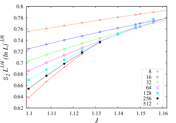
Making use of the known magnetic scaling dimension [4] at the BKT transition, and the logarithmic correction factor with exponent [4, 28], we expect that the scaled quantity tends to a constant at the transition point. The intersections in Fig. 2, which shows this scaled quantity as a function of for several system sizes, confirm this expectation.
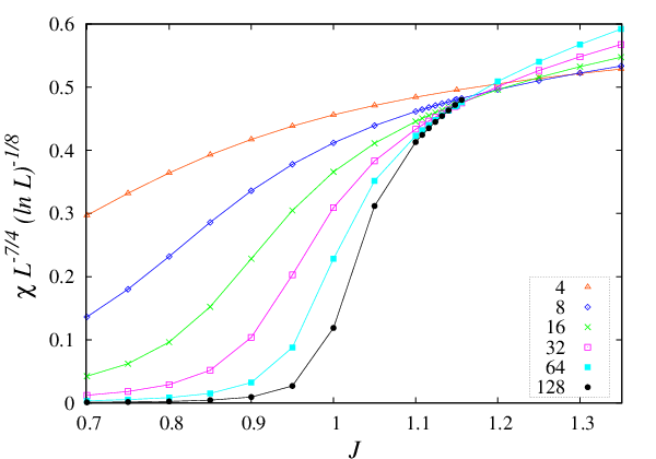

Using the least-squares criterion, we fitted the quantity data by the formula
| (8) | |||||
where the multiplicative and additive logarithmic corrections have been taken into account. We find that the data for and are well described by Eq. (8). The fit yields .
For the Ising model, one can prove that , which exactly relates the thermodynamic quantity to the geometric quantity . We thus expect that, in the case of the XY model, the singularity of coincides with that of . The data for (shown in Fig. 3) were fitted by Eq. (8). This fit yields , consistent with the result from .
III.2 Triangular lattice
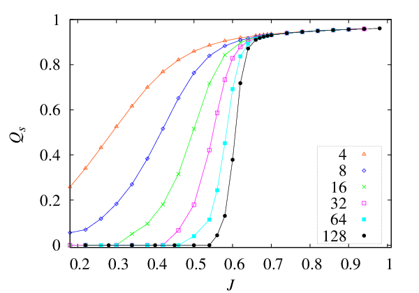
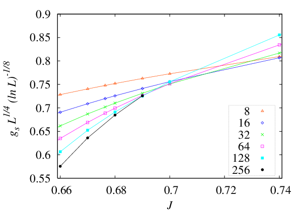
We also simulated the XY model on the triangular lattice with periodic boundary conditions, for linear system sizes in the range . The BKT phase transition is clearly exposed by Fig. 5, which plots the ratio versus the coupling strength . In the high-temperature range , rapidly approaches zero, which reflects the absence of long-range correlations; in the low-temperature range , it converges to a -dependent value smaller than 1, in agreement with the presence of algebraically decaying correlations and the absence of a spontaneous magnetization.
The data near criticality are shown in Fig. 5. They were fitted by Eq. (8), which yielded . Analogous analyses were performed for the scaled susceptibility , leading to . Our results for the critical coupling are consistent with the latest result by Butera and Pernici [30].
IV Percolation analysis
For each spin configuration generated by the Monte Carlo algorithm, we performed a full decomposition in percolation clusters, using the randomly oriented Cartesian frame in the spin space as chosen in the preceding Monte Carlo step, and then placing bonds between nearest-neighbor pairs with probabilities . The variable parameter governs the percolation process. While these percolation clusters are not involved in spin-updating, they reduce to those obtained during the cluster simulations in the case . To analyze this percolation problem, we sampled several quantities, including the second and fourth moments and of the cluster size distribution, the Binder ratio , the correlations , , and the ratio . In this Section we describe the numerical results and analyses, and also an exact result for the present percolation problem on the triangular lattice.
IV.1 Percolation on the square lattice
IV.1.1 High-temperature range
For , i.e. in the limit , all pairs of nearest-neighbor spins are connected as long as their components are pointing in the same direction. At zero coupling , spins at different sites are uncorrelated, so that the percolation process reduces to standard site-percolation process, since the site occupation probability may be identified with the sign of . An unimportant difference is that the present process forms percolation clusters for all the lattice sites while the standard site percolation constructs clusters only for the occupied sites. The site-percolation threshold on the square lattice is very close to 0.592746 [32, 33, 34], and thus no infinite percolation cluster can occur at zero coupling strength , even for . Furthermore, from the results in Ref. [21], where a similar percolation problem is studied in the context of several Potts models, we expect that no percolation transition occurs on the square lattice for small . This expectation was confirmed by Monte Carlo simulations that were performed at several nonzero . Variation of did not yield any signs of a percolation threshold.
IV.1.2 Low-temperature range
The low-temperature XY phase displays algebraically decaying spin-spin correlations, which, unlike the exponential decay at , allows the formation of a divergent percolation cluster for sufficiently large . We may thus expect a percolation threshold to occur at a -dependent value .
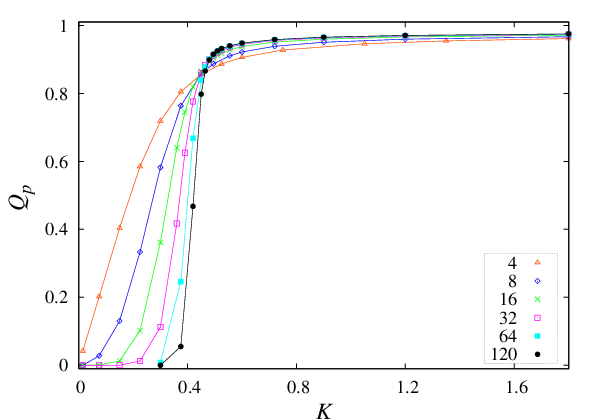

The existence of a percolation threshold for is shown by the intersections of the curves in Fig. 6, which displays as a function of at for several . These data show that . For , rapidly approaches zero, as expected from the absence of long-range correlations of .
In view of the long-range spin-spin correlations for , we have no reason to expect that the percolation transition at the threshold for belongs to the uncorrelated percolation universality class. This is supported by the observation that, at , the fractal dimension of clusters with is , which is different from the value 91/48 for critical percolation clusters [35]. A closer look at the plot of vs. (Fig. 6) indicates that, for , rapidly converges to a -dependent nontrivial value smaller than 1. We propose the interpretation that, like the thermal transition induced by the variation of , the percolation transition induced by is also BKT-like.
In Fig. 7 we display the correlation over a distance as a function of the linear system size for several values of . This figure shows a dependence of on that approaches power-law behavior for large . This suggests that percolation clusters remain critical for . Furthermore the exponent governing the scaling of appears to depend on .
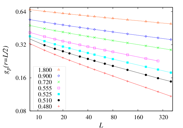


Next, we fitted the data at by
| (9) |
where is the associated scaling dimension. The terms with and describe the finite-size corrections, and the correction exponents are simply set at and , respectively. The results are shown in Table 1.
We conjecture that the fractal dimension of the percolation clusters at assumes the exact BKT value with . This conjecture is based on the BKT-like behavior of the percolation transition in the low-temperature range, and on the numerical evidence for obtained from the correlation in Table 1. First, the percolation in the low-temperature range seems to be BKT-like. Second, the fit results for the scaling dimension , when interpolated to as given in Table 2, yield a value close to . The data for the scaled quantity , shown in Fig. 8 for , confirm the existence of intersections, apparently converging to the same value of as those in Fig. 6. Furthermore we found that the data for in the interval at are well described by Eq. (8) for finite sizes in the range . This fit yields an estimate for the percolation threshold at .
| square | |||||||
|---|---|---|---|---|---|---|---|
| triangular | |||||||
We also performed simulations at , , , and , and observe a behavior similar as that described above for . On the basis of a fit of the data by Eq. (8), we obtain the associated percolation thresholds, which are shown in Table 2. Next, we fitted Eq. (9) to the data at various points for and . The results are shown in Table 3.
In addition, we carried out simulations at , very close to the thermal critical point . The ratio appears to behave similarly as in Fig. 6, which suggests a BKT-like percolation transition. The estimated threshold agrees with the critical point . This fits well with the continuation of the line in Fig. 9. Further, the numerical result for the fractal dimension of the percolation clusters at is consistent with the BKT value .
IV.2 Percolation on the triangular lattice
IV.2.1 Matching property
The matching property [36, 37] plays an important role in the determination of the site percolation thresholds of several two-dimensional lattices; here we briefly review this subject. For a given planar lattice , where is the set of lattice sites and is the edge set, one does the following: 1), select parts of the faces of , and fill in all the “diagonals” in those faces. This yields lattice , where represents the set of all added diagonal edges. 2), select the faces that are not picked up in step 1), and fill in all the diagonals in these faces. One has lattice then with the set of diagonals drawn in step 2). One calls lattices and are matching to each other; note that and may be non-planar. Since no “diagonal” can be filled in a triangle, the triangular lattice is self-matching. It can be shown that, for the site-percolation problem, the cluster numbers per site and on a pair of matching lattices and satisfy
| (10) |
where is the site-occupation probability and is a finite polynomial (it is termed “matching polynomial”). Equation (10) indicates that, if the cluster-number density on the lattice exhibits a singularity at a site occupation probability , the same singularity will also occur in on at . Together with the plausible assumption that there is only one transition, the matching argument yields that the percolation threshold is for all self-matching lattices like the triangular lattice; further, it requires that , which is indeed satisfied by the result [37] for self-matching lattices. An important feature of the matching argument is that it is still valid in the presence of interactions, as long as these interactions are symmetrical under the interchange of occupied and unoccupied sites.
IV.2.2 Percolation at
As mentioned in Sec. IV.1.1, the case , in the present percolation process corresponds with the case for the standard-site percolation. The standard site-percolation threshold for the triangular lattice is , thus the percolation threshold of the present percolation problem at is .
Since the matching argument is independent of the coupling , and no spontaneous symmetry breaking occurs in the two-dimensional XY model, describes a critical line for finite . Further, we expect that, in the high-temperature range , the percolation transition is in the universality class of standard uncorrelated percolation, since there is no long-range spin-spin correlation.
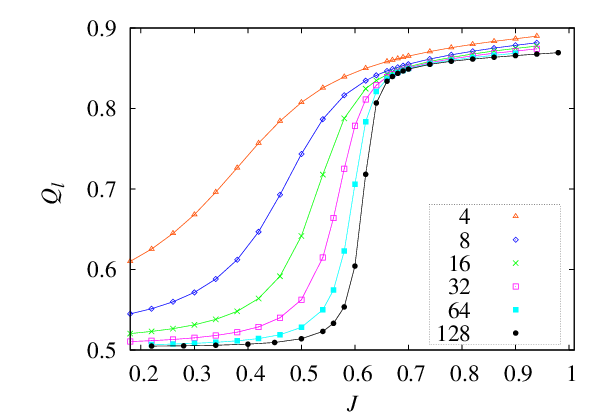
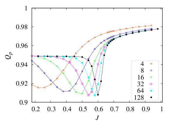
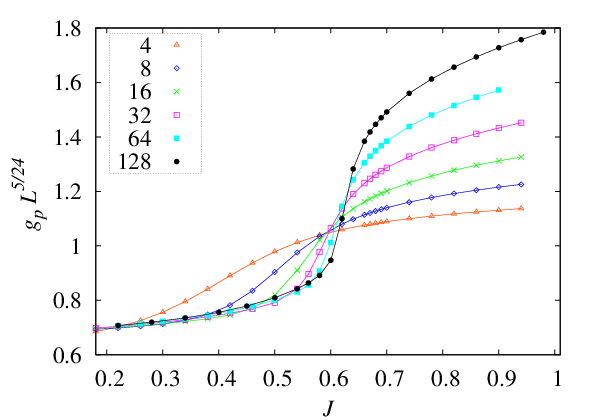
Figure 13 shows the data for the ratio , which is defined by Eq. (5) on the basis of the size distributions of the percolation clusters. For , approaches a -dependent value which is clearly smaller than 1. This implies the absence of an infinite cluster that occupies a finite fraction of the whole lattice. The singularity at the thermal transition point is reflected by the jump that develops near .
Figure 13 shows the data for the ratio . For , converges to a universal value (note that this value differs from [38] for standard percolation on the triangular lattice, due to the difference mentioned in the first paragraph of Sec. IV.1.1). For , approaches a -dependent value smaller than 1; we thus expect that the correlation decays algebraically rather than exponentially. The thermal transition at is reflected by the rapid variation of near for large .
The data for the scaled correlation at are shown in Fig. 13 as a function of , with for the uncorrelated percolation universality. The convergent behavior for as a function of confirms that the transition in this range belongs to the standard percolation universality class. The intersections roughly represent the thermal transition point .
IV.2.3 Percolation at
Following similar procedures as in Sec. IV.1, we obtain a percolation line in low the temperature range for the triangular lattice. For we do not find a percolation threshold at finite values of . The numerical results are shown in Table 2 and Fig. 14. It is observed that the percolation in the range is also BKT-like, with a fractal dimension at , and a scaling dimension depending on parameters and in the range . This is consistent with the results for the square lattice in Sec. IV.1.

V Discussion
Since spins in the same cluster formed during the simulations must have -components of the same sign, the absence of a spontaneous magnetization [1] in the XY model means that the density of the largest cluster in the thermodynamic limit is also restricted to be zero, at least for finite values of . The same restriction thus applies to percolation clusters formed with in Eq. (2), and it must also hold for . The absence of a nonzero density of the largest percolation cluster is in agreement with the interpretation of the percolation transitions for described in Sec. IV as BKT-like.
The results presented in Sec. IV.1 for the square lattice indicate that, in addition to the line with , also the line , represents a percolation threshold. As can be seen from the data points for in Fig. 10, the magnetic exponent depends on along the latter line, which is thus a “nonuniversal” line of percolation transitions, and the bond dilution field parametrized by is truly marginal. The existence of a BKT transition induced by varying at the point corresponds with a marginally relevant bond-dilution field in the direction.
As mentioned earlier, for the triangular lattice with , the line is critical, and belongs to the standard percolation universality class. The continuation of the line to is also critical (in the sense that the correlation functions display algebraic decay), but with a -dependent critical exponent.
In order to obtain some more information on the dependence of the present percolation problem on the coordination number , we also simulated the equivalent-neighbor XY model on the triangular lattice, which has equal nearest-, second-nearest- and third-nearest-neighbor interactions. The procedure outlined in Sec. (III) yielded an estimate of the thermal transition at . As expected, a Monte Carlo analysis of the percolation problem with showed the existence of a critical line in the high-temperature phase , belonging to the standard percolation universality class. When approaches , the line bends toward large values of . This suggests that line ends at for . For there is clear evidence for the existence of a percolation cluster with a finite density in the limit of large .
In the low-temperature range , we found, just as for the models with nearest-neighbor interactions, a BKT-like transition line , as in Figs. 9 and 14. In spite of the relatively large coordination number , no evidence is found for a percolation cluster of a nonzero density, even at . Although the spin-spin correlations in the algebraic XY phase for stimulate the percolation transition in the sense that it occurs at smaller values of when increases, it also appears that they obstruct the formation of a percolation cluster with a non-zero density.
Besides the rule based on Eq. (2), other procedures for placing bonds may be applied. For instance, as mentioned in the Introduction, Wang et al. [24] placed percolation bonds between neighboring XY spins if their orientations differ less than a given threshold, and found percolation transitions in the uncorrelated percolation universality class for all XY couplings. Another possibility is to place percolation bonds with probabilities given, instead of Eq. (2), by . In that case, we expect percolation transitions similar to those of Ref. 24, including transitions in the low-temperature range of the XY model. Indeed, a preliminary Monte Carlo analysis of this problem [39] confirms the existence of such transitions in the universality class of uncorrelated percolation.
Finally we remark that recently a percolation problem was formulated on the basis of the O() loop configurations [22]. Since the XY model is equivalent with the O(2) model, another way thus arises to introduce percolation in XY-type models. Although this seems a very different approach, it reproduces our result that a marginally relevant dilution field exists at the BKT transition.
Acknowledgements.
We are indebted to Prof. B. Nienhuis for valuable discussions. This work was supported in part by the National Nature Science Foundation of China under Grant No. 10975127, the Anhui Provincial Natural Science Foundation under Grant No. 090416224, and the Chinese Academy of Sciences.References
- [1] N. D. Mermin and H. Wagner, Phys. Rev. Lett. 17, 1133 (1966); N. D. Mermin, J. Math. Phys. 8, 1061 (1967); P. C. Hohenberg, Phys. Rev. 158, 383 (1967); S. Coleman, Commun. Math. Phys. 31, 259 (1973).
- [2] V. L. Berezinskii, Zh. Eksp. Teor. Fiz. 59, 907 (1970) [Sov.Phys. JETP 32, 493 (1971)].
- [3] J. M. Kosterlitz and D. J. Thouless, J. Phys. C 5, L124 (1972); J. Phys. C 6, 1181 (1973).
- [4] J. M. Kosterlitz, J. Phys. C 7, 1046 (1974).
- [5] J. V. José, L. P. Kadanoff, S. Kirkpatrick and D. R. Nelson, Phys. Rev. B 16, 1217 (1977).
- [6] E. H. Lieb and F. Y. Wu, in Phase Transitions and Critical Phenomena, edited by C. Domb and M. S. Green (Academic Press, London, 1972), Vol. 1.
- [7] H. van Beijeren, Phys. Rev. Lett. 38, 993 (1977).
- [8] B. Nienhuis, H. J. Hilhorst and H. W. J. Blöte, J. Phys. A 17, 3559 (1984); X.-F. Qian and H. W. J. Blöte, Phys. Rev. E 70, 036112 (p.1-8) (2004).
- [9] M. Maggiore, Nucl. Phys. B 647, 69 (2002).
- [10] M. Bauer, S. Coulomb, and S. N. Dorogovtsev, Phys. Rev. Lett. 94, 200602 (2005); M. Hinczewski and A. N. Berker, Phys. Rev. E 73, 066126 (2006); E. Khajeh, S. N. Dorogovtsev, and J. F. F. Mendes, Phys. Rev. E 75, 041112 (2007); A. N. Berker, M. Hinczewski, and R. R. Netz, Phys. Rev. E 80, 041118 (2009).
- [11] D. J. Bishop and J. D. Reppy, Phys. Rev. Lett. 40, 1727 (1978).
- [12] D. J. Resnick, J. C. Garland, J. T. Boyd, S. Shoemaker and R. S. Newrock, Phys. Rev. Lett. 47, 1542 (1981).
- [13] P. W. Kasteleyn and C. M. Fortuin, J. Phys. Soc. Jpn. 46 (Suppl.), 11 (1969); C. M. Fortuin and P. W. Kasteleyn, Physica (Amsterdam) 57, 536 (1972).
- [14] B. Nienhuis, Phys. Rev. Lett. 49, 1062 (1982); J. Stat. Phys. 34, 731 (1984).
- [15] E. Domany, D. Mukamel, B. Nienhuis, and A. Schwinger, Nucl. Phys. B 190, 279 (1981).
- [16] E. L. Pollock and D. M. Ceperley, Phys. Rev. B 36, 8343 (1987).
- [17] D. Stauffer and A. Aharony, Introduction to Percolation Theory, Ed. (Taylor and Francis,1994); G. Grimmett, Percolation, Ed. (Springer, 1999).
- [18] M. F. Sykes and D. S. Gaunt, J. Phys. A 9, 2131 (1976).
- [19] A. Coniglio, C. R. Nappi, F. Peruggi, and L. Russo, J. Phys. A 10, 205 (1977).
- [20] Y. Deng and H. W. J. Blöte, Phys. Rev. E 70, 056132 (2004).
- [21] X.-F. Qian, Y. Deng and H. W. J. Blöte, Phys. Rev. B 71, 144303 (2005).
- [22] C.-X. Ding, Y. Deng, W.-A. Guo, and H. W. J. Blöte, Phys. Rev. E 79, 061118 (2009).
- [23] D.-H. Lee, Z. Wang, and S. Kivelson, Phys. Rev. Lett. 70, 4130 (1993).
- [24] Y. Wang, W.-A. Guo, B. Nienhuis and H. W. J. Blöte, Phys. Rev. E 81, 031117 (2010).
- [25] R. H. Swendsen and J. S. Wang, Phys. Rev. Lett. 58, 86 (1987).
- [26] U. Wolff, Phys. Rev. Lett. 60, 1461 (1988).
- [27] K. Binder, Z. Phys. B 43, 119 (1981).
- [28] D. J. Amit, Y. Y. Goldschmidt, and G. Grinstein, J. Phys. A 13, 585 (1980); L. P. Kadanoff and A. B. Zisook, Nucl. Phys. B 180 (FS2), 61 (1981); R. Kenna, Preprint cond-mat/0512356 at arxiv.org (2005).
- [29] M. Hasenbusch and K. Pinn, J. Phys. A 30, 63 (1997); M. Hasenbusch, J. Phys. A 38, 5869 (2005).
- [30] P. Butera and M. Pernici, Physica A 387, 6293 (2008).
- [31] H. Arisue, Phys. Rev. E 79, 011107 (2009).
- [32] M. E. J. Newman and R. M. Ziff, Phys. Rev. Lett. 85, 4104 (2000).
- [33] M. J. Lee, Phys. Rev. E 76, 027702 (2007).
- [34] X. M. Feng, Y. Deng and H. W. J. Blöte, Phys. Rev. E 78, 031136 (2008).
- [35]
B. Nienhuis, in Phase Transitions and Critical Phenomena, edited by C. Domb
and J. L. Lebowitz (Academic Press, London, 1987), Vol. 11;
J. L. Cardy, in Phase Transitions and Critical Phenomena, edited by C. Domb and J. L. Lebowitz (Academic Press, London, 1987), Vol. 11. - [36] M. F. Sykes and J. W. Essam, J. Math. Phys. 5, 1117 (1964).
- [37] J. M. Essam, in Phase Transitions and Critical Phenomena, edited by C. Domb and M. S. Green (Academic Press, London, 1987), Vol. 2, p.197.
- [38] W. Zhang and Y. Deng, Wrapping probabilities and percolation thresholds in two and three dimensions, in preparation (2010).
- [39] H. Hu and Y. Deng, unpublished results (2010).