New proofs of certain finite filling results via Khovanov homologyThanks: Partially supported by an NSERC postdoctoral fellowship.
Abstract.
We give a Khovanov homology proof that hyperbolic twist knots do not admit non-trivial Dehn surgeries with finite fundamental group.
1. Introduction
Twists knots provide the simplest infinite family of hyperbolic knots. These arise by considering various twisted Whitehead doubles of the trivial knot, for example. Alternatively, and better suited to the purpose of this paper, let be the -pretzel knot and consider the family where (see Figure 1). With this convention, is the left-handed trefoil knot and is the figure eight knot. For the knot is hyperbolic.
 \labellist\pinlabel at 488 440
\endlabellist
\labellist\pinlabel at 488 440
\endlabellist
Given a knot in , consider the three-manifold with torus boundary where is an open tubular neighbourhood of the knot. Define where is the homeomorphism determined by . In this notation, is the knot meridian, is the Seifert longitude, and is an extended reduced rational number. The resulting closed three-manifold is the result of -surgery on ; notice that the trivial surgery corresponds to the extended rational . For background consistent with these conventions we refer the reader to Boyer [3].
A non-trivial surgery with finite fundamental group is called a finite filling. These fillings give a special type of exceptional surgery on a hyperbolic knot; a result of Thurston states that hyperbolic knots admit finitely many exceptional surgeries [16, 17]. The aim of this paper is to use Khovanov homology to prove the following:
This result was first proved by Delman using essential laminations [7], and independently by Tanguay via character variety methods [15]. A complete classification of exceptional surgeries on two-bridge knots was subsequently obtained by Brittenham and Wu [6]. Note also that Boyer, Mattman and Zhang give a complete description of the fundamental polygon of any twist knot, from which Tanguay’s proof may be recovered [4].
An alternate proof of Theorem 1.1 may be obtained via Heegaard Floer homology. Since twist knots are alternating, it follows that hyperbolic twist knots do not admit L-space surgeries [13, Theorem 1.5]. As manifolds with elliptic geometry are L-spaces [13, Proposition 2.3], Theorem 1.1 follows. This appeals to an equivalence between manifolds with finite fundamental group and manifolds admitting elliptic geometry, though in the present setting geometrization in full generality is not required; the presence of a strong inversion (as described below) ensures that geometrization for orbifolds of cyclic type is sufficient [2, 17].
A strong inversion is an involution of a three-manifold with one-dimensional fixed point set. For example, every two-fold branched cover of admits a strong inversion. A knot in is strongly invertible if the standard strong inversion on induces a strong inversion on the knot complement . That is, admits an involution with one-dimensional fixed point set meeting transversally in exactly 4 points. The twist knot is strongly invertible for all ; the relevant symmetry is exhibited in Figure 1.
Given a strongly invertible knot, the involution on the knot complement may be extended to a strong inversion on any surgery [12]. This is referred to as the Montesinos trick, and as a result every surgery on a strongly invertible knot may be realized as a two-fold branched cover of branched over a link. In this setting, the work in [20] establishes that Khovanov homology may be used to provide obstructions to finite fillings. This makes use of the Khovanov homology of the branch sets associated with a surgery on the knot via Montesinos’ work. For example, Khovanov homology easily recovers the fact that the figure eight knot does not admit finite fillings [20, Theorem 7.2] (this result is originally due to Thurston [16]). The key observation is that, to a certain degree, relatively simple two-fold branched covers (in terms of geometry) have branch sets with simple Khovanov homology.
Using the strong inversion on , the goal of this paper is to apply the results in [20] to prove Theorem 1.1. The proof is entirely combinatorial and new, in the sense that it does not appeal to any of the machinery described above (Heegaard Floer homology, character varieties, essential laminations, etc.). However, the relationship between Heegaard Floer homology and Khovanov homology suggests that the particular obstructions from these two theories may be related. Part of the motivation for pursuing a proof via Khovanov homology stems from an interest in comparing the obstructions from Heegaard Floer homology and from Khovanov homology. Further motivation is in establishing methods for applying obstructions from Khovanov homology to infinite families. This poses the immediate challenge of pushing calculation techniques beyond the limits imposed by machine calculation, and in turn is a central focus of this paper.
1.1. The proof of Theorem 1.1
The feature of Khovanov homology exploited in this proof is homological width. For a given link this is the integer recording the number of diagonals supporting non-trivial homology (see Definition 3.1). Let denote the two-fold branched cover of branched over a link . The following is proved in [20]:
Theorem 1.2 ([20, Theorem 6.3]).
If has finite fundamental group then .
With this result in hand the aim of this paper is to establish:
Theorem 1.3.
The surgery may be realized as the two-fold branched cover , where the branch set satisfies .
When , Theorem 1.1 follows immediately from Theorem 1.2 and Theorem 1.3. The case corresponds to surgery on the figure eight knot and we appeal to the amphichirality of combined with the fact that the width bound of Theorem 1.2 for finite fillings is violated for non-negative surgery coefficients (compare [20, Theorem 7.2]).
The remainder of the paper is devoted to establishing Theorem 1.3, and is organized as follows. The proof has essentially two parts: first describe the exterior of each as the two-fold branched cover of a tangle (see Proposition 2.1), and second determine the coarse behaviour of the Khovanov homology (precisely, the homological width) of various rational closures of these tangles (see Proposition 4.2). The former is established in Section 2 and is a straightforward application of the Montesinos trick, while calculations pertaining to the latter occupy Section 4.
A key observation is that relatively few integer surgeries need to be considered in order to infer the homological width for the infinite family of branch sets associated with each knot . This exploits some particularly stable behaviour of the families of links that arise, as developed in [20]. The sense in which the homological width might be considered coarse information is elucidated through these calculations. Indeed, we will only calculate the Khovanov homology for certain branch sets up to indeterminate summands (see Remark 3.4), thus the homological width is obtained without a full description of the Khovanov homology. Since Khovanov homology can be difficult to compute for knots with a high number of crossings, this suggests that it may be possible to calculate (or bound) the homological width in certain settings without needing to calculate the entire invariant.
For the reader’s reference, we have collected the requisite properties of reduced Khovanov homology with coefficients in in Section 3. This section constitutes the bulk of the paper, and may be skipped at first reading by those already familiar with the invariant.
Acknowledgements
Much of the work associated with this paper was completed while in residence at MSRI in 2010. The author thanks the organizers of the program Homology Theories of Knots and Links for providing a stimulating work environment. Thanks also to Tye Lidman for helpful discussions pertaining to spectral sequences, Paul Turner for comments on an earlier draft of this paper, and Jeremy Van Horn-Morris for valuable comments regarding open book decompositions. Finally, the detailed comments provided by the referees improved the exposition of the paper throughout.
2. Branch sets
Given a manifold obtained by Dehn surgery on a strongly invertible knot, the Montesinos trick provides an alternate description of the manifold as a two-fold branched cover of [12]. To make this precise we review the notation introduced in [20, Section 3]. When is strongly invertible, the knot exterior is the two-fold branched cover of a tangle where is a three-ball and is a pair of properly embedded arcs. Denote this two-fold branched cover by . The arcs are the image of the fixed point set in the quotient of the involution on the exterior . As a result, the tangle is well-defined up to homeomorphism of the pair , and any diagram of may be regarded as a choice of representative for the homeomorphism class.
The boundary of the knot exterior has a preferred generating set for homology given by the knot meridian and the Seifert longitude . It is always possible to make a choice of corresponding preferred representative for the homeomorphism class of the pair as illustrated in Figure 2 (see [20, Corollary 3.8], for example). That is, and provide explicit descriptions of the branch sets corresponding to the trivial and zero surgeries, respectively. This may be thought of as fixing a framing on the tangle , just as corresponds to the Seifert framing of the knot. Throughout this paper we will use to denote the preferred representative of the associated quotient tangle of a given strongly invertible knot.
at -80 278 \pinlabel at -150 210 \pinlabel at 280 210 \pinlabel at 620 210 \endlabellist
More generally, branch sets for the integer surgeries are given by the links as in Figure 3 so that . In particular, notice that the half twist in the branch set lifts to a full Dehn twist in the cover, so that is the branch set for the manifold obtained by filling along the slope in the boundary of the knot exterior. It follows that (recall that whenever is finite, and zero otherwise). It is also possible to describe -surgery on a strongly invertible knot (having fixed a continued fraction expansion of the surgery coefficient) so that ; see [20, Section 3] for details.
at 382 464
\pinlabel at 325 395
\endlabellist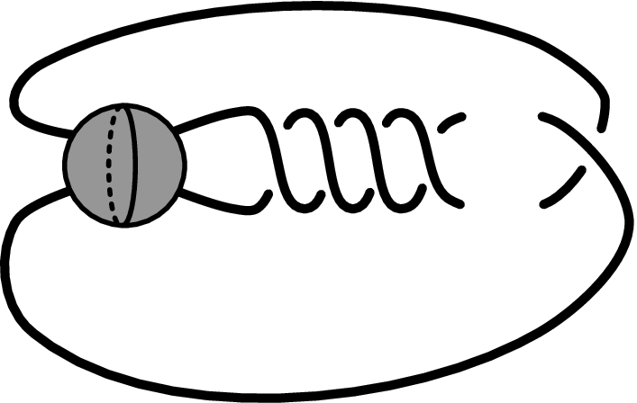 \labellist\pinlabel at 351 380
\endlabellist
\labellist\pinlabel at 351 380
\endlabellist
The goal of this section is to determine the tangle associated with the strong inversion on the twist knot illustrated in Figure 1; this will establish the first part of Theorem 1.3. As a first approximation, we determine the tangle associated with the quotient of , without keeping track of the preferred representative (as described above) corresponding to the pair . This quotient is described in Figure 4 and is simplified in Figure 5.
at 193 293
\pinlabel at 773 285
\pinlabel
at 865 340
\pinlabel at 925 340
\endlabellist
at 308 458 \pinlabel at 170 485 \pinlabel at 110 485 \pinlabel at 368 624 \pinlabel at 368 565 \pinlabel at 368 355 \pinlabel at 368 300 \endlabellist \labellist\pinlabel at 273 511 \pinlabel at 148 500 \pinlabel at 89 500 \pinlabel at 355 615 \pinlabel at 328 590 \pinlabel at 328 385 \pinlabel at 355 374 \endlabellist \labellist\pinlabel at 347 411 \pinlabel at 342 347 \pinlabel at 120 540 \pinlabel at 120 323 \pinlabel at 455 323 \pinlabel at 455 540 \endlabellist
The closure of the tangle diagram in Figure 5 that gives the trivial knot (by joining to and to ) identifies the trivial surgery in the cover, and therefore the preferred representative for this tangle is obtained by adding some collection of horizontal twists. That is, the tangle diagram in Figure 5 describes a representative for the associated quotient tangle that is compatible with some integer framing, but not necessarily the Seifert framing. In particular, the right hand half twist between the strands meeting and lifts to a full Dehn twist along the knot meridian in the two-fold branched cover.
Recall that is a presentation for the three-strand braid group, where braid words are read from left to right. Our convention for the generators is given in Figure 6. Figure 5 suggests that the desired collection of branch sets may be represented by closures of three-strand braids (see Figure 7). From this observation the relevant family of braids to consider is given by , and determining the preferred representative amounts to establishing the appropriate framing, controlled by the integer .
at 375 463
\pinlabel at 95 463
\endlabellist
at 216 142 \pinlabel at 210 82 \endlabellist \labellist\pinlabel at 400 415 \pinlabel at 397 372 \endlabellist
We claim that the branch set is the closure of the braid
where
so that . Note that the non-negative integer determines the twist knot, while the integer is the surgery coefficient.
To see that this is the correct framing, it suffices to verify that , since and lifts to the positive Dehn twist about the meridian. We leave this verification to the reader (for the moment), but note that calculations in Section 4 will provide a proof (see Remark 4.7).
The braid relation establishes that and are equivalent, the latter representing the full twist on three strands. As this element is central in the the braid group, have now shown:
Proposition 2.1.
The branch set is given by the closure of the braid
where .
Remark 2.2.
It is possible to find the preferred representative directly (as in Bleiler [1], for example). This amounts to (carefully) carrying the image of the longitude through the quotient shown in Figure 4 and the subsequent tangle isotopies of Figure 5. In the present setting, the key observation is that a full twist in the cover (taking to ) corresponds to the addition of in the base. One checks that the addition of the full twist in the branch set preserves the Seifert framing in the cover, and as a result it is possible to induct in (in fact, two separate inductions for odd and even) to determine that the preferred representative . The base case may be extracted from [20, Section 3.2] together with the Seifert fibre structure on the trefoil exterior, while the base case may be extracted from [20, Section 7.1].
This calculation sets up our second task towards the proof of Theorem 1.1: determine the reduced Khovanov homology for closures of the family of three-braids . To conclude this discussion, Jeremy Van Horn-Morris points out that realizing the branch set as the closure of a three-strand braid also establishes the following:
Corollary 2.3.
The result of integer Dehn surgery on admits a genus one open book decomposition, for each . Moreover, for positive integer Dehn surgeries the corresponding open book decomposition has positive monodromy.
3. Khovanov homology
3.1. Grading conventions for reduced Khovanov homology
Throughout this work we make use of the reduced Khovanov homology of a link , with coefficients in , denoted [8, 9]. For our purposes, this is a -graded group, with primary (cohomological) grading and secondary (quantum) grading . Note that by setting the Jones polynomial of is given by
In particular, our primary grading is by diagonals of slope 2 in the -plane for the standard bigrading in Khovanov homology [8].
Definition 3.1.
The homological width of a link is the integer determined by the number of -gradings supporting non-trivial homology in .
This grading convention, specifically suited to considerations involving homological width, is consistent with that of Manolescu and Ozsváth [11]. For example, let denote the trivial knot. Then supported in bigrading (with ), while , with one generator supported in each bigrading and (with ). These examples are illustrated in Figure 8.
at 324 413
at 323 378
\pinlabel at 290 413
\endlabellist \labellist\pinlabel at 324 450
\pinlabel at 360 413
\pinlabel at 318 378
\pinlabel at 356 378
\pinlabel at 284 413
\pinlabel at 290 450
\endlabellist \labellist\pinlabel at 324 413
\pinlabel at 324 485 \pinlabel at 321 378
\pinlabel at 290 413
\pinlabel at 290 450
\pinlabel at 290 485
\endlabellist
\labellist\pinlabel at 324 450
\pinlabel at 360 413
\pinlabel at 318 378
\pinlabel at 356 378
\pinlabel at 284 413
\pinlabel at 290 450
\endlabellist \labellist\pinlabel at 324 413
\pinlabel at 324 485 \pinlabel at 321 378
\pinlabel at 290 413
\pinlabel at 290 450
\pinlabel at 290 485
\endlabellist
3.2. The skein exact sequence as a mapping cone
With the above conventions in place, the long exact sequence in Khovanov homology related to the resolution of a positive crossing may be expressed as a mapping cone
| (1) |
where the connecting homomorphism raises the primary grading by one and fixes the secondary grading. The shift in bigrading is defined by
The constant measures the difference in negative crossings for some choice of orientation on the components of the resolution ![[Uncaptioned image]](1010.3051v2/one-in-text.png) that do not inherit an orientation from
that do not inherit an orientation from ![[Uncaptioned image]](1010.3051v2/right-in-text.png) . Notice that when is the closure of a positive braid . These conventions are consistent with those of Rasmussen [14] and of Manolescu and Ozsváth [11].
. Notice that when is the closure of a positive braid . These conventions are consistent with those of Rasmussen [14] and of Manolescu and Ozsváth [11].
3.3. Spectral sequences from iterated mapping cones
There are various settings in which the mapping cone described above may be efficiently iterated to calculate Khovanov homology. For the present purposes, we establish one such situation given a link represented as the closure of a positive braid. To this end, let where is a positive braid, and fix distinguished crossings. Fixing, additionally, an order on the distinguished crossings gives rise to a collection of positive braids obtained by replacing the first crossings with the oriented resolution ![[Uncaptioned image]](1010.3051v2/zero-in-text.png) . Similarly, the link produces a collection of resolutions obtained by replacing the first crossings by the oriented resolution and the with unoriented resolution . (A schematic illustrating the case in an example is shown in Figure 12.) Of course, the are no longer link diagrams in closed-braid form. For each link fix the constant for some choice of orientation on compatible with the orientation on the unaffected components of , as in the previous section. As a result, from the grading shifts in (1) we have that
. Similarly, the link produces a collection of resolutions obtained by replacing the first crossings by the oriented resolution and the with unoriented resolution . (A schematic illustrating the case in an example is shown in Figure 12.) Of course, the are no longer link diagrams in closed-braid form. For each link fix the constant for some choice of orientation on compatible with the orientation on the unaffected components of , as in the previous section. As a result, from the grading shifts in (1) we have that
| (2) |
for , where . Now define
| (3) |
Consulting the definition of , we see that as a bigraded -vector space. Moreover, omitting the internal differentials on the for brevity, the structure of the differential relative to this decomposition is given by
(in the case ) so that, by construction, this decomposition of the chain complex comes with a filtration of the form for . (The differential takes the form in general, where .) As a result, there is an associated spectral sequence with , converging to . We will be most interested in the page of this spectral sequence given by
| (4) |
This notation does not reference the order chosen on the resolved crossings, however the crossings and their order will always be made explicit in applications. Notice that the differential on the page is lower triangular (and filtered by diagonals) if we choose a basis corresponding to
(the grading shifts have been omitted for brevity). In particular, is never in the target of the differential.
While the higher differentials may be difficult to calculate in general, the construction ensures that each of these raises -grading by one and fixes the -grading, as in the case of the mapping cone from which this spectral sequence is derived. (Note that we are ignoring the spectral sequence grading and working with the grading inherited from .) Indeed, this construction in the case gives the two step complex
associated with the mapping cone, as in the previous section.
Even in the case , obtaining the differential essentially amounts to calculating the reduced Khovanov homology directly from the definition. In practice, computing the homology by way of this spectral sequence is tantamount to (careful) iterations of the long exact sequence. However, the page described here can be useful when combined with additional structure (described below). It should be noted that this spectral sequence is closely related to the spectral sequence used by Turner [19] to compute the (unreduced) Khovanov homology of -torus links (with coefficients in ). Indeed, we will revisit this calculation in Section 3.5. However, we reiterate that the set-up here ignores the spectral sequence gradings; we opt instead to use the grading inherited from . Another related instance of this construction is given in [20, Lemma 4.10] (see also Proposition 4.3).
3.4. Turner’s spectral sequence
There is an analogy to Lee’s spectral sequence [10] for reduced Khovanov homology due to Turner [18], summarized as follows:
Theorem 3.2 (Turner [18]).
There is a perturbed version of the reduced Khovanov complex with homology denoted for which . Moreover, there is a spectral sequence converging to , with , satisfying the properties that
(1) the differential on the page is of bi-degree , and
(2) for each
| (5) |
where the denote the components of the link ; therefore is at least this quantity.
Our main computational tool will be in combining the structure of with the iterated the mapping cone. Since these both arise from spectral sequence constructions, we will endeavour to refer to pairings when higher differentials computing are in question, and differentials when referring to the iterated mapping cone in an attempt to avoid confusion.
3.5. The reduced Khovanov homology of a full twist
The reduced Khovanov homology for the first 3 non-trivial torus links on three strands is described in Figure 9. The -grading is read horizontally and the -grading is read vertically. The values at a given lattice point denote the rank of the -vector space in that bigrading; empty lattice points are read as rank zero.
at 324 413 \pinlabel at 324 485 \pinlabel at 324 522
at 321 378
\pinlabel at 290 413
\pinlabel at 290 450
\pinlabel at 290 485
\pinlabel at 290 522
\endlabellist \labellist\pinlabel at 324 413
\pinlabel at 324 485
\pinlabel at 324 522
\pinlabel at 324 557
\labellist\pinlabel at 324 413
\pinlabel at 324 485
\pinlabel at 324 522
\pinlabel at 324 557
at 359 522
at 321 378 \pinlabel at 356 378 \pinlabel at 290 413 \pinlabel at 290 450 \pinlabel at 290 485 \pinlabel at 290 522 \pinlabel at 290 557
\labellist\pinlabel at 324 413 \pinlabel at 324 485 \pinlabel at 324 522 \pinlabel at 324 594
at 359 522
at 321 378
\pinlabel at 356 378
\pinlabel at 290 413
\pinlabel at 290 450
\pinlabel at 290 485
\pinlabel at 290 522
\pinlabel at 290 557
\pinlabel at 290 594
\endlabellist
Using Lee’s spectral sequence, Turner establishes the full Khovanov homology (with coefficients in ) for three-strand torus links [19]. Following this proof, a similar result may be established in the present setting, modulo a particular indeterminate summand described in Figure 10. We will ultimately be interested in the -torus links for . Note that this is the closure of the braid .
\labellist\pinlabel at 324 450 \pinlabel at 324 485
at 360 413 \pinlabel at 360 450 \endlabellist \labellist\pinlabel at 324 485 \pinlabel at 360 413 \endlabellist
Remark 3.4.
Since we will be interested only in coarse properties of the Khovanov homology of the full twist in the sequel (in particular, the homological width), the actual value of this indeterminate summand will have no contribution. In practice, the actual rank of this summand is 2 (as in for example, see Figure 9), though we will not prove this in general. Calculation up to indeterminate summands is relatively easy, and in general the homological width of a link seems easier to determine than the complete Khovanov homology.
Proposition 3.5.
The reduced Khovanov homology of the positive torus link is described in Figure 11 for .
\labellist\pinlabel at 324 413 \pinlabel at 324 485 \pinlabel at 324 522
at 360 594 \pinlabel at 360 630
at 432 702 \pinlabel at 432 739
at 468 810 \pinlabel at 468 846
at 400 671
at 322 363 \pinlabel at 357 363 \pinlabel at 396 365 \pinlabel at 468 363
at 275 413 \pinlabel at 275 450 \pinlabel at 285 495
at 275 810
\pinlabel at 275 845 \endlabellist \labellist\pinlabel at 324 413
\pinlabel at 324 485
\pinlabel at 324 522
\labellist\pinlabel at 324 413
\pinlabel at 324 485
\pinlabel at 324 522
at 360 594 \pinlabel at 360 630
at 432 702 \pinlabel at 432 739
at 468 810 \pinlabel at 468 846
at 468 879
at 504 844
at 400 671
at 322 363 \pinlabel at 357 363 \pinlabel at 396 365 \pinlabel at 503 363
at 275 413 \pinlabel at 285 450 \pinlabel at 285 495
at 275 845 \pinlabel at 285 881
 \labellist\pinlabel at 324 413
\pinlabel at 324 485
\pinlabel at 324 522
\labellist\pinlabel at 324 413
\pinlabel at 324 485
\pinlabel at 324 522
at 360 594 \pinlabel at 360 630
at 432 702 \pinlabel at 432 739
at 468 810 \pinlabel at 468 846
at 525 720 \pinlabel at 550 720 \pinlabel at 400 671
at 322 367 \pinlabel at 357 363 \pinlabel at 396 365 \pinlabel at 505 367
at 285 413 \pinlabel at 275 450 \pinlabel at 285 495
at 275 881 \pinlabel at 275 918
Following Turner [19], the proof of Proposition 3.5 is by induction in (with base case provided by Figure 9) in three steps:
Claim 3.6.
If the result holds for then it holds for .
Claim 3.7.
If the result holds for then it holds for .
Claim 3.8.
If the result holds for then it holds for .
The strategy to prove each claim is identical: for appropriately chosen , iterate the skein exact sequence as summarized in Figure 12 to obtain as described in Section 3.3. In each case this expresses in terms of together with a collection of possible new generators. With these possible new generators in hand, the structure of forces the behaviour of the differentials to give the result in each case.
at 324 413
at 359 484 \pinlabel at 359 522
at 359 557
at 396 522
at 330 370 \pinlabel at 359 375 \pinlabel at 390 365
at 290 530
\pinlabel at 290 557
\endlabellist \labellist\pinlabel at 324 413
at 359 484 \pinlabel at 359 522
at 359 557
at 396 522
at 396 557
at 359 595
at 330 370 \pinlabel at 359 357 \pinlabel at 390 370
at 275 530 \pinlabel at 275 557 \pinlabel at 275 593 \endlabellist \labellist\pinlabel at 324 413
at 359 484 \pinlabel at 359 522
at 395 593 \pinlabel at 395 630
at 330 370 \pinlabel at 359 357 \pinlabel at 390 357
at 275 530 \pinlabel at 275 557 \pinlabel at 275 593 \pinlabel at 275 630
Proof of Claim 3.6.
For we have that where the unoriented resolutions are the links and . As a result, the relevant grading shift on from (3) is
for . Now is computed from , which according to (4) is described by
Hence we need only consider 3 possible new generators added to in order to calculate ; the relevant portion of this calculation is illustrated in Figure 13. Since the possible differentials raise -grading by 1 and fix the -grading, there is only one possible non-trivial differential to consider.
Now notice that as is a three component link. Moreover, applying Theorem 3.2 we see that the the 3 new generators added to must survive in (along with the generator in ). Since the remaining generators admit a unique pairing corresponding to the higher differentials calculating , we conclude that the possible differential under consideration must be zero, and
establishing the desired result. ∎
Proof of Claim 3.7.
In this case we have that and the unoriented resolutions are and respectively. The relevant grading shift on from (3) is
for . As a result is computed from , which according to (4) is described by
The relevant portion of this calculation, again featuring 3 new possible generators, is shown in Figure 13. In this case, the differentials are necessarily non-trivial. Indeed, since supported in , all other generators of (in particular, those illustrated in Figure 13) must pair according to higher differentials computing . As a result, there must be a non-trivial differential corresponding to in Figure 13, however this is precisely the setting wherein the indeterminate summand plays a role. That is, we note that there are two possibilities for such a pairing (as in Figure 10), and hence two possibilities for the rank of the differential in question. Regardless of which occurs however, we obtain the result as claimed. ∎
Proof of Claim 3.8.
Here while , however the resolutions are trivial knots in each case. As a result we have only two new possible generators to consider in computing using :
This is again summarized in Figure 13. Notice that supported in . As a result, the new generators must cancel in , and the only way this can occur is for the new generators to pair with each other. As a result, the only possible non-trivial differential in this case must be zero, so that described by
Consulting Figure 11 (replacing with so that ), this is the desired result. ∎
4. Homological width
Definition 4.1.
Given a strong inversion on a knot , and preferred representative for the associated quotient tangle , define .
It is established in [20, Section 4] that this value is both well-defined and calculable. Our goal then is to determine for the twist knots described in Figure 1.
Proposition 4.2.
for all .
In the present setting is completely determined by the reduced Khovanov homology of two branch sets corresponding to integer surgeries (for any ). To see this, let
and consider the particular branch set (so that ). Before turning to the proof of Proposition 4.2, we will need to calculate . As in Section 3.5, will be expressed up to indeterminate summands.
4.1. -framed surgery on twist knots
The following proposition gives a useful special case of the iterated mapping cone construction of Section 3.5.
Proposition 4.3.
Let be a positive braid. According to (4), by applying the iterated mapping cone to the crossings , may be computed by a spectral sequence with
where is the link obtained by replacing the entire twist region corresponding to with the unoriented resolution and . In particular, the links of Section 3.3 differ from by a series of Reidemeister 1 moves and .
As before, this provides a candidate collection of generators that may be used to determine the homology by making use of the additional structure of Theorem 3.2. Now notice that the knot is the closure of the braid (see Proposition 2.1). Using the result in Proposition 3.5, and a similar strategy of proof employing Proposition 4.3, it is possible to determine the reduced Khovanov homology, up to indeterminate summands, for the branch set .
Proposition 4.4.
The reduced Khovanov homology of the branch set is described in Figure 14 for .
at 324 413 \pinlabel at 324 485 \pinlabel at 324 522
at 360 594 \pinlabel at 360 630
at 432 702 \pinlabel at 432 739
at 468 810 \pinlabel at 468 846
at 468 879
at 504 844
at 530 666 \pinlabel at 575 666 \pinlabel at 400 671
at 322 361 \pinlabel at 357 361 \pinlabel at 396 365 \pinlabel at 503 361
at 275 413 \pinlabel at 285 450 \pinlabel at 285 495
at 275 845 \pinlabel at 285 881
\labellist\pinlabel at 324 413 \pinlabel at 324 485 \pinlabel at 324 522
at 360 594 \pinlabel at 360 630
at 432 702 \pinlabel at 432 739
at 468 810 \pinlabel at 468 846
at 504 917 \pinlabel at 504 954 \pinlabel at 504 990 \pinlabel at 504 1027
at 528 720 \pinlabel at 556 720
at 400 671
at 322 358 \pinlabel at 357 358 \pinlabel at 396 365 \pinlabel at 503 358
at 275 413 \pinlabel at 275 450 \pinlabel at 278 495
at 275 990 \pinlabel at 275 1027

Proof.
The strategy of proof is to iterate Proposition 4.3, as in the schematic of Figure 15, to the closure of the braid :
It is straightforward to verify that the constants and unoriented resolutions are as claimed in Figure 15. The relevant piece of the group corresponding to each of the following steps is summarized in Figure 16.
at 324 413
at 359 487 \pinlabel at 359 522 \pinlabel at 359 557
at 395 522
at 359 595 \pinlabel at 359 631
at 395 557 \pinlabel at 395 595
 \labellist\pinlabel at 324 413
at 359 487 \pinlabel at 359 522 \pinlabel at 359 557
at 394 522
at 359 595 \pinlabel at 359 631
at 395 557 \pinlabel at 395 595 \pinlabel at 395 629 \pinlabel at 395 666 \pinlabel at 395 702
\labellist\pinlabel at 324 413
at 359 487 \pinlabel at 359 522 \pinlabel at 359 557
at 394 522
at 359 595 \pinlabel at 359 631
at 395 557 \pinlabel at 395 595 \pinlabel at 395 629 \pinlabel at 395 666 \pinlabel at 395 702
at 431 595
at 280 630 \pinlabel at 275 666 \pinlabel at 275 702
at 355 370 \pinlabel at 395 357 \pinlabel at 431 357

This illustrates how Proposition 4.3 is used to generate a collection of new generators, and these have been highlighted in Figure 16. In particular, may be computed by considering
in combination with . Notice that only 11 possible new generators appear (see the right-most shaded group described in Figure 16).
Since is a knot, the single generator of appears in grading (see Figure 14). As a result, the portion of the homology group shown in Figure 16 must collapse in , placing constraints on the potential differentials calculating . This analysis is shown in Figure 17 and described below.
at 360 360
at 324 414 \pinlabel at 324 450 \pinlabel at 324 487 \pinlabel at 324 522 \pinlabel at 324 557
at 360 450 \pinlabel at 360 487 \pinlabel at 360 522 \pinlabel at 360 557
at 395 522
at 360 595 \pinlabel at 360 631
at 460 520
\labellist\pinlabel at 360 360 \pinlabel at 324 414 \pinlabel at 324 450 \pinlabel at 324 487 \pinlabel at 324 522 \pinlabel at 324 557
at 360 450 \pinlabel at 360 487 \pinlabel at 360 522 \pinlabel at 360 557
at 395 522
at 360 595 \pinlabel at 360 631
at 379 520 \pinlabel at 460 520
 \labellist\pinlabel at 360 360
\pinlabel at 324 414
\pinlabel at 324 450
\pinlabel at 324 487
\pinlabel at 324 522
\pinlabel at 324 557
\labellist\pinlabel at 360 360
\pinlabel at 324 414
\pinlabel at 324 450
\pinlabel at 324 487
\pinlabel at 324 522
\pinlabel at 324 557
at 360 450 \pinlabel at 360 487 \pinlabel at 360 522 \pinlabel at 360 557
at 360 595 \pinlabel at 360 631
at 341 555 \pinlabel at 460 520
\labellist\pinlabel at 360 360
\pinlabel at 324 414
\pinlabel at 324 450
\pinlabel at 324 487
\pinlabel at 324 522
at 360 450 \pinlabel at 360 487 \pinlabel at 360 522 \pinlabel at 360 557
at 360 595 \pinlabel at 360 631
at 341 485 \pinlabel at 460 520
 \labellist\pinlabel at 360 360
\pinlabel at 324 414
\pinlabel at 324 450
\labellist\pinlabel at 360 360
\pinlabel at 324 414
\pinlabel at 324 450
at 360 522 \pinlabel at 360 557
at 360 595 \pinlabel at 360 631

First notice that the top- and bottom-most generators must each pair as in Figure 17(b). Since this leaves nothing with which the right-most generator can pair, there must be a differential canceling this generator. Similarly, as shown in Figure 17(c), the upper most cannot be cancelled by any higher differential as is required; this forces a second non-trivial differential as shown and determines the pairing in Figure 17(d).
This determines the homology, up to indeterminate summands. In particular, as in the proof of Claim 3.7, there is a single differential of the form that is non-trivial whereby either a single pair or all 4 generators are cancelled (see Figure 17(d)). This gives rise to the indeterminate summand shown in Figure 14. ∎
4.2. A lower bound for homological width
Much of the strength of Khovanov homology is retained by relaxing the absolute -grading to a relative -grading. Moreover, by ignoring the secondary -grading, the reduced Khovanov homology takes the form ; the positive integer is the homological width of the link (as in Definition 3.1). Given this relatively -graded version, it is easy to verify that (see [20, Proposition 2.2], for example). In the present setting, we have the following consequence of Proposition 4.4:
as a relatively -graded group, where for each (of course, due to indeterminate summands, the integers have not been determined exactly).
Proposition 4.5.
The reduced Khovanov homology of the branch set , as a relatively -graded group, is
Moreover, the quantum grading of the generator in the (relative) grading, is strictly smaller than the largest quantum grading in the (relative) grading supporting non-trivial homology
Proof.
First we determine as an absolutely bigraded group. Applying the mapping cone (1),
since . Notice that from Figure 14, verifying the second claim of the proposition.
To verify the first claim, we analyze the potential new generator as in Figure 18 (note that the pairings in the portion the group that is not displayed are uniquely determined). In particular, by applying Theorem 3.2 we have that with generators supported in and . The latter must be the generator that does not pair with the top-most generator in Figure 18 (for absolute gradings, consult Figure 14). Despite this indeterminacy Turner’s spectral sequence, as in the proof of Proposition 4.4, ensures that this new generator is present and
as a relatively -graded group. ∎
at 324 414 \pinlabel at 324 450
at 360 522 \pinlabel at 360 557
at 360 595 \pinlabel at 360 631
at 395 557 \pinlabel at 475 520
\labellist\pinlabel at 324 414 \pinlabel at 324 450
at 360 522 \pinlabel at 360 557
at 360 595 \pinlabel at 360 631 \pinlabel at 395 557
Corollary 4.6.
The tangle is generic in the sense of [20, Definition 5.15].
Proof.
Each of the in the expression for are positive so there are no blank diagonals (see [20, Remark 4.19]). Note that ; the second part of Proposition 4.5 verifies expansion long form for , while has expansion short form by Proposition 4.4 [20, Definition 5.3]. These observations ensure that the tangle is expansion generic [20, Definition 5.7], hence generic [20, Definition 5.15]. ∎
Proof of Proposition 4.2.
First notice that for all , by [20, Lemma 4.20]; we have identified the single integer framing at which the branch sets change homological width. By Corollary 4.6 the tangle is generic. Hence the minimum width on branch sets corresponding to integer surgeries provides a lower bound for the width of a branch set associated with any non-trivial surgery [20, Theorem 5.16]. That is, . ∎
This completes the proof of Theorem 1.1. Notice that in the case (where is the figure eight knot), we only have for . From this it follows that for any rational , confirming that must be infinite for non-negative surgery coefficients (see [20, Theorem 7.2]). However since is amphichiral.
Remark 4.7.
This calculation of should be compared with [20, Lemma 4.10] which establishes the same stable behaviour for tangles associated with a strongly invertible knot in general. While we have appealed to the machinery of [20] in order to establish the width bound of Proposition 4.2, the reader should be assured that the computations required for this paper could be made entirely self contained. One need only fix a convention for the branch sets when (as in [20, Section 3]), and iterate the mapping cone from Section 3.2. The condition that the tangle be generic simply ensures that this calculation is possible without the need to calculate any differentials.
It seems worth noting that results of Boyer and Zhang ensure that a finite filling on a knot in can only occur with integer or half-integer surgery coefficient [5]. While our proof does not appeal to this fact, it is interesting that the Khovanov homology of only two branch sets associated with integer surgeries suffice to prove Theorem 1.1.
References
- [1] S. A. Bleiler, Prime tangles and composite knots. In Knot theory and manifolds (Vancouver, B.C., 1983), Lecture Notes in Math. 1144, Springer, Berlin 1985, 1–13. MR 823278 (87e:57006)
- [2] M. Boileau and J. Porti, Geometrization of 3-orbifolds of cyclic type. Astérisque (2001), 208. Appendix A by Michael Heusener and Porti.
- [3] S. Boyer, Dehn surgery on knots. In Handbook of geometric topology, North-Holland, Amsterdam 2002, 165–218. MR 1886670 (2003f:57030)
- [4] S. Boyer, T. Mattman, and X. Zhang, The fundamental polygons of twist knots and the pretzel knot. In KNOTS ’96 (Tokyo), World Sci. Publ., River Edge, NJ 1997, 159–172.
- [5] S. Boyer and X. Zhang, Finite Dehn surgery on knots. J. Amer. Math. Soc. 9 (1996), 1005–1050. MR 1333293 (97h:57013)
- [6] M. Brittenham and Y.-Q. Wu, The classification of exceptional Dehn surgeries on 2-bridge knots. Comm. Anal. Geom. 9 (2001), 97–113.
- [7] C. Delman, Essential laminations and Dehn surgery on -bridge knots. Topology Appl. 63 (1995), 201–221.
- [8] M. Khovanov, A categorification of the Jones polynomial. Duke Math. J. 101 (2000), 359–426.
- [9] M. Khovanov, Patterns in knot cohomology. I. Experiment. Math. 12 (2003), 365–374.
- [10] E. S. Lee, An endomorphism of the Khovanov invariant. Adv. Math. 197 (2005), 554–586.
- [11] C. Manolescu and P. Ozsváth, On the Khovanov and knot Floer homologies of quasi-alternating links. In Proceedings of Gökova Geometry-Topology Conference 2007, Gökova Geometry/Topology Conference (GGT), Gökova 2008 60–81.
- [12] J. M. Montesinos, Surgery on links and double branched covers of . In Knots, groups, and -manifolds (Papers dedicated to the memory of R. H. Fox), Princeton Univ. Press, Princeton, N.J. 1975, 227–259. Ann. of Math. Studies, No. 84.
- [13] P. Ozsváth and Z. Szabó, On knot Floer homology and lens space surgeries. Topology 44 (2005), 1281–1300.
- [14] J. Rasmussen, Knot polynomials and knot homologies. In Geometry and topology of manifolds, Fields Inst. Commun. 47, Amer. Math. Soc., Providence, RI 2005, 261–280.
- [15] D. Tanguay, Chirurgie finie et noeuds rationnels. Ph.D. thesis, Université du Québec à Montréal 1996.
- [16] W. P. Thurston, The geometry and topology of three-manifolds. Lecture notes.
- [17] W. P. Thurston, Three-dimensional manifolds, Kleinian groups and hyperbolic geometry. Bull. Amer. Math. Soc. (N.S.) 6 (1982), 357–381.
- [18] P. Turner, Calculating Bar-Natan’s characteristic two Khovanov homology. J. Knot Theory Ramifications 15 (2006), 1335–1356.
- [19] P. Turner, A spectral sequence for Khovanov homology with an application to -torus links. Algebr. Geom. Topol. 8 (2008), 869–884.
- [20] L. Watson, Surgery obstructions from Khovanov homology. Selecta Math. (N.S.) 18 (2012), 417–472.