Equation of state for the MCFL phase and its implications for compact star models
Abstract
Using the solutions of the gap equations of the magnetic-color-flavor-locked (MCFL) phase of paired quark matter in a magnetic field, and taking into consideration the separation between the longitudinal and transverse pressures due to the field-induced breaking of the spatial rotational symmetry, the equation of state (EoS) of the MCFL phase is self-consistently determined. This result is then used to investigate the possibility of absolute stability, which turns out to require a field-dependent “bag constant” to hold. That is, only if the bag constant varies with the magnetic field, there exists a window in the magnetic field vs. bag constant plane for absolute stability of strange matter. Implications for stellar models of magnetized (self-bound) strange stars and hybrid (MCFL core) stars are calculated and discussed.
pacs
21.65.mn, 21.65.Qr, 26.60.Kp, 97.60.JdI Introduction
Neutron stars are dense, compact astrophysical objects which are one possible result of the evolution of massive stellar progenitors. Determining which is the state of the matter in the interior of these objects is still an open question, and of the greatest importance for hadronic physics and stellar astrophysics alike. High-quality data presently being taken and analyzed offer for the first time a real perspective to explore this domain of strong interactions.
It has been proposed that these stars are not composed of neutron matter, but rather that, given the conditions of very high density in their interiors, there could be a phase transition from nuclear to quark matter [1, 2]. Several authors have considered an even more extreme possibility [3, 4]: the absolute stability of the deconfined phase (in which case, self-bound -strange stars- would exist). If the milder condition is realized, that is, the deconfined phase is stable only at high pressure, stars with quark cores (hybrid stars) would ensue.
An interesting twist to the stability problem was given a decade ago (after an important precursor [5]), when paired matter was studied [6, 7, 8] and the pairing energy was shown to enlarge the window of stability in parameter space. The phenomenon of color superconductivity, in which quarks pair according to their color and flavor in a specific pattern, would thus introduce a pairing gap in the free energy of the system due to the attractive color-antisymmetric channel in the interaction between quarks.
The most symmetric pairing state would be the Color-Flavor-Locked one (CFL) when quarks of all flavors and colors pair. This state can only be realized if the mass split between the lightest quarks (up and down) and the strange quark is small and/or the chemical potential is high enough, a condition usually written as [9], with being the strange quark mass and the pairing gap. When this condition does not hold, other states could be realized (e. g., LOFF [10], kaon-condensate phase [11], 1SC [9, 12], homogenous gluon condensate phase [13], and gluon-vortex lattice [14], among others). This is a subject under intense study.
Being a possible physical realization of dense matter physics, a common characteristic of neutron stars is their strong magnetization. Their surface magnetic fields range from (PSR B1957+20) up to (PSR B0154+61), with a typical value of [15]. There are observational evidences of even stronger magnetic fields in the special group of neutron stars know as magnetars- with surface magnetic fields of order [16]. In the core of these compact objects the field may be considerably larger due to flux conservation during the core collapse or by internal mechanisms that can boost a pre-existing seed field [17]. By applying the equipartition theorem, the interior field can be estimated to reach values [18]. Therefore, if color superconducting QCD phases constitute the neutron matter interiors, it is likely that a treatment including high field values would be needed.
At this point, it is worth to underline a main difference between a conventional electric superconductor and a spin-zero color superconductor in regard to their behavior in the presence of a magnetic field. Spin-zero color superconductivity, as that of the CFL phase and the two-flavor 2SC phase, does not screen an external magnetic field because even though the color condensate has non-zero electric charge, there is a linear combination of the photon and the 8th gluon, , that remains massless [19]. This combination plays the role of an in-medium or rotated electromagnetism with the color condensate being always neutral with respect to the corresponding rotated charge . Then, an external magnetic field can penetrate the color superconductor through its long-range, in-medium component . Furthermore, even though the diquark condensate is neutral with respect to the rotated electromagnetism, some quarks participating in the pairing are -charged, so they can couple to a background magnetic field thereby affecting the gap equations of the system [20, 21, 22, 23]. Because of this effect, the three-flavor color superconductor in a magnetic field exhibits a new phase that is known as Magnetic Color-Flavor-Locked (MCFL) phase [20]. Although the CFL and the MCFL phases of three-flavor paired quark matter are similar in that they both break chiral symmetry through the locking of color and flavor and have no Meissner effect for an in-medium magnetic field, they have important differences too (for physical implications of their differences see [24]).
At present, some of the best-known characteristics of stellar objects are their masses and radii. The relation between the mass and the radius of a star is determined by the equation of state (EoS) of the microscopic matter phase in the star. If one can find some features that can connect the star’s internal state (nuclear, strange, color superconducting, etc.) to its mass/radius relation, one would have an observational tool to discriminate among the actual realization of different star inner phases in nature. From previous theoretical studies [8, 25, 26] the mass-radius relationship predicted for neutron stars with different quark-matter phases (CS or unpaired) at the core are very similar to those having hadronic phases, at least for the observed mass/radius range. As a consequence, it is very difficult to find a clear observational signature that can distinguish among them. Nevertheless, an important ingredient was ignored in these studies: the magnetic field, which in some compact stars could reach very high values in the inner regions.
As pointed out in [18], a strong magnetic field can create a significant anisotropy in the longitudinal and transverse pressures. One would expect then, that the EoS, and consequently, the mass-radius ratio, become affected by sufficiently strong core fields. Given that we are beginning to obtain real observational constraints on the EoS of neutron stars [27], it is important to investigate the EoS in the presence of a magnetic field for different inner star phases to be able to discard those that do not agree with observations.
In order to understand the relevance of the magnetic field to tell apart neutron stars from stars with paired quark matter, it is convenient to recall that when the pressure exerted by the central matter density of neutron stars (which is about ) is contrasted with that exerted by an electromagnetic field, the field strength needed for these two contributions to be of comparable order results of order [28]. On the other hand, relevant relativistic quantum field effects (i.e. those due to the Landau quantization of the particle energy modes) will show up in the neutron/proton star matter when the particles’s cyclotron energy becomes comparable to its rest energy , which for protons means a field .
However, for stars with paired quark matter, the situation is rather different. Naively, one might think that comparable matter and field pressures in this case would occur only at much larger fields, since the quark matter can only exist at even larger densities to ensure deconfinement. In reality, though, the situation is more subtle. As argued in [25], the leading term in the matter pressure coming from the contribution of the particles in the Fermi sea, , could be (almost) canceled out by the negative pressure of the bag constant and in such a case, the next-to-leading term would play a more relevant role than initially expected. Consequently, the magnetic pressure might only need to be of the order of that produced by the particles close to the Fermi surface, which becomes the next-to-leading contribution, , with the superconducting gap and the baryonic chemical potential. For typical values of these parameters in paired quark matter one obtains a field strength . Moreover, the magnetic field can affect the pressure in a less obvious way too, since as shown in Refs. [20, 21, 22], it modifies the structure and magnitude of the superconductor’s gap, an effect that, as found in [29], starts to become relevant already at fields of order and leads to de Haas van-Alphen oscillations of the gap magnitude [30, 31]. It is therefore quite plausible that the effects of moderately strong magnetic fields in the EoS of compact stars with color superconducting matter will be more noticeable than in stars made up only of nucleons, where quantum effects starts to be significant for field three orders of magnitude larger. This is why an evaluation of a magnetized quark phase is in order.
In this work, we perform a self-consistent analysis of the EoS of the MCFL matter, taking into consideration the solution of the gap equations and the anisotropy of the pressures in a magnetic field. Our main goals are: 1) to investigate the effect of the magnetic field in the absolute stability of strange stars made of paired matter in the MCFL phase; 2) to determine the threshold field at which substantial separation between the parallel and transverse pressures occurs in the MCFL matter; and 3) to explore whether there is a range of magnetic field strengths, within the isotropic regime for the EoS, that can lead to observable differences in the mass-radio ratios of stars with MCFL vs CFL cores.
The plan of the paper is the following. In Sec. II we present the thermodynamic potentials for the color superconducting (CFL and MCFL) models used in our calculations throughout. Using them, the equations of state for the CFL and MCFL phases are then found in Sec. III. The pressure anisotropy appearing in the MCFL case is graphically shown and the order of the field strength required for the anisotropic regime to settle is determined. The stability conditions for the realization of self-bound MCFL matter is investigated in Sec. IV, where we find that the magnetic field acts as a destabilizing factor for the realization of strange matter and prove that only if the bag constant decreases with the field, a magnetized strange star could exist. In Sec. V, we applied the EoS of MCFL matter to calculate the mass-radius relationship of self-bound and gravitational-bound stellar models. The main outcomes of the paper are summarized in Sec. VI. Finally, in Appendix A, it is studied the dynamical bag constant in the chiral limit at .
II Model
As mentioned in the Introduction, a main goal of this work is to carry out a self-consistent investigation of the EoS of the MCFL phase. For the sake of understanding, and for comparison with the case without magnetic field, we are also going to find the EoS of the CFL phase using a similar approach. With this aim in mind, we first need to obtain the thermodynamic potential for each phase. The CFL superconductor can be modeled by the three-flavor Nambu-Jona-Lasinio (NJL) theory considered in [32] (see Eq.(10) of that reference). In our case, we neglect all the quark masses so the color and electrical neutralities are automatically satisfied and the only nonzero chemical potential will be the baryonic chemical potential . As known, this effective model displays all the symmetries of QCD which are relevant at high densities. Its four-fermion point interaction contains the quark-quark attractive color antitriplet channel that gives rise to the diquark condensate.
In the MCFL phase we assume a uniform and constant magnetic field. The reliability of this assumption for neutron stars, where the magnetic field strength is expected to vary from the core to the surface in several orders, is based on the fact that the scale of the field variation in the stellar medium is much larger than the microscopic magnetic scale for both weak and strong magnetic fields [28]. Hence, when investigating the field effects in the EoS, it is consistent to take a magnetic field that is locally constant and uniform. This is the reason why such an approximation has been systematically used in all the previous works on magnetized nuclear [28, 33] and quark matter [34].
II.1 Thermodynamic Potential of the CFL Phase
The mean-field thermodynamic potential of the CFL phase is [32]
| (1) |
where the sum in indicates the finite temperature sum in the Matsubara frequencies. The inverse full propagator here is
| (2) |
with (no sum over ) and . The gap is with quark field of colors ( and flavors . The index labels the d-s, u-s, and u-d pairing respectively.
After summing in and taking the zero temperature limit, one obtains
| (3) |
where
II.2 Thermodynamic Potential of the MCFL Phase
Let us consider now the case with a rotated magnetic field , which couples to the charged quarks through the covariant derivative of the NJL Lagrangian. The magnetic interaction leads to the separation of the original quark representation into neutral, positively and negatively charged spinors according to the quark rotated charges in units of , with being the mixing angle of the rotated fields,
|
(4) |
Because of this separation, it is convenient to introduce three sets of Nambu-Gorkov spinors that correspond to positive-, negative- and zero-charged fields. The details of this procedure, as well as a discussion of Ritus’ method [35], used to transform the charged spinor fields to momentum space in the presence of a magnetic field, can be found in [21]. After integrating in the fermion fields, doing the Matsubara sum and taking the zero temperature limit, we can write the MCFL thermodynamic potential as the sum of the contributions coming from charged () and neutral () quarks.
| (5) |
with
| (6) |
| (7) |
and
being the dispersion relations of the charged and neutral quarks. In the above we used the notation
The MCFL gaps and correspond to the case where the pairing gap, which takes place only between neutral quarks, is , while the and pairing gaps, which receive contribution from pairs of charged and neutral quarks, become . The separation of the gap in two different parameters in the MCFL case, as compared to the CFL, where , reflects the symmetry difference between these two phases [20]. Here again, -dependent smooth cutoffs were introduced.
The effects of confinement can be incorporated by adding a bag constant to both and . Besides, in the magnetized system the pure Maxwell contribution, , should also be added [18]. Hence, the thermodynamic potential of each phase is given by
| (8) |
and
| (9) |
respectively.
While and must be given to solve the system, the gaps , , and have to be found from their respective gap equations
| (10) |
| (11) |
It is worth to mention that if we take into account the particle-antiparticle channels in the NJL model here considered, it is possible to claim that the bag pressure can be explicitly calculated in the chiral limit of this model as an effective bag ”constant” that depends on the dynamical masses and chiral condensates. This was done in [36] by adopting a particular version of the NJL-model [37] that had four- and six-point interaction terms. At the high densities required for the realization of both the CFL and MCFL phases, the NJL-derived bag pressure contribution to the thermodynamic potential would reduce to its zero density value [36]. A natural question in the context of the present work is whether the external magnetic field could effectively modify the vacuum pressure found in [36]. It turns out that no significant modification can occur for field strengths below , as shown in the Appendix. Therefore for the range of fields relevant for our calculations, if one were to adopt the same model as in [36] the field effects can be ignored.
We must also underline that the fact that this NJL-derived bag constant is practically insensible to the magnetic field for a realistic range of field strengths does not prevent the ”actual” bag constant in general to be significantly sensible to the magnetic field. First of all, the bag constant obtained within a NJL model is model-dependent. Besides, a well-known shortcoming of the NJL theory is that it cannot describe the confinement-deconfinement transition, which is a basic feature of QCD and the one most directly relevant for introducing a bag constant in a model of unconfined quarks. On the other hand, it should be highlighted that the CFL and MCFL phases can be also found independently of any NJL model, using weak-coupled QCD in the limit of asymptotically large densities. In this case the bag pressure cannot be explicitly calculated, so one has to rely on the MIT model analysis to impose some restrictions to the range of values it can take. Therefore, throughout the present paper we assume we have an undetermined bag pressure B which may or not depend on the magnetic field. Below, unless otherwise specified, whenever a fixed value of the bag constant is used, we take B=58 MeV/fm3, which is compatible with both the MIT model and the zero density value of B found in [36].
III Equations of State
In this Section we derive the EoS for the CFL and MCFL phases using their respective thermodynamic potentials (8) and (9), along with their gap solutions obtained from (10) and (11), respectively. The values of the free parameters and are chosen to produce a CFL gap MeV, which is within the plausible range of values that can take in nature [38], and is small enough to decrease the dependence of our results on the scale [32]. Then, throughout the entire analysis we take: GeV-2 and GeV.
As it is known [39], the energy density and pressures can be obtained from the different components of the macroscopic energy-momentum tensor. In the reference frame comoving with the many-particle system, the system normal stresses (pressures) can be obtained from the diagonal spatial components, the system energy density, from the zeroth diagonal component, and the shear stresses (which are absent for the case of a uniform magnetic field) from the off-diagonal spatial components. Then, the energy-density, longitudinal and transverse pressures of the dense magnetized system are given respectively by
| (12) |
here the quantum-statistical average of the energy-momentum tensor is given by
| (13) |
where
| (14) |
and is the partition function of the grand canonical ensemble given by
| (15) |
with denoting the system Hamiltonian, the particle number, and the inverse absolute temperature.
In the CFL phase , and following the prescription (12), the pressure and energy density is found as a function of the thermodynamic potential (8) as
| (16a) | |||
| (16b) |
while for the MCFL, due to the anisotropy introduced by the uniform magnetic field, , and the energy density and pressures are found as function of the thermodynamic potential (9) as (see Ref. [18] for detailed derivations of the formulas for the pressures and energy density in a magnetic field)
| (17a) | |||
| (17b) | |||
| (17c) |
Notice that in the MCFL phase, because of the presence of the magnetic field, there is a splitting between the parallel (i.e. along the field) and the transverse (i.e. perpendicular to the field) pressures. We call attention that in Eq. (16b) (Eq. (17a)) the gap is a function of ( and ) found by solving Eq. (10) (Eq.(11)). The anisotropic nature of the system in the MCFL phase is an important feature that will be discussed later in connection to stellar models.
The magnetic field dependencies of the parallel and transverse pressures in (17a) are plotted in Fig. 1. Similarly to what occurs in the case of a magnetized uncoupled fermion system at finite density [18], the transverse pressure in the MCFL phase increases with the field, while the parallel pressure decreases and reaches a zero value at field strength of order G for the density under consideration ( MeV). We see from Fig. 1 that and do not exhibit the Hass-van Alphen oscillations as happens with other physical quantities in the presence of a magnetic field [30, 31, 40]. This is due to the high contribution of the pure Maxwell term in and , which makes the oscillations of the matter part negligible in comparison.

The splitting between parallel and perpendicular pressures, shown in the vertical axis of Fig.2, grows with the magnetic field strength. Comparing the found splitting with the pressure of the (isotropic) CFL phase, we can address how important this effect is for the EoS. Notice that for G the pressures splitting is of their isotropic value at zero field (i.e. the one corresponding to the CFL phase).

In the graphical representation of the EoS in Fig. 3 the highly anisotropic behavior of the magnetized medium is explicitly shown. While the magnetic-field effect is significant for the relationship at G, with a shift in the energy density with respect to the zero-field value of MeV/fm3 for the same pressure, the field effect in the relationship is smaller for the same range of field values.


If we use
| (18) |
to express the chemical potential in terms of the baryon number density N, plug it into the gaps equations (11) to find the gaps in terms of the field and N, and substitute everything into the energy density (17a), we can see that the energy density per baryon number (Fig. 4) increases with increasing magnetic field, in contrast to previous claims based on a CFL model at with only one gap that was fixed by hand [41].
IV Stability conditions
Having the EoS for MCFL matter, we can analyze the conditions for this matter to become absolutely stable. This is done by comparing the energy density at zero pressure condition with that of the iron nucleus (roughly 930 MeV). Depending on whether the energy density of the MCFL phase is higher or smaller than this value, the content of a magnetized strange quark could be or not made of MCFL matter. If the energy of the MCFL phase is smaller than 930 MeV for only a specific range in pressure (or density), this would imply metastability.
To find the maximum value of the bag constant required for the stability to hold at zero magnetic field, and then use it as a reference when considering the MCFL case, we will start our analysis investigating the stability in the CFL phase. We call reader’s attention that in all our derivations we work within a self-consistent approach, in which the solutions of the gap equations are substituted in the pressures and energies of each phase before imposing the conditions of equilibrium and stability.
IV.1 Case
The stability criterion for CFL matter in the absence of a magnetic field is very simple. Following Farhi and Jaffe’s [42] approach, we can determine the maximum value of the bag constant that satisfies the stability condition at zero pressure. With this aim, we first impose the zero pressure condition in Eq. (16b), to get
| (19) | |||||
| (20) |
Taking into account that in the CFL phase each of the three flavors have the same number density (which is correct as long as one does not introduce the strange mass and has to impose charge neutrality), we have . Hence, the energy density per particle becomes
| (21) |
with denoting the chemical potential at zero pressure. For the CFL matter to be absolutely stable, its energy density per particle should be smaller than the lowest energy density per baryon found in nuclei, i.e. that corresponding to the iron nucleus. Hence,
| (22) |
where . This condition constraints the maximum allowed value of the chemical potential to be . Using this result back in (19) we can determine the value of the maximum bag constant for absolute stability to hold. The obtained result is shown in Fig. 5 (horizontal axis). This bag constant value is within an acceptable range. Moreover, it is of the same order as the one given in reference [8] for .
IV.2 Case
When the situation is different. Now, both the parallel and perpendicular pressures in Eq. (17a) need to vanish simultaneously. Therefore, the two equilibrium conditions become
| (23) | |||||
| (24) |
Where we are assuming that the bag constant depends on the magnetic field. It is not unnatural to expect that the applied magnetic field could modify the QCD vacuum, hence producing a field-dependent bag constant. One can readily verify that Eqs. (23)-(24) are equivalent to require and at the equilibrium point.
Equation (24) can be rewritten as
| (25) |
where is the system magnetization. If we were to consider that the vacuum energy does not depend on the magnetic field, we would need
| (26) |
to ensure the equilibrium of the self-bound matter, a condition difficult to satisfy since it would imply that the medium response to the applied magnetic field (i.e. the medium magnetization ) is of the order of the applied field that produces it. Only if the MCFL matter were a ferromagnet this would be viable. The other possibility for the equilibrium conditions (23) and (24) to hold simultaneously is to have a field-dependent bag constant capable to yield nonzero vacuum magnetization . From the discussion at the end of Section II and the results of the Appendix, it is clear that this condition cannot be satisfied if the bag constant were the one found in [36]. However, as argued before, such a bag constant is model-dependent and was obtained within a theory that does not exhibit confinement. Hence, we cannot discard the possibility that the actual bag constant is much more sensitive to the applied magnetic field. We must recall that in other physical scenarios, bag constants depending on external conditions such as temperature and/or density have been previously considered [43]. Luckily, in the approach we follow here we do not need to formulate a theory for the -modified vacuum, as we only need to know the relation between and under equilibrium conditions.
The following comment is in order. The fact that the bag constant needs to be field-dependent for self-bound stars in a strong magnetic field is a direct consequence of the lack of a compensating effect for the internal pressure produced by the magnetic field other than that applied by the vacuum (an exception could be of course if the paired quark matter would exhibit ferromagnetism). For gravitationally bound stars, on the other hand, the situation is different, since the own gravitational field can supply the pressure to compensate the one due to the field. For such systems, keeping constant in the EoS is in principle possible. Under this assumption we considered a fixed -value in Fig. 3.
To determine the maximum ”bag constant” allowed for each magnetic field value in the stable region, we need to simultaneously satisfy the equilibrium equations (23) and (24), as well as the stability condition in the presence of the magnetic field
| (27) |
Notice that because the nucleons’ rest-energy are modified in the presence of a magnetic field, the energy density of iron is now field-dependent. Taking into account the field interaction with the anomalous magnetic moment [28], the nucleons’ energy spectrum at , is given by
| (28) |
For the proton (), and neutron (), the following parameters hold respectively,
| (29) |
| (30) |
In (29)-(30), is the nuclear magneton, and the Lande g factors are given by and , respectively.
The proton and neutron rest energies can be obtained from (28) at zero momentum
| (31) |
It would take a magnetic-field strength larger than to have the second terms in the RHS of Eqs. (31) comparable to the first ones. For the field range considered in this paper () it is then consistent to neglect the field correction in the iron energy density, thus making .
Then, finding as a function of in (27) and substituting it back in (23), we can numerically solve
| (32) |
to determine the stability window in the plane versus for the MCFL matter to be absolute stable (Fig. 5). The inner region, which corresponds to smaller bag constants for each given , is the absolutely stable region.
Note that, contrary to Farhi and Jaffe [42], we did not impose a minimum value for the bag constant because we have no clear indication from experiments of the possible behavior of this parameter when a magnetic field is applied to a system.
As shown in Fig. 6, the value of the chemical potential found from the stability condition (27), grows with increasing , in good consistency with our assumption of zero quark masses and deconfined quark matter. In summary, our results indicate that a condition for the MCFL matter to be absolutely stable is to have a field-dependent bag constant.


V Stellar models
The most immediate application of the EoS for the MCFL phase is to construct stellar models for compact stars composed of quark matter. There are two distinct possibilities: new magnetized “strange stars”, if quark matter in the MCFL phase is absolute stable (the possibility explored in the last section); and hybrid stars, if the MCFL matter is metastable (stars would contain a MCFL core surrounded by normal matter).
As long as the magnetic field strength is not much larger than the threshold value , at which the pressure anisotropy starts to become noticeable, both cases can be investigated by integrating the relativistic equations for stellar structure, that is, the Tolman-Oppenheimer-Volkoff (TOV) and mass continuity equations,
| (33) | |||||
| (34) |
written in natural units, . Given that this set of differential equations apply only to isotropic EoS, while our results for the pressures indicate a rapidly growing anisotropy of the EoS beyond the threshold field (Fig.1), our approach is probing the limits of the validity of spherical models based on isotropic EoS.
V.1 Magnetic CFL Strange Stars
Based on the analogy with Ref. [1, 4], we construct stellar models using the EoS with parameters inside the stability window, that is, for a self-bound matter case. In Fig. 7 we present the mass-radius relation for two values of the magnetic field, when the anisotropy is still small (a few parts per thousand, see Fig. 3) and when the anisotropy cannot be neglected (a few per cent, Fig. 3). For each of these values of the field we have calculated two curves, one considering the pressure given by the parallel (dotted line) and the other given by the perpendicular one (dashed line), and compared them with the zero field mass-radius relation in Fig. 7.


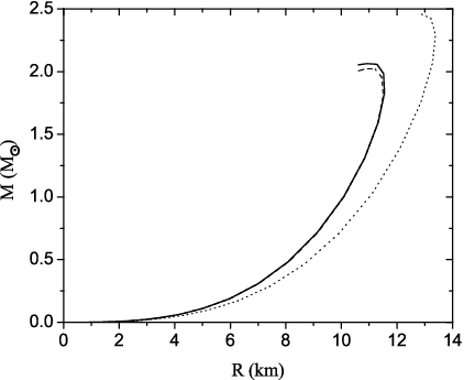
Even though the calculations in Fig. 7 should be considered as just an example, we see that the perpendicular pressure provides a “harder EOS” while the parallel is “softer”. Therefore, the former choice renders a higher maximum mass.
From those Figs. we conclude that one must restrict oneself to weak magnetic fields, when the deviation from spherical symmetry is very small (of order 0.001 %), in order to justify the use of Eqs. (33) and (34). If the magnetic field in these compact stars is too high, say G (at MeV), the spherically symmetric TOV equations cannot be employed because the deviations become important and lead to significant differences with respect of realistic axisymmetric models, yet to be constructed taking into account the pressure asymmetry. (this is why the M-R sequences in Fig. 7 lower panel should not be trusted, and we stress again that they should be considered just as an example). We shall address this issue elsewhere.
Fig. 8 compares our result for zero magnetic field EoS with the one presented in reference [8]. It shows that the curves calculated using NJL + B and bag model with small are quite similar. Nonetheless, it is important to stress that the calculations of the present work feature a self-consistent gap parameter (not a constant), which varies according to the particle density.
V.2 Hybrid Stars
The construction of models for the so-called “hybrid stars” faces the same problem as before when the magnetic-field-induced pressure anisotropy is considered. Working outside the stability windows render EoS which are valid only above a certain critical density, not all the way down to zero, since MCFL matter would be favored at high density only. Thus, the stellar models belong to the so-called hybrid type, in which a core of the high-density matter is present. Again, the value of the magnetic field induces an increasingly large anisotropy, which in turn forces the construction of axisymmetric (not spherical) stellar models. In this way, it can be modelled within the isotropic TOV formalism only for relative pressure differences in the ballpark of .
Fig. 9 displays a hybrid sequence obtained by employing the well-known Bethe-Johnson EoS for nuclear matter and using the Gibbs criteria for determining the value of the transition pressure between exotic and nuclear matter. These curves were calculated using the perpendicular pressure (for magnetized stars) as an example. As expected, the appearance of an MCFL core softens the EoS, rendering lower maximum masses than “pure” hadronic models. The main feature of considering the existence of magnetic field for hybrid MCFL stars is to switch the point where the hybrid sequences begin, i. e. where the stars start exhibiting a CFL core. Since the difference in the EoS for low field MCFL matter and CFL matter is of just a few percent (see Fig. 3), and because the star radius depends mainly on the nuclear EoS, observational data of maximum mass and minimum radii would not be able to distinguish the existence of low magnetic fields in these hybrid stars. Again, for high magnetic fields ( G) the results are still to be analyzed, but differences in the maximum allowed mass may arise, and therefore the results of spherical models cannot be trusted. This is potentially important for the identification of actual compact stars masses and radii [44] (see next Section).

VI Conclusions
We have shown that a magnetic field in CFL matter (termed MCFL phase here) does not, generally speaking, favor the stability scenario, and even forces a new condition (a field dependent vacuum “bag constant”) which is perhaps physically reasonable but cannot be verified as yet. However, absolute stability is not excluded provided the vacuum is properly modified by the magnetic field. On the other hand, in the absence of this dependence, we conclude that there is no room for absolute stability of CFL matter under the influence of a magnetic field within the model. If this is the case, there could be no magnetized “strange stars”, but only hybrid stars. Even before calculating stellar models in the anisotropic pressure regime, we can state that the found stability conditions can impose a maximum magnetic field that could be supported by self-bound MCFL strange stars (that is, stars made of this magnetized self-bound paired matter), a feature which in principle, could be compared with observations.
In the self-consistent approach used here for the gap parameter, we do not find much difference in the stability region at zero field as compared to the case in which the gap parameter is parameterized (and extended to quite high values) [8]. The EoS is still largely linear and substantially modified only at sufficiently high fields where the magnetized medium becomes highly anisotropic. It is not surprising then that in the quasi-isotropic regime ( G) the stellar sequences are not very different from the zero-field case (see Fig. 7).
We should notice that the anisotropic pressure regime is attainable at field values that are allowed in the core of compact stellar objects [18]. From the heuristic arguments presented in the Introduction, and then analytically and numerically corroborated in the paper, field effects become relevant in the EoS of MCFL matter for field strength . Nevertheless, for that field range the system asymmetry, expressed in terms of the pressure splitting , is significant, then invalidating the use of the TOV formalism. Thus, to work in the anisotropic regime, where the most interesting field effects should occur, an entirely different stellar structure formalism in agreement with the system cylindrical symmetry would be needed, since the spherical symmetry is broken from the very beginning by the presence of the strong magnetic field. We underline that the conventional TOV equations were obtained by solving the Einstein equations for a general time-invariant, spherically symmetric metric. That is, they were derived assuming spherically symmetric and isotropic medium in static gravitational equilibrium. Hence, it becomes imperative to generalize the TOV equations to an anisotropic medium employing a metric with cylindrical symmetry [49] that can accommodate the splitting of the longitudinal and transverse pressures appearing at strong enough magnetic fields. We expect to address this issue in a future publication.
It is important to stress that recent works [44]-[45] have exploited the increasing availability of high-quality data to pindown masses and radii of selected stellar systems. Even though the results and analysis are far from being definitive, there is evidence favoring a relatively soft EoS to model 4U 1608-52, 4U 1820-30 and EXO 1745-248 [45], at least in the region immediately above the saturation density. Comparing the prediction of our hybrid EoS model shown in Fig. 9 with the 1- and 2- confidence contours for the masses and radii of the three neutron stars in these binary systems, (shown in Fig. 1 of Ref. [45]), one can easily see that for fields within the isotropic regime our EoS is compatible with these observations.
On the other hand, recent measurements [46] of the Shapiro delay in the radio pulsar PSRJ1614-2230 have yielded a mass of . Even though such a large mass calls for a stiffer EoS, it does not rule out color superconductivity in the star’s core or a self-bound model like the curves in Fig. 7. In fact, by using the phenomenological EoS for quark matter proposed in Ref. [47], the authors of Ref. [48] showed that a large value of the star mass is only compatible with strongly interacting quarks paired in a color superconducting state. It is an interesting open question to explore, within the self-consistent approach used in our calculations, whether there is a physically viable region of the parameter space of the MCFL phase that can produce EoS curves compatible with the PSRJ1614-2230 mass observation.
Even if the measured systems do not possess a noticeable magnetic field, future determinations of SGR-AXN radii and masses are foreseeable. For those systems, an additional complication would arise with the consideration of the magnetic field, as discussed above. The particular case of MCFL elaborated here suggests that a full evaluation that takes into account the pressure anisotropy may be necessary to address masses and radii in the presence of very strong magnetic fields.
Acknowledgements.
L.P. and J.E.H. acknowledge the financial support received from the Fundação de Amparo à Pesquisa do Estado de São Paulo. They also thank UTEP for support and hospitality during three scientific visits in which this work was performed. J.E.H. also wishes to acknowledge the CNPq Agency (Brazil) for partial financial support. We thank Marcio G. B. de Avellar for useful discussions on mass-radius relation calculations. E.J.F. and V.I like to thank the Instituto de Astronomia, Geofísica e Ciências Atmosféricas, São Paulo, for the warm hospitality extended to them during their visit. The work of E.J.F. and V.I was supported in part by the Office of Nuclear Theory of the Department of Energy under contract DE-FG02-09ER41599.Appendix A Dynamical bag constant in the chiral limit at
Let us investigate the effect of an external magnetic field on the bag pressure found in Ref. [36]. In the dynamical approach of Ref. [36] the bag pressure has its origin in the spontaneous breaking of chiral symmetry. For our high density system the vacuum pressure contribution found in [36] reduces to taken in the chiral limit with
| (35) |
Here and are the current and dynamical quark masses respectively, and are quark self-interacting constants with dimensions and , respectively, and are the quark condensates given as functions of the corresponding quark dynamical masses by
| (36) |
with being the Fermi momenta depending on the densities .
A magnetic field modifies the expressions for the bag and the chiral condensates in the following way
| (37) |
and
| (38) |
where we assumed a magnetic field along the -direction, and used the notation: for the three-momentum, with labeling the discrete Landau levels, ; for the spin degeneracy of the Landau level; for the corresponding quarks’ electric charges; and for the integer part of the argument.
Comparing the leading term of (35),
| (39) |
with that of (37)
| (40) |
and taking into account that we have that the difference between and is basically due to the difference between the dynamical masses and condensates at zero and non-zero fields. That a magnetic field modifies the dynamical mass is a well known result in the literature [50]. However, as demonstrated in the NJL model for quark matter [51], and in the QCD chiral effective theory [52], the field-induced change in the dynamical masses and the chiral condensates are negligibly small for any field smaller than . This in turns translates into a negligible modification of the vacuum pressure by magnetic fields below . Hence, for the range of fields of interest for the astrophysics of compact stars, no significant field-induced variation of the vacuum pressure found in the framework of this approach will occur.
References
- [1] C. Alcock, E. Farhi and A. V. Olinto, Astrophys. J. 310, 261 (1986)
- [2] P. Haensel, J. Zdunik and R. Schaeffer, Astron. Astrophys. 160, 121 (1986); O. G. Benvenuto, J. E. Horvath and H. Vucetich, Int. Jour. Mod. Phys. A 6, 4769 (1991); M. A. Alpar, Phys. Rev. Lett. 58, 2152 (1987); N. K. Glendenning and F. Weber, Astrophys. J. 400, 647 (1992).
- [3] A. Bodmer, Phys. Rev. D 4, 1601 (1971); S. A. Chin and A. K. Kerman, Phys. Rev. Lett. 43, 1292 (1979); H. Terazawa, Tokyo U. Report., INS-336 (1979)
- [4] E. Witten, Phys. Rev. D 30, 272 (1984).
- [5] D. Bailin and A. Love, Phys. Rep. 107, 325 (1984), and references therein.
- [6] M. Alford, K. Rajagopal and F. Wilczek, Nuc. Phys. B537, 433 (1999); R. Rapp, T. Schaefer, E. V. Shuryak and M. Velkovsky, Ann. Phys. (NY) 280, 35 (2000); M. Alford, K. Rajagopal, S. Reddy and F. Wilczeck, Phys. Rev. D 64, 074017 (2001).
- [7] K. Rajagopal and F. Wilczeck, arXiv:hep-ph/0011333, and references therein.
- [8] G. Lugones and J. E. Horvath, Phys. Rev. D 66, 074017 (2002).
- [9] M. Alford, C. Kouvaris and K. Rajagopal, Phys. Rev. Lett. 92, 222001 (2004).
- [10] M. Alford, J. A. Bowers and K. Rajagopal, Phys. Rev. D 63, 074016 (2001); J. A. Bowers and K. Rajagopal, Phys. Rev. D 66, 065002 (2002); R. Casalbuoni and G. Nardulli, Rev. Mod. Phys. 76, 263 (2004).
- [11] P. F. Bedaque and T. Schafer, Nucl. Phys. A 697, 802 (2002); A. Kryjevski and T. Schafer, Phys. Lett. B 606, 52 (2005); A. Gerhold and T. Schafer, Phys. Rev. D 73, 125022 (2006).
- [12] M. Buballa, J. Hosek and M. Oertel, Phys. Rev. Lett. 90, 182002 (2003); A. Schmitt, nucl-th/0405076.
- [13] E. V. Gorbar, M Hashimoto, and V. A. Miransky, Phys. Lett. B 632, 305 (2006).
- [14] E. J. Ferrer and V. de la Incera, Phys. Rev. D 76, 114012 (2007).
- [15] I. Fushiki, E. H. Gudmundsson and C. J. Pethick, Astrophys. J. 342, 958 (1989); T. A. Mihara, et al., Nature (London) 346, 250 (1990); G. Chanmugam, Ann. Rev. Astron. Astrophys 30, 143 (1992); J. H. Taylor, R. N. Manchester and A. G. Lyne, Astrophys. J. Supp. 88, 529 (1993); P. P. Kronberg, Rep. Prog. Phys. 57, 325 (1994); D. Lai, Rev. Mod. Phys. 73, 629 (2001); D. Grasso and H. R. Rubinstein, Phys. Rep. 348, 163 (2001).
- [16] C. Thompson and R. C. Duncan, Astrophys. J. 392, L9 (1992), ibid 473, 322 (1996); S. Kulkarni and D. Frail, Nature 365, 33 (1993); T. Murakami et al., Nature 368, 127 (1994); Ibrahim et al., Astrophys. J. 609, L21 (2004).
- [17] E. J. Ferrer and V. de la Incera, Phys. Rev. Lett. 97, 122301 (2006); T. Tatsumi, T. Maruyama, E. Nakano and K Nawa, Nucl. Phys. A774, 827 (2006); D.T. Son and M.A. Stephanov, Phys. Rev. D 77, 014021 (2008).
- [18] E. J. Ferrer, et al., Phys. Rev. C 82, 065802 (2010).
- [19] M. Alford, J. Berges and K. Rajagopal, Nucl. Phys. B571, 269 (2000); E. V. Gorbar, Phys. Rev. D 62, 014007 (2000); R. Casalbuoni and R. Gatto, Phys. Lett. B 464, 111 (1999).
- [20] E. J. Ferrer, V. de la Incera, and C. Manuel, Phys. Rev. Lett. 95, 152002 (2005).
- [21] E. J. Ferrer, V. de la Incera, and C. Manuel, Nucl. Phys. B 747, 88 (2006).
- [22] E. J. Ferrer, V. de la Incera, and C. Manuel, J. Phys. A39, 6349 (2006).
- [23] Sh. Fayazbakhsh, N. Sadooghi, Phys. Rev. D82, 045010 (2010).
- [24] E. J. Ferrer and V. de la Incera Phys. Rev. D 76 045011 (2007).
- [25] M. Alford and S. Reddy, Phys. Rev. D 67, 074024 (2003).
- [26] M. Baldo, et al., Phys. Lett. B 562, 153 (2003); D. Blaschke, S. Fredriksson, H. Grigorian, and A. M. Oztas, Nucl. Phys. A 736, 203 (2004); S. B. Ruester, and D. H. Rischke, Phys. Rev. D 69, 045011 (2004); A. Drago, A. Lavagno, and G. Pagliara, Phys. Rev. D 69, 057505 (2004); M. Alford, M. Brady, M. W. Paris, and S. Reddy, Astrophys. J. 629, 969 (2005); G. Lugones, and I. Bombaci, Phys. Rev. D 72, 065021 (2005); D. Page, and S. Reddy, Ann. Rev. Nucl. Part. Sci. 56, 327 (2006); B. K. Sharma, P. K. Panda, and S. K. Patra, Phys. Rev. C 75, 035808 (2007); M. Alford, et al., Nature (London) 445, E7 (1007); G. Pagliara, and J. Schaffner-Bielich, Phys. Rev. D 77, 063004 (2008); B. K. Agrawal, and S. K. Dhiman, Phys. Rev. D 79, 103006 (2009).
- [27] M. Alford, Physics 3, 44 (2010).
- [28] A. Broderick, M. Prakash, and J. M. Lattimer, Astrophys. J. 537, 351 (2000).
- [29] E. J. Ferrer, and V. de la Incera, Phys. Rev. D 76, 045011 (2007).
- [30] J. L. Noronha and I. A. Shovkovy, Phys. Rev. D 76, 105030 (2007).
- [31] K. Fukushima and H. J. Warringa, Phys. Rev. Lett. 100, 032007 (2008).
- [32] M. Alford, C. Kouvaris and K. Rajagopal, Phys. Rev. D 71 054009 (2005).
- [33] V. Canuto, and J. Ventura, Fund. Cosmic Phys. 2 (1977) 203; I. Fushiki, E. H. Gudmundsson, and C. J. Pethick, Astrophys. J. 342 (1989) 958; A. M. Abrahams and S. L. Shapiro, Astrophys. J. 374 (1991) 652; I. Fushiki, et al., Ann. of Phys. (NY) 216 (1992) 29; Rögnvaldsson et al., Astrophys. J. 416 (1993) 276; S. Chakrabarty, D. Bandyopadhyay, and S. Pal, Phys. Rev. Lett. 78 (1997) 2898; D. Bandyopadhyay, et al. Phys. Rev. D 58 (1998) 121301; C. Y. Cardall, M. Prakash, and J.M/ Lattimer, Astrophys. J. 554 (2001) 332; I.-S. Suh, and G.J. Mathews, Astrophys. J. 546 (2001) 1126; V.R. Khalilov, Phys. Rev. D 65 (2002) 056001; F.X. Wei, et al. J. Phys. G 32 (2006) 47; A.K. Hardings and D. Lai, Rep. Prog. Phys. 69 (2006) 2631; W. Chen, P.-Q. Zhang, and L.-G. Liu, Mod. Phys. Lett. A 22 (2007) 623; A. Rabhi, C. Providencia, and J. Da Providencia, J. Phys. G 35 (2008) 125201; F. Yang, H. Shen, Phys. Rev. C 79 (2009) 025803, A. Perez-Martinez, H. Perez-Rojas, and H. J. Mosquera-Cuesta, Eur. Phys. J. C29 (2003) 111;
- [34] S. Chakrabarty, Phys. Rev. D 54, 1306 (1996); M. Chaichian, et al. Phys. Rev. Lett. 84 (2000) 5261; R. Gonzalez-Felipe, A. Perez-Martinez, H. Perez-Rojas, and M. Orsaria, Phys.Rev.C 77 (2008) 015807; D.P. Menezes, et al., Phys. Rev. C 79 (2009) 035807; D. P. Menezes, et al., Phys. Rev. C 80 (2009) 065805; A. Rabhi, et al., J. Phys. G 36 (2009) 115204.
- [35] V. I. Ritus, Ann.Phys. 69, 555 (1972); Sov. Phys. JETP 48, 788 (1978) [Zh. Eksp. Teor. Fiz.75, 1560 (1978)]; E. Elizalde, E. J. Ferrer, and V. de la Incera, Ann. of Phys., 295, 33 (2002).
- [36] M. Buballa, Nucl. Phys. A 611, 393 (1996); M. Buballa and M. Oerted, Phys. lett. B 457, 261 (1999).
- [37] P. Rehberg, S.P. Klevansky, J. Hüfner, Phys. Rev. C 53, 410 (1996).
- [38] M. G. Alford, Ann.Rev.Nucl. Part. Sci. 51, 131 (2001) [arXiv:hep-ph/0102047]; G. Nardulli, Riv. Nuovo Cim. 25N3, 1 (2002) [arXiv:hep-ph/0202037].
- [39] L. D. Landau and E. M. Lifshitz, The Classical Theory of Fields Elsevier Butterworth-Heinemann (Four Edition, 1975) MA, Ch. 11 (pp. 290-293).
- [40] D. Ebert, K.G. Klimenko, M.A. Vdovichenko, A.S. Vshivtsev, Phys. Rev. D61, 025005 (2000); D. Ebert, K.G. Klimenko, Nucl. Phys. A728, 203 (2003).
- [41] R. Gonzalez Felipe, D. Manreza Paret and A. Perez Martinez, Magnetized color flavor locked state and compact stars, arXiv:1003.3254 [astro-ph.HE].
- [42] E. Farhi and R. L. Jaffe, Phys. Rev. D 30, 2379 (1984).
- [43] B. Müller and J. Rafelski, Phys. Lett. B 101, 111 (1981); S. Pal, et al., Phys. Rev. C 60, 015802 (1999); R. Aguirre, Phys. Lett. B559, 559 (2003); N. Prasad and R.S. Bhalerao, Phys. Rev. D69, 103001 (2004); O. E. Nicotra, M. Baldo, G. F. Burgio, H.-J.Schulze, Phys. Rev. D 74, 123001 (2006).
- [44] F. Ozel and D. Psaltis, Phys. Rev. D 80, 103003 (2009).
- [45] F. Ozel, G. Baym and T. Guver, Phys.Rev.D 82, 101301 (2010).
- [46] P. Demorest, T. Pennucci, S. Ransom, M. Roberts, and J. Hessels, Nature, 467, 1081 (2010).
- [47] M. Alford, M. Braby, M. Paris, S. Reddy, ApJ. 629, 969 (2005).
- [48] F. Ozel, D. Psaltis, S. Ransom, P. Demorest, and M. Alford, Ap. J. Lett. 724, 199 (2010).
- [49] T. Lewis, Proc. Roy. Soc. (London) A136, 176 (1932); L. Marder, Proc. Roy. Soc. (London) A244, 524 (1958); M. A. Melvin, Phys. Lett. 8, 65 (1964); K. S. Thorne, Phys. Rev. 138, B25 (1965); J. I. Safko and L. Witten, J. Math. Phys. 12, 257 (1971); M. M. Som, A.F. da Teixeiraand and I. Wolk, Acta Physica Austriaca 43, 15 (1975); P. S. Letelier and R. R. Tabensky, IL Nuov. Cimento, 28B, 408 (1975); M. M. Som and N.O. Santos, Braz. Jour. Phys., 8, 368 (1978); P. S. Letelier, Joun. Math. Phys. 16, 1488 (1975), ibed 20, 2078 (1979); S. Prakash and S. R. Roy, J. Phys A13, 3773 (1980); S.R. Roy and S. Narain, Int. Journ. of Theor. Phys. 20, 709 (1981); R. Bali and A. Tyahi, Astrophys. and Space Sci. 185, 299 (1991).
- [50] K. G. Klimenko, Z. Phys. C 54, 323 (1992); K. G. Klimenko, Teor. Mat. Fiz. 90, 3 (1992); V. P. Gusynin, V. A. Miransky and I. A. Shovkovy, Phys. Rev. Lett. 73, 3499 (1994); Nucl. Phys. B563, 361 (1999); C. N. Leung, Y. J. Ng and A. W. Ackley, Phys. Rev. D 54, 4181 (1996); D. S. Lee, C. N. Leung and Y. J. Ng. Phys. Rev. D 55, 6504 (1997); E. J. Ferrer and V. de la Incera, Phys. Rev. D 58, 065008 (1998); Phys. Lett. B 481, 287 (2000); Phys. Rev. Lett. 102, 050402 (2009); Nucl. Phys. B824, 217 (2010).
- [51] K. G. Klimenko and V. Ch. Zhukovsky, Phys. Lett. B 665, 352 (2008).
- [52] I. A. Shushpanov and A. V. Smilga, Phys. Lett. B 402, 351 (1997); N. O. Agasian and I. A. Shushpanov, Phys. Lett. B 472, 143 (2000); T. D. Cohen, D. A. McGady and E. S. Webos, Phys. Rev. C 76, 055201 (2007); E. S. Werbos, Phys. Rev. C 77, 065202 (2008).