Stochastic modeling of gene activation and application to cell regulation
Abstract
Transcription factors (TFs) are key regulators of gene expression. Based on the classical scenario in which the TF search process switches between one-dimensional motion along the DNA molecule and free Brownian motion in the nucleus, we study the arrival time of several TFs to multiple binding sites and derive, in the presence of competitive binding ligands, the probability that several target sites are bound. We then apply our results to the hunchback regulation by bicoid in the fly embryo and we propose a general mechanism that allows cells to read a morphogenetic gradient and specialize according to their position in the embryo.
Keywords: modeling, stochastic binding, diffusion of transcription factor, gene activation, morphogenetic gradient, cell differentiation.
1 Introduction
Transcription factors (TFs) are key regulators that can initiate or inhibit gene activation by binding to specific DNA sites. TFs enter the cell nucleus and search for their specific binding sites on the DNA molecule. In a context of competition for activation and inhibition, the search for target sites should not be too long otherwise, another gene might be activated. This is the case for olfactory gene activation [1], where a single G-coupled receptor out of hundreds is expressed in a single cell, while all other receptors are repressed. Thus cells might use various mechanisms to control gene activation including changing local properties of the DNA molecule (for example by methylation or acetylation) or changing the properties of the TF interaction as what happens when specific molecules bind to TFs and modify their affinity for the DNA molecule.
The mean time to reach a target site is thus a fundamental parameter of gene activation and several biophysical scenarios have been proposed to estimate it. Berg and Von Hippel [2, 3, 4] realized that the search time cannot be computed using a three dimensional random walk only, because the observed search time is indeed shorter. Using the property that the TF scans the DNA base pairs for potential binding sites, they proposed that the search consists of consecutive cycles of three dimensional free diffusion in the nucleus and one dimensional random motion along the DNA molecule. DNA base pairs are not electrically charged and so no long distance interactions are involved, thus, the TF should physically come close to the DNA in order to generate a true interaction. During the one dimensional search, the TF is confined to a neighborhood of the DNA molecule and can detach due to thermal fluctuations and a new 1d-3d cycle resumes until the target is eventually reached. This basic scenario has been confirmed experimentally by single particle tracking experiments [21] and investigated theoretically, by accounting for the local base pair interactions, the mean number to scan the base pairs per cycle, the free diffusion time and the time the TF is bound to the DNA molecule [5, 6, 7, 8, 10].
However, it is still unclear how to go from the TF search time to the mechanism responsible for cell specialization. Cells in a living tissue are imbedded in a matrix of positional information, generated by morphogenetic gradients [11, 12, 13, 14, 15]. A first step consists of the ability of the cell to ”read out” the local characteristics of the morphogenetic gradient so that the cell can be labeled and acquire its own identity. To address this question, here we investigate how several binding sites can be bound at steady state by several TFs generated by an external steady state gradient. In particular, we are led to compute the mean time for some TFs to bind to many target sites. The number of bound sites can be seen as a digital-converter used by the cell to discriminate two different morphogenetic gradient concentrations depending whether or not all the binding sites are saturated. We further study the effect of competitive ligands that can modulate the TF’s action leading to gene repression.
First, we present our computation for the time for a single TF to bind to one of multiple potential binding sites. The distribution of the arrival time is always a sum of two exponentials but, for a large number of free diffusion and DNA binding cycles, the arrival time is single exponentially distributed. We then expand our analysis to multiple TFs with multiple targets in the presence of enzymes leading to degradation. We apply our results to estimate the number of active sites when the cell nucleus experiences a steady state TF influx. Finally, we estimate the steady state probability that a given number of binding sites are occupied. In our model, this probability describes the proportion of time a gene is actively transcribed. We apply our analysis to the initial patterning of the fly embryo by the bicoid (bcd) morphogenetic gradient. The bcd gradient regulates a number of downstream TFs involved in the gap gene network [16, 17], which determines the position of body sections along the anterior-posterior (A-P) axis in the drosophila embryo. Among these gap genes, hunchback (hb) is responsible for thoracic development [16, 17]. Hb activation leads to the formation of a sharp boundary and to the formation of stripes. We use our analysis of TF binding to determine the hb density induced by bcd activation, and we show that this hb-bcd interaction-modulation is sufficient to generate the transition from a smooth bicoid gradient into a sharp hb boundary in the middle of the drosophila embryo. Our approach provides a general scenario at a molecular level of TF interactions that lead to cell specialization.
2 Distribution and mean of the search time
We first summarize the properties associated with the TF’s search process to its binding site. The TF switches between a free diffusion and random walk along the DNA molecule [2, 5, 9, 10].
- 1.
Due to the interaction potential with the DNA backbone [18], the TF can bind unspecifically to the DNA molecule. The strength of the interaction potential is around [19, 5], larger than the thermal noise . In this deep well approximation, the random time a TF stays bound is exponentially distributed [20]. Experimental and theoretical estimates for the average time are in the range of a few milliseconds [21, 10].
- 2.
- 3.
A TF can detach from the DNA due to thermal noise and diffuse freely in the nucleus until it rebinds to the DNA. When the DNA molecule occupies a small fraction of the nucleus and can be approximated as long rods, the random time a TF spends diffusing in the nucleus is exponentially distributed [10] with an average , which is on the order of a few milliseconds [21, 10]. However, for larger density and a complex DNA organization, the distribution time in general is a sum of exponentials and might even be more complicated.
We start with copies of a TF, alternating independently between periods of free diffusion and random walks along the DNA until one of the binding sites is found. We further consider competitive ligands that can bind to the TF target sites, preventing the sites to be occupied by TFs. The ligand binds to the target site according to a first order reaction:
| (1) |
with an association and a dissociation rate and respectively. At equilibrium, Michaelis-Menten reaction says that for a concentration of ligands, the probability that a binding site is not occupied is:
| (2) |
Search time for a single TF
The random time for a single TF to bind to a target site is the sum of the time spent in one and three dimensions. Using the characteristic function of the search time , we can express the probability density function (pdf)
| (3) |
as follows (see appendix):
| (4) |
where and are the two positive roots of and is the probability to find a target during a single one dimensional walk along the DNA. The associated mean binding time is:
| (5) |
In the limit , using the expression for the two roots and approximating the pdf (eq. 4) by a single exponential for a time t such that (see appendix), we obtain that
| (6) |
Since and are both on the order of a few ms [10, 21], the single exponential limit is valid for larger than a few ms. The mean time then reduces to
| (7) |
The mean number of free diffusions and DNA bindings before finding the target site is equal to . The limit corresponds to TFs that find their target sites after a large number of cycles.
Search time for multiple TFs
When there are TFs that can potentially bind to identical binding sites (a site can only be occupied by a single TF), in the single exponential limit, the time for the first TF to bind a site is the minimum of the exponential laws of mean time . is then exponentially distributed with mean:
| (8) |
We shall consider well separated sites (by at least a distance of base pairs). In this case, the probability to find each site during a DNA biding is where is the total number of base pairs in the genome. Furthermore, in the presence of competitive ligands, there are available binding sites. Thus, the probability of binding to one of the sites is and the mean binding time for well separated sites with is:
| (9) | |||||
| (10) |
where
| (11) |
is the search time for a single TF with a single target site.
Remark 1. Formula (10) describes the combined effect of multiple but well separated binding sites. When the sites are clustered, the mean time to find a target becomes a nonlinear function of the distribution [23, 24, 25, 26, 27] and has been approximated by the Berg-Purcell approximation formula [28]. When there are binding sites of size , located on an ensemble of DNA-molecules on a sphere of radius R, the mean time in 3d to find a site is:
| (12) |
This formula can be improved [29, 30]. Here is an effective diffusion constant that accounts for the switch between the 1D DNA motion and the 3D diffusion. When the one 1D excursion length is small compared to the 3D diffusion length,
| (13) |
In the other cases, one has to deal with random jumps.
3 From a morphogenetic gradient to DNA site activation
We shall now apply our previous results to estimate the number of occupied sites when a nucleus receives a steady influx of TFs. This steady influx of TFs entering the nucleus could, for example, either be imported from outside the cell or be steadily produced in the cytoplasm of the cell. We consider that gene expression is proportional to the mean time the binding sites are occupied. Since the number of binding sites occupied controls gene expression, we shall estimate, for a given TF influx, the mean proportion of time the binding sites are occupied.
3.1 Activation of a single binding site
We first compute the average occupation ratio of a single binding site before considering multiple sites in the following section. To compute , we use Bayes’ law and sum over the number of TFs in the nucleus:
| (15) |
where is the probability of having TFs in the nucleus and is the conditional probability that a single binding site is occupied when there are TFs. To proceed with the computation of , we assume that TFs arrive in the nucleus at a Poissonnian rate and are degraded (free or bound) by enzymes at a rate . Thus, the number of TFs in the nucleus follows a birth and death process and is distributed according to a Poisson law with mean :
| (16) |
We now compute . When a TF has found the target, it stays attached for a mean time . We consider that the rate of binding and unbinding to the sites is faster than the rate of TF turn over in the nucleus and that the steady state between binding and unbinding is reached, thus
| (17) |
where Using equations (15), 16 and (17), we get:
| (18) |
Using we obtain:
| (19) | |||||
where . We plot in figure 1a the occupation ratio as a function of the average number of TFs in the nucleus for different values of . When the competitor ligand concentration varies, the occupation ratio is modulated as described in figure 1b. Using Lac I data [21] and in the absence of DNA binding competitor (), the total search time is [21, 10], while [32] and thus the ratio is . We conclude (red curve Fig 1a) that for low , the target site can be occupied for a significant proportion of time. In particular, small fluxes of TFs can induce significant modifications on gene expression in a target cell.


3.2 Activation with multiple binding sites
When there are binding sites, we shall now compute the proportion of time that sites are occupied. Using Bayes’ law, we have:
| (20) |
where is the probability to have TFs given by expression (16). We now compute by analyzing a Markov chain [33] which describes the probability that q sites are occupied at time .
When sites are occupied, the total release rate is while the arrival rate to a site is given by with equation (11). The forward and backward rate of the Markov chain are given by:
| (21) | |||||
| (22) |
and the Markov chain is given by [33]:
| (23) |
with the boundary conditions:
| (24) | |||||
| (25) |
We consider that the rate of binding and unbinding to the sites is faster than the rate of TF turn over in the nucleus and that the steady state is achieved quickly, thus:
| (26) |
where By induction [33], for (the maximal number of sites occupied by TFs), we get:
| (27) |
where:
| (28) |
For , since there can be no more than TFs bound. Using the normalization condition,
| (29) |
we finally get for :
| (30) |
and for :
| (31) |
Using expressions (16), (20) and (27), we obtain for :
| (32) |
and for :
| (33) |
and for as there can not be more than TFs bound to the target sites. We shall now derive asymptotic expressions for when and , which correspond respectively to a small average number of TFs in the nucleus and to TFs that stay bound to the targets a long time compared to the search time.
Asymptotics for small
With the expression of given in (16) and the summation (20), only the terms contribute to the first order asymptotic in . With (27) we obtain:
| (34) |
and with ,
With (20), for ,
| (35) |
We conclude that the probability that one site is occupied is given by the average number of TFs multiplied by the probability to have one site occupied when there is one TF in the nucleus.
Asymptotic for small
We now compute the asymptotic for .
- 1.
When the number of TFs is larger than the number of available sites (), using equation (30), for , only the terms and contribute to the first order for . Using the normalization relation (29),
Furthermore with (30),
we then obtain:
(36) (37) We ignore all other probabilities in the first order for . When and almost all sites are occupied.
- 2.
When there are less TFs than the number of available sites (), then for only and have a contribution in the leading order of equation (30). We obtain:
(38) (39) We neglect all other probabilities in the first order for .
Combining equations (16), (20) and the first order approximations in , the probability that all sites are simultaneously occupied is:
| (40) |
Using the partial sum:
| (41) |
and after some computation (see appendix) we can write:
| (42) |
For , is an increasing function of and a decreasing function of (see appendix). Increasing the number of TFs leads to an increase in the probability that all sites are occupied, while increasing decreases the probability that all sites are occupied.
Similarly (see appendix), with equations (95), (94) and (42) the asymptotic expression of the occupation ratio for is given by:
We plot in figure 2 (resp. 3) the function as a function of for (resp. ).


3.3 Consequence of the analysis for gene expression stability
We now use our results on the occupation ratios to show that at least two binding sites are required for the regulation of a genetic switch. A genetic switch is a special type of autoregulated gene. These autoregulated genes code for TFs that regulate the transcription of their own gene. A genetic switch is a process allowing two stable values for the transcription rate of a gene [34]: an ”on” position where the gene is transcribed and an ”off” position where it is not transcribed. If the gene is ”on”, transcription is maintained at high levels through autoregulation. If the gene is ”off”, transcription remains at low levels and does not turn on without an external signal. Genetic switches play a central role in cellular differentiation, memory and plasticity [35, 36].
We shall show that a bistable genetic switch can only appear when there are at least two binding sites regulating the transcription of the gene. We first determine the steady state concentration of the TF due the balance of production and degradation by enzymes. For a gene transcribed at a rate when there are occupied binding sites, the steady state production of TFs verifies:
| (47) |
where is given by formula (3) and depends on and . The steady state value satisfies the nonlinear equation:
| (48) |
where . Bistability appears when equation (48) has two stable solutions, thus equation (48) must have three solutions (two stable and one unstable in between). The number of solutions depends on the parameters and : For , as plotted in figures 2 and 3, has only one solution. For , has one solution for small and two solutions for large. For , using formula (3) and as plotted in figures 2 and 3, is a sigmoid type function. For sufficiently large, equation (48) has three solutions (figure 2) and two of them are stable. A gene following such activation properties is a bistable switch. Conversely, for sufficiently small, is the only stable solution. The critical value of can be characterized geometrically, as the point where is tangent to . For this critical value there is a stable point at the origin and a saddle point at the tangent point. To conclude, a bistable switch requires at least two binding sites regulating the gene and the parameter must be sufficiently large.
4 Formation of the Hunchback boundary by the Bicoid gradient
We shall now apply our analysis to determine the formation of the Hunchback TF (hb) boundary by the Bicoid (bcd) morphogen gradient in the drosophila embryo. The bcd gradient regulates a number of downstream TFs involved in the gap gene network [16, 17], which determine the position of body sections along the anterior-posterior (A-P) axis in the drosophila embryo. Among these gap genes, hb is responsible for thoracic development [16, 17]. Given a bcd gradient, we propose to determine the spatial distribution of hb. Our analysis shows how a broad bcd gradient can trigger a sharp transition in the hb density in the middle of the embryo. We reproduce the bcd and hb density measured in vivo [16] in figure 6a. To distinguish the values of and for the hb and bcd TFs required in our previous model, we shall use subscript h for the hb TF and b for the bcd TF. We approximate bcd gradient as exponential [16]:
| (49) |
where is the normalized A-P position ( where L is the length of the drosophila embryo). We use , corresponding to the best fit for the in vivo data [16]. The constant cannot be obtained directly from in vivo data. However, since
| (50) |
changing the value of is equivalent to an x-translation of the hb and bcd densities. We choose such as the hb boundary is in the middle of the drosophila embryo (see figure 4b).
hb transcription results from the binding of the hb TF and the bcd TFs to a promoter with 6 bcd binding sites and 2 hb sites [37, 38, 39]. Hb is transcribed at a rate when there are two hb or at least one bcd bound to the sites, described as
The hb density is proportional to the steady state production of hb given by , where
| (51) |
is the probability that hb is not transcribed, is the probability that no bcd are bound to the promoter and the probability that there are not two hb bound. At equilibrium, using , we obtain the steady state equation
| (52) |
where and is the degradation constant for hb. Equation (52) is implicit for the mean number of hb, that we shall now compute. We will now evaluate separately expressions and Along the A-P axis parameterized by the position , depends on the mean number of bcd TFs and on the ratio of the search time of bcd over the binding time. To evaluate , we use the binding reaction of a bcd to its target site :
| (53) |
where is the bcd TF bound to its target site. The equilibrium constant is the ratio of the forward to the backward rate of (53), equivalently:
| (54) |
For [40], a nucleus of volume and with the Avogadro number we obtain
To compute , we use formula (3) with and obtain:
| (55) |
We shall now evaluate the probability . In the absence of any precise data on the dissociation constant of hb from its binding site, we consider that binding is fast enough so that . Using expression (3) for the probability with , we obtain
| (56) |
Finally, at steady state, the equilibrium condition (52) reads:
| (57) |
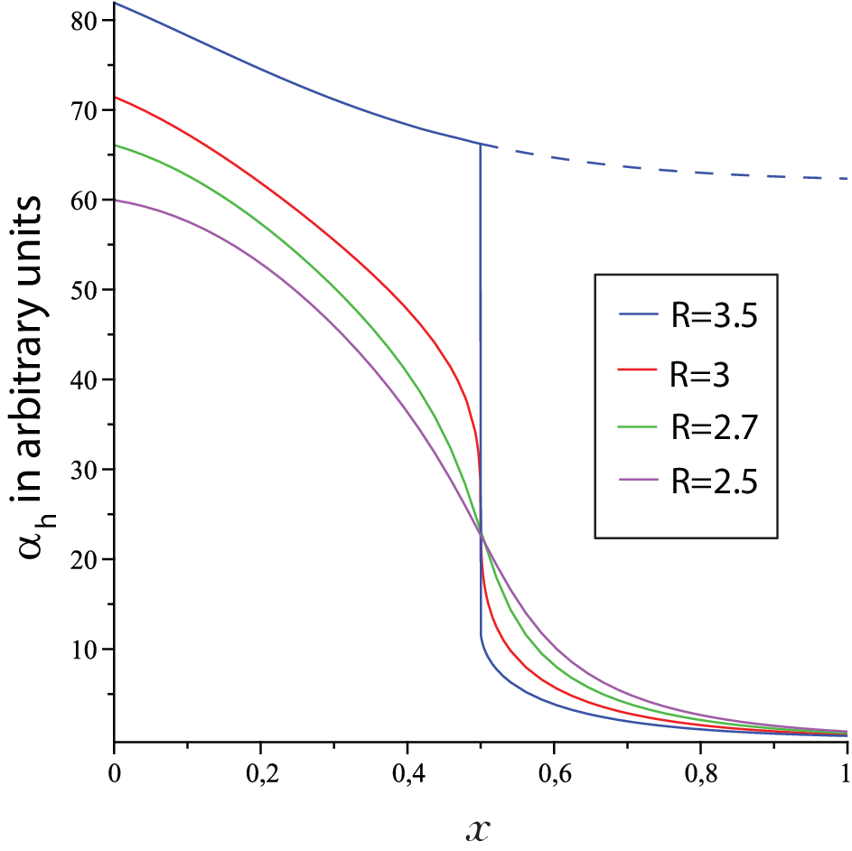
We solve equation (57) numerically (with Maple) to express as a function of . We plot in figure 4a-b several solutions associated with different values of and . As pointed out in equation (49) and plotted in figure 4a, changing the value of is equivalent to a x-translation of the hb and bcd densities. To further study the different types of solutions, we will vary the parameter . Following the discussion in section 3.3 on bistability, for the dynamics for hb can potentially be bistable. We show now that for and , hb is always monostable. To compute the critical value after which bistability occurs, we shall use the functions:
| (58) | |||||
| (59) |
where depends on through (49). The function is the fraction of time hb is autoactivated by the hb and is the fraction of time the gene is activated by the bcd gradient. Equation (57) can then be rewritten as:
| (60) |
We determine in the appendix the critical value for bistability given by . For the gene is always monostable, while for the gene is bistable for some values of and monostable for others:
- •
For , hb is monostable for and bistable for where is a critical position. We represent the bifurcation diagram in figure 4d. Changing is equivalent to an x-translation in the hb profile and thus can be adjusted such as the bifurcation point is for example. If at time there is no hb, the hb density converges to the lower stable value, as represented in figure 4b. Nevertheless, for a bistable hb dynamic, cells located in can switch from the low to the high stable value for a sufficient perturbation. In the absence of a repressor of hb on the posterior side of the embryo, these cells would stay in the high stable state.
- •
For , hb is always monostable. When becomes close to 3, there is already a boundary in the hb density (figure 4b). This boundary can be characterized by the point where changes concavity and becomes tangent to a linear function (figure 5). At the point of concavity change, a small variation in induces a large variation in which produces a sharp transition in the hb density.
We conclude that for an auto-regulated hb gene, when the bifurcation parameter is close but smaller than the critical value , there is a sharp boundary of hb in the embryo and this boundary does not require a repressor in the posterior half of the embryo. As shown in figure 5, at the boundary hb synthesis is essentially due to autoactivation of hb (the activation due to bcd is whereas the gene is autoactivated of the time). To obtain a numerical estimation of , we use the synthesis rate generated by two hb bound to the target sites and the degradation rate of hb. Using the values from the supplementary material of [37], and and we obtain
| (61) |
For , we observe a steep transition of the hb density at the middle of the embryo as in the in vivo data from [16] reproduced in figure 6a. The main difference between the theoretical density (figure 4b) and the in vivo data from [16] (figure 6a) is in the anterior edge where our model leads to an increase of the hb density instead of a decay as observed in vivo. This decay in the hb density at the anterior edge of the embryo is due to a repressive effect induced by the huckebein TF (hkb) [17] which we did not model in (57) and we shall examine now.



Refining the gradient using hkb repressor
We now account for the repression induced by hkb and consider that the transcription of the hb gene is repressed when at least one hkb is bound to the promoter site. Similarly to the analysis that lead us to equation (52), we obtain:
| (62) |
where is the probability that no hkb are bound. We assume hkb binds to its target fast enough and shall consider that . Finally, is then given by:
| (63) |
To evaluate the distribution we fit the measured hkb distribution [17] with an exponential function:
| (64) |
where (see figure 6c). The value of can not be obtained directly from experimental measurements. Changing the value of is equivalent to an x-translation of the repression due to hkb. We calibrated to have the same value for the hb density as in the vivo data (fig 6a and d). We solve equation (62) numerically and obtain an hb density represented in figure 6b. This new theoretical density obtained is now close to the in vivo data (figure 6a), in particular we recover the sharp boundary of hb. The main differences between the theoretical and experimental densities are located at the posterior side of the hb boundary where we obtain a higher density than the vivo data and at the posterior edge where the density is lower. The difference at the posterior side of the hb boundary might be due to repression of hb by the knirps TF [17] which is not modelled here. As for the difference at the posterior edge, this can be due to activation of hb by the Caudal TF [17]. Taking into account these two regulation pathways should lead to a refined analysis of the hb density.


5 Conclusion
In this paper, we studied transcription activation by TFs starting from the stochastic nature of the search process for a DNA promoter site. We then applied our computations to estimate the sharp boundary induced by a smooth gradient of TFs. In the first part, we focused on the kinetics of the binding of TFs to their target sites located on the DNA molecule: when the average number of cycles of free diffusions and DNA bindings before finding the target sites is large, the search time is exponentially distributed and we estimate the mean (relation (10)). Next, we considered the case of a cell receiving a steady state influx of TFs which can be enzymatically degraded. We modeled the dynamics of the TFs’ binding and unbinding their target sites and we estimated the fraction of time that out of sites are occupied at steady state. For we obtain an explicit expression in equation (19). For , the general expression of is given by an equation (32) and an asymptotic development for is provided in expression (3). We presented the different occupation ratios in figure 2 and 3 for two and four sites respectively. We consider that the transcription rate is proportional to the fraction of time a given number of sites are occupied. For a defined TF concentration entering the nucleus, our model provides a quantitative input-output relation in terms of the transcription rate.
When we apply our model to the regulation of hunchback by the bicoid morphogenic gradient, we focus on the sharp boundary in the hb density at the middle of the embryo. Several mechanisms accounting for the formation of sharp boundaries have been proposed: Some mechanisms [40, 43, 44, 45] result from cooperative binding while others include a bistable gene [37] or the antagonistic action of a repressor and activator gradient [46, 47, 48, 49]. Here, we use neither the repression of hb in the posterior half nor the cooperative binding of bcd, but we show that, in the absence of these two mechanisms, a smooth morphogenetic gradient can trigger a sharp boundary for an autoregulated gene. We also show that bistability of the autoregulated gene is not a requirement and that sharp boundaries can be generated by monostable autoregulated genes. We found the critical value for the transcription rate at which a bifurcation occurs and gave an estimate in equation (105). We further show that a bistable gene can produce a sharp boundary from a smooth gradient. Nevertheless, for a bistable hb, cells located on the posterior side of the embryo can switch from a low stable value to a high one in response to a sufficiently large perturbation. A repressor on the right hand side of the boundary would then be required to obtain a reliable boundary position. Our results show that an autoregulated gene close to bistability is sufficient to produce a sharp boundary.
Here, we focused on a minimal mechanism that allows a morphogenetic gradient to trigger a sharp boundary in an autoregulated gene. In order to focus on this minimal system that produces sharp boundaries, neither hb-repression in the posterior half nor cooperative binding of bcd are modeled. Both repression [46] and cooperative binding [43] are already known to play a key role in the formation of the sharp boundary of hunchback and it would thus be interesting to expand our model to take them into account. With autoregulation, it would then be interesting to see how these three mechanisms, which appear to be redundant, produce sharp and robust boundaries in the embryo.
6 Appendix
6.1 The pdf of
We compute here the pdf of the time a single TF takes to bind one of the DNA specific targets. Decomposing the pdf by the event that the target is found after exactly k steps, we have:
| (65) |
Using the probability to bind to one of the sites during a one dimensional motion along the DNA molecule, the probability to find a site during the one dimensional DNA motion is given by:
| (66) |
A cycle is the concatenation of one and three dimensional motions. Both periods are characterized by random exponential times. The conditional search time for cycles of DNA binding and free diffusion is then:
| (67) |
where and are respective the times spent bound to the DNA and freely diffusing in the nucleus.
To compute , we will use the characteristic function of ,
| (68) | |||||
| (69) |
where is the characteristic function of . Since the random times and are independent, the characteristic function of the sum (67) is the product of the characteristic functions:
| (70) |
where and are respectively the characteristic functions of the free diffusion time and the time bound to the DNA. Since these times are exponentially distributed:
| (71) | |||
| (72) |
Finally,
| (73) | |||||
| (74) |
The poles are given by the two roots of with :
| (75) | |||
where, for , the two roots and are real positive. Decomposing the fraction (74) gives:
| (76) | |||||
| (77) |
where comes from the equation satisfied by and . By inverting the characteristic function and since the inverse transform of is an exponential distribution of mean , we obtain:
| (78) |
We conclude that the distribution is the sum of two decreasing exponentials.
6.2 Asymptotic pdf of for
We shall now study the approximation , for which:
| (79) | |||||
| (80) |
and
| (81) |
with . Since the second exponential converges faster to than the first and is further multiplied by a small coefficient .
6.3 Computation of for
Combining equations (16), (20) and the first order approximations in , the probability that all sites are simultaneously occupied is:
| (84) |
Using the partial sum:
| (85) |
and the relations:
| (86) | |||||
| (87) |
we obtain:
| (88) |
Using the change of variable , we can write:
| (89) |
We shall now examine some properties of . For , , thus is a decreasing function of . Indeed the partial derivative of in is negative. Moreover, is an increasing function of for : starting from expressions (84) (which is equal to (89)) and differentiating with respect to :
| (90) |
Using and sufficiently small, then for , and we obtain:
| (91) |
and is an increasing function of .
We now proceed with estimating . Using equations (16) and (20), we obtain:
| (92) |
For , using approximation (39) for the term in and (37) for the other terms:
| (93) |
Using relation (89), for , we obtain:
| (94) |
Finally, when sites are occupied,using the first order approximations for in formula (39), we shall only retain the probabilities associated with or TFs in the nucleus,
| (95) | |||||
6.4 Critical value for bistability
To compute the critical value for which the profile can be bistable, we use equation:
| (96) |
For the critical value , the function:
| (97) |
is tangent to in for some value of , where is the point where changes concavity (figure 5). For and ,
| (98) |
is equivalent to , where:
| (99) |
After some computations, we find that:
| (100) |
Now at the critical value , the function (97) is tangent to in (see figure 5) and we obtain the conditions:
| (101) | |||
| (102) |
After simplification,
| (103) |
We then obtain for :
| (104) |
Finally, using (100) we obtain:
| (105) |
and for , .
Acknowledgment: we thank K. Moya for critical reading of the manuscript.
References
- [1] S. Lomvardas, G. Barnea, D. J. Pisapia, M. Mendelsohn, J. Kirkland, R. Axel, Interchromosomal interactions and olfactory receptor choice, Cell. 126(2): 403-13 (2006)
- [2] O. G. Berg, P. H. von Hippel, Selection of DNA binding sites by regulatory proteins, Trends in Biochemical Sciences. 13(6): 207-211 (1988)
- [3] O. G. Berg, R. B. Winter, P. H. von Hippel, Diffusion-driven mechanisms of protein translocation on nucleic acids. Part 1: Models and theory, Biochemistry. 20(24): 6929-6948 (1981)
- [4] O. G. Berg, C. Blomberg, Association kinetics with coupled diffusion. An extension to coiled-chain macromolecules applied to the lac repressor-operator system, Biophys Chem. 7(1): 33-9 (1977)
- [5] M. Slutsky, L. A. Mirny, Kinetics of protein-DNA interaction: facilitated target location in sequence-dependent potential, Biophys. Journal. 87(6): 4021-35 (2004)
- [6] Z. Wunderlich, L. A. Mirny, Spatial effects on the speed and reliability of protein-DNA search, Nucleic Acids Res. 36(11): 3570-8 (2008)
- [7] S. E. Halford, J. F. Mark, How do site-specific DNA-binding proteins find their targets? Nucleic Acids Research. 32(10): 3040-3052 (2004)
- [8] T. Hu, A. Grosberg, B. Shklovskii, How proteins search for their specific sites on DNA: the role of DNA conformation, Biophys J. 90(8): 2731-44 (2006)
- [9] M. Coppey, O. Bénichou, R. Voituriez, M. Moreau, Kinetics of Target Site Localization of a Protein on DNA: A Stochastic Approach, Biophys. Journal. 87(3): 1640-9 (2004)
- [10] G. Malherbe, D. Holcman, Search for a DNA target site in the nucleus, PLA. 374(3): 466-471 (2010)
- [11] A. M. Turing, The Chemical Basis of Morphogenesis, Phi. Tr. of the Royal Society of London. Series B, Biological Sciences, Vol. 237, No. 641.pp.37-72.(1952)
- [12] L. Wolpert, One hundred years of positional information, Trends Genet. 12(9): 359-64 (1996)
- [13] H. Meinhardt, Models for the generation and interpretation of gradients. Cold Spring Harb Perspect Biol. 1(4):a001362. (2009)
- [14] N. A. Monk, Cell communities and robustness in development, Bull Math Biol. 59(6):1183-9 (1997)
- [15] D. J. Irons, A. Wojcinski, B. Glise, N. A. Monk NA, Robustness of positional specification by the Hedgehog morphogen gradient, Dev Biol. 342(2):180-93 (2010)
- [16] F. He, Y. Wen, J. Deng, X. Lin, L. J. Lu, R. Jiao, J. Ma, Probing intrinsic properties of a robust morphogen gradient in Drosophila, Dev Cell. 15(4): 558567 (2008)
- [17] M. Ashyraliyev, K. Siggens, H. Janssens, J. Blom, M. Akam, J. Jaeger, Gene circuit analysis of the terminal gap gene huckebein, PLoS Comput Biol. 5(10):e1000548 (2009)
- [18] K. Nadassy, S. J. Wodak, J. Janin, Structural features of protein-nucleic acid recognition sites, Biochemistry. 38(7): 1999-2017 (1999)
- [19] R. B. OGorman, M. Dunaway, K. S. Matthews, DNA Binding Characteristics of Lactose Repressor and the Trypsinresistant Core Repressor, Journal Bio. Chem. 255(21): 10100-6 (1980)
- [20] Z. Schuss, Theory and applications of stochastic differntial equations. John Wiley Sons Inc, (1980)
- [21] J. Elf, G. W. Li, X. S. Xie, Probing transcription factor dynamics at the single-molecule level in a living cell, Science. 316(5828): 1191-4 (2007)
- [22] Z. Schuss, A. Singer, D. Holcman, The narrow escape problem for diffusion in cellular microdomains, PNAS. 104(41): 16098-103 (2007)
- [23] D. Holcman, Schuss Z, Diffusion through a cluster of small windows and flux regulation in microdomains, Physics Letters A. 372(21): 3768-3772 (2008)
- [24] D. Holcman, Schuss Z, Diffusion escape through a cluster of small absorbing windows, Journal of Physics A. 41: 155001 (2008)
- [25] S. Pillay, M .Ward, A. Peirce, T. Kolokolnikov, An Asymptotic Analysis of the Mean First Passage Time for Narrow Escape Problems: Part I: Two-Dimensional Domains, SIAM Multiscale Modeling and Simulation. 8(3): 803-835 (2010)
- [26] A. Cheviakov, M. Ward, R. Straube, An Asymptotic Analysis of the Mean First Passage Time for Narrow Escape Problems: Part II: The Sphere, SIAM Multiscale Modeling and Simulation, 8(3): 836-870 (2010)
- [27] A. Cheviakov, M .Ward, Optimizing the Principal Eigenvalue of the Laplacian in a Sphere with Interior Traps, Mathematical and Computer Modeling, In press, (2010)
- [28] H. C. Berg, E.M. Purcell, Physics of chemoreception, Biophys J. 20(2):193-219 (1977)
- [29] R. Zwanzig, Diffusion-controlled ligand binding to spheres partially covered by receptors: an effective medium treatment, Proc. Nat. Acad. Sci. 87(15):5856-5857 (1990).
- [30] A. M. Berezhkovskii, Y. A. Makhnovskii, M. I. Monine, V. Y. Zitserman, S. Y. Shvartsman, Boundary homogenization for trapping by patchy surfaces, J Chem Phys. 121(22):11390-4 (2004)
- [31] R. Baliga, E. E. Baird, D. M. Herman, C. Melander, P. B. Dervan, D. M. Crothers, Kinetic Consequences of Covalent Linkage of DNA Binding Polyamides, Biochemistry, 40(1):3-8 (2001)
- [32] S. Y. Lin, A. D. Riggs, Lac operator analogues: bromodeoxyuridine substitution in the lac operator affects the rate of dissociation of the lac repressor, PNAS. 69(9): 2574-76 (1972)
- [33] D. Holcman, Z. Schuss, Stochastic chemical reactions in microdomains, Journal of Chemical Physics. 122(11): 114710 (2005)
- [34] M. Ptashne, A genetic switch: phage lambda revisited. Cold Spring Harbor Laboratory Press (2004)
- [35] L. Wang, B. L. Walker, S. Iannaccone, D. Bhatt, P. J. Kennedy, W. T. Tse, Bistable switches control memory and plasticity in cellular differentiation, PNAS. 106(16): 6638-6643 (2009)
- [36] S. T. Crews, J. C. Pearson, Transcriptional autoregulation in development, Curr Biol. 19(6): 241-246 (2009)
- [37] J. P. Lopes, F. M. Vieira, D. M. Holloway, P. M. Bisch, A. V. Spirov, Spatial Bistability Generates hunchback Expression Sharpness in the Drosophila Embryo, PLoS Comput Biol. 4(9):e1000184.
- [38] G. Struhl, K. Struhl, P. M. Macdonald, The gradient morphogen bicoid is a concentration-dependent transcriptional activator, Cell. 57: 12591273 (1989)
- [39] W. Driever, C. Nusslein-Volhard, The bicoid protein is a positive regulator of hunchback transcription in the early Drosophila embryo, Nature. 337: 138143 (1989)
- [40] D. S. Burz, R. Rivera-Pomar, H. Jackle, S. D. Hanes, Cooperative DNA-binding by Bicoid provides a mechanism for threshold-dependent gene activation in the Drosophila embryo, EMBO J. 17(20):5998-6009 (1998)
- [41] A. Pisarev, E. Poustelnikova, M. Samsonova, J. Reinitz, FlyEx, the quantitative atlas on segmentation gene expression at cellular resolution, Nucl. Acids Res. 37: 560-566.(2009)
- [42] E. Poustelnikova, A. Pisarev, M. Blagov, M. Samsonova, J. Reinitz, A database for management of gene expression data in situ, Bioinformatics. 20: 2212-2221 (2004)
- [43] D. Lebrecht, M. Foehr, E. Smith, F. J. P.Lopes, C. E. Vanario-Alonso, J. Reinitz, D. S. Burz, S. D. Haneet, Bicoid cooperative DNA binding is critical for embryonic patterning in Drosophila. PNAS 102: 1317613181.
- [44] M. Ptashne, A. Gann Genes and Signals Cold Spring Harbor Laboratory Press, (2002).
- [45] T. Gregor, D. W. Tank, E. F. Wieschaus, W. Bialek, Probing the limits to positional information, Cell. 130(1):153-64 (2007)
- [46] U Lohr, H. R. Chung, M. Beller, H. Jackle, Antagonistic action of Bicoid and the repressor Capicua determines the spatial limits of Drosophila head gene expression domains, PNAS. 106(51):21695-700. (2009)
- [47] X. Wu, R. Vakani, S. Small, Two distinct mechanisms for differential positioning of gene expression borders involving the Drosophila gap protein giant, Development. 125(19):3765-74. (1998)
- [48] V. Kasatkin, A. Prochiantz, D. Holcman, Bull Math Biol, Morphogenetic gradients and the stability of boundaries between neighboring morphogenetic, 70(1):156-78 (2008)
- [49] D. Holcman, V. Kasatkin, A. Prochiantz, Modeling homeoprotein intercellular transfer unveils a parsimonious mechanism for gradient and boundary formation in early brain development, J Theor Biol. 249 (3): 503-17. (2007)