Broadcasting with an Energy Harvesting Rechargeable TransmitterThanks: This work was supported by NSF Grants CCF 04-47613, CCF 05-14846, CNS 07-16311, CCF 07-29127, CNS 09-64632.
Abstract
In this paper, we investigate the transmission completion time minimization problem in a two-user additive white Gaussian noise (AWGN) broadcast channel, where the transmitter is able to harvest energy from the nature, using a rechargeable battery. The harvested energy is modeled to arrive at the transmitter randomly during the course of transmissions. The transmitter has a fixed number of packets to be delivered to each receiver. Our goal is to minimize the time by which all of the packets for both users are delivered to their respective destinations. To this end, we optimize the transmit powers and transmission rates intended for both users. We first analyze the structural properties of the optimal transmission policy. We prove that the optimal total transmit power has the same structure as the optimal single-user transmit power [1, 2]. We also prove that there exists a cut-off power level for the stronger user. If the optimal total transmit power is lower than this cut-off level, all transmit power is allocated to the stronger user, and when the optimal total transmit power is larger than this cut-off level, all transmit power above this level is allocated to the weaker user. Based on these structural properties of the optimal policy, we propose an algorithm that yields the globally optimal off-line scheduling policy. Our algorithm is based on the idea of reducing the two-user broadcast channel problem into a single-user problem as much as possible.
Index Terms:
Energy harvesting, rechargeable wireless networks, broadcast channels, transmission completion time minimization, throughput maximization.I Introduction
We consider a wireless communication network where users are able to harvest energy from the nature using rechargeable batteries. Such energy harvesting capabilities will make sustainable and environmentally friendly deployment of wireless communication networks possible. While energy-efficient scheduling policies have been well-investigated in traditional battery powered (un-rechargeable) systems [3, 4, 5, 6, 7, 8], energy-efficient scheduling in energy harvesting networks with nodes that have rechargeable batteries has only recently been considered [1, 2]. References [1, 2] consider a single-user communication system with an energy harvesting transmitter, and develop a packet scheduling scheme that minimizes the time by which all of the packets are delivered to the receiver.
In this paper, we consider a multi-user extension of the work in [1, 2]. In particular, we consider a wireless broadcast channel with an energy harvesting transmitter. As shown in Fig. 1, we consider a broadcast channel with one transmitter and two receivers, where the transmitter node has three queues. The data queues store the data arrivals intended for the individual receivers, while the energy queue stores the energy harvested from the environment. Our objective is to adaptively change the transmission rates that go to both users according to the instantaneous data and energy queue sizes, such that the total transmission completion time is minimized.
In this paper, we focus on finding the optimum off-line schedule, by assuming that the energy arrival profile at the transmitter is known ahead of time in an off-line manner, i.e., the energy harvesting times and the corresponding harvested energy amounts are known at time . We assume that there are a total of bits that need to be delivered to receiver 1, and bits that need to be delivered to receiver 2, available at the transmitter at time . As shown in Fig. 2, energy arrives (is harvested) at points in time marked with ; in particular, denotes the amount of energy harvested at time . Our goal is to develop a method of transmission to minimize the time, , by which all of the data packets are delivered to their respective receivers.
The optimal packet scheduling problem in a single-user energy harvesting communication system is investigated in [1, 2]. In [1, 2], we prove that the optimal scheduling policy has a “majorization” structure, in that, the transmit power is kept constant between energy harvests, the sequence of transmit powers increases monotonically, and only changes at some of the energy harvesting instances; when the transmit power changes, the energy constraint is tight, i.e., at the times when the transmit power changes, the total consumed energy equals the total harvested energy. In [1, 2], we develop an algorithm to obtain the optimal off-line scheduling policy based on these properties. Reference [9] extends [1, 2] to the case where rechargeable batteries have finite sizes. We extend [1, 2] in [10] to a fading channel.
References [9, 10] investigate two related problems. The first problem is to maximize the throughput (number of bits transmitted) with a given deadline constraint, and the second problem is to minimize the transmission completion time with a given number of bits to transmit. These two problems are “dual” to each other in the sense that, with a given energy arrival profile, if the maximum number of bits that can be sent by a deadline is in the first problem, then the minimum time to transmit bits in the second problem must be the deadline in the first problem, and the optimal transmission policies for these two problems must be identical. In this paper, we will follow this “dual problems” approach. We will first attack and solve the first problem to determine the structural properties of the optimal solution. We will then utilize these structural properties to develop an iterative algorithm for the second problem. Our iterative approach has the goal of reducing the two-user broadcast problem into a single-user problem as much as possible, and utilizing the single-user solution in [1, 2]. The second problem is also considered in the independent work [11] which uses convex optimization techniques to reduce the problem into local sub-problems that consider only two energy arrival epochs at a time.
We first analyze the structural properties of the optimal policy for the first problem where our goal is to maximize the number of bits delivered to both users under a given deadline constraint. To that end, we first determine the maximum departure region with a given deadline constraint . The maximum departure region is defined as the set of all that can be transmitted to users reliably with a given deadline . In order to do that, we consider the problem of maximizing under the energy causality constraints for the transmitter, for all . Varying , traces the boundary of the maximum departure region. We prove that the optimal total transmit power policy is independent of the values of , , and it has the same “majorization” structure as the single-user non-fading solution. As for the way of splitting the total transmit power between the two users, we prove that there exists a cut-off power level for the stronger user, i.e., only the power above this cut-off power level is allocated to the weaker user.
We then consider the second problem, where our goal is to minimize the time, , by which a given number of bits are delivered to their intended receivers. As discussed, since the second problem is “dual” to the first problem, the optimal transmission policy in this problem has the same structural properties as in the first problem. Therefore, in the second problem as well, there exists a cut-off power level. The problem then becomes that of finding an optimal cut-off power such that the transmission times for both users become identical and minimized. With these optimal structural properties, we develop an iterative algorithm that finds the optimal schedule efficiently. In particular, we first use the fact that the optimum total transmit power has the same structural properties as the single-user problem, to obtain the first optimal total power, , i.e., the optimal total power in the first epoch. Then, given the fact that there exists a cut-off power level, , for the stronger user, the optimal transmit strategy depends on whether is smaller or larger than , which, at this point, is unknown. Therefore, we have two cases to consider. If is smaller than , then the stronger user will always have a constant, , portion of the total transmit power. This reduces the problem to a single-user problem for the second user, together with a fixed-point equation in a single variable () to be solved to ensure that the transmissions to both users end at the same time. On the other hand, if is larger than , this means that all of must be spent to transmit to the first (stronger) user. In this case, the number of bits delivered to the first user in this time duration can be subtracted from the total number of bits to be delivered to the first user, and the problem can be started anew with the updated number of bits after the first epoch. Therefore, in both cases, the broadcast channel problem is essentially reduced to single-user problems, and the approach in [1, 2] is utilized recursively to solve the overall problem.
II System Model and Problem Formulation
The system model is as shown in Figs. 1 and 2. The transmitter has an energy queue and two data queues (Fig. 1). The physical layer is modeled as an AWGN broadcast channel, where the received signals at the first and second receivers are
| (1) | ||||
| (2) |
where is the transmit signal, and is a Gaussian noise with zero-mean and unit-variance, and is a Gaussian noise with zero-mean and variance , where . Therefore, the second user is the degraded (weaker) user in our broadcast channel. Assuming that the transmitter transmits with power , the capacity region for this two-user AWGN broadcast channel is [12]
| (3) | ||||
| (4) |
where is the fraction of the total power spent for the message transmitted to the first user. Let us denote for future use. Then, the capacity region is , . This capacity region is shown in Fig. 3.
Working on the boundary of the capacity region, we have
| (5) | ||||
| (6) |
As shown in Fig. 1, the transmitter has bits to transmit to the first user, and bits to transmit to the second user. Energy is harvested at times with amounts . Our goal is to select a transmission policy that minimizes the time, , by which all of the bits are delivered to their intended receivers. The transmitter adapts its transmit power and the portions of the total transmit power used to transmit signals to the two users according to the available energy level and the remaining number of bits. The energy consumed must satisfy the causality constraints, i.e., at any given time , the total amount of energy consumed up to time must be less than or equal to the total amount of energy harvested up to time .
Before we proceed to give a formal definition of the optimization problem and propose the solution, we start with the “dual” problem of this transmission completion time minimization problem, i.e., instead of trying to find the minimal , we aim to identify the maximum number of bits the transmitter can deliver to both users by any fixed time . As we will observe in the next section, solving the “dual” problem enables us to identify the optimal structural properties for both problems, and these properties eventually help us reduce the original problem into simple scenarios, which can be solved efficiently.
III Characterizing : Largest Region for a Given
In this section, our goal is to characterize the maximum departure region for a given deadline . We define it as follows.
Definition 1
For any fixed transmission duration , the maximum departure region, denoted as , is the union of under any feasible rate allocation policy over the duration , i.e., , subject to the energy constraint , for .
We call any policy which achieves the boundary of to be optimal. In the single-user scenario in [1], we first examined the structural properties of the optimal policy. Based on these properties, we developed an algorithm to find the optimal scheduling policy. In this broadcast scenario also, we will first analyze the structural properties of the optimal policy, and then obtain the optimal solution based on these structural properties. The following lemma which was proved for a single-user problem in [1, 2] was also proved for the broadcast problem in [11].
Lemma 1
Under the optimal policy, the transmission rate remains constant between energy harvests, i.e., the rate only potentially changes at an energy harvesting epoch.
Proof: We prove this using the strict convexity of . If the transmission rate for any user changes between two energy harvesting epochs, then, we can always equalize the transmission rate over that duration without contradicting with the energy constraints. Based on the convexity of , after equalization of rates, the energy consumed over that duration decreases, and the saved energy can be allocated to both users to increase the departures. Therefore, changing rates between energy harvests is sub-optimal.
Therefore, in the following, we only consider policies where the rates are constant between any two consecutive energy arrivals. We denote the rates that go to both users as over the duration . With this property, an illustration of the maximum departure region is shown in Fig. 4.
Lemma 2
is a convex region.
Proof: Proving the convexity of is equivalent to proving that, given any two achievable points and in , any point on the line between these two points is also achievable, i.e., in . Assume that and can be achieved with rate allocation policies and , respectively. Consider the policy , where . Then, the energy consumed up to is
| (7) | ||||
| (8) | ||||
| (9) |
Therefore, the energy causality constraint is satisfied for any , and the new policy is energy-feasible. Any point on the line between and can be achieved. When , the inequality in (7) is strict. Therefore, we save some amount of energy under the new policy, which can be used to increase the throughput for both users. This implies that is strictly convex.
In order to simplify the notation, in this section, for any given , we assume that there are energy arrival epochs (excluding ) over . We denote the last energy arrival epoch before as , and , with , as shown in Fig. 5.
Since is a strictly convex region, its boundary can be characterized by solving the following optimization problem for all ,
| s.t. | (10) |
where is the length of the duration between two consecutive energy arrival instances and , i.e., , and and denote the rate sequences and for users 1 and 2, respectively. The problem in (10) is a convex optimization problem with a convex cost function and a convex constraint set, therefore, the unique global solution should satisfy the extended KKT conditions.
The Lagrangian is
| (11) |
Taking the derivatives with respect to and , and setting them to zero, we have
| (12) | ||||
| (13) |
where if , and if . Based on these KKT optimality conditions, we first prove an important property of the optimal policy.
Lemma 3
The optimal total transmit power of the transmitter is independent of the values of , and it is the same as the single-user optimal transmit power. Specifically,
| (14) | ||||
| (15) |
i.e., at , switches to .
Proof: Based on the expression of in (6) and the KKT conditions in (12)-(13), we have
| (16) | ||||
| (17) | ||||
| (18) | ||||
| (19) |
where (17) becomes an equality when . Therefore, when , (16)-(19) imply
| (20) |
When , we must have . Otherwise, if , we can always let the weaker user transmit with some power over this duration without contradicting with any energy constraints. Since there is no interference from the stronger user, the departure from the weaker user can be improved, thus it contradicts with the optimality of the policy. Therefore, when , , and (16)-(19) imply
| (21) |
Therefore, we can express in the following way:
| (22) |
Plotting these two curves in Fig. 6, we note that the optimal transmit power, , is always the curve on the top. If for some , then, we have
| (23) |
where the first inequality follows from the KKT condition that for . Therefore, we conclude that there exists an integer , , such that, when , ; and when , .
Furthermore, (20)-(21) imply that, the energy constraint at must be tight. Otherwise, , and (21) implies
| (24) |
which contradicts with (20). Therefore, in the following, when we consider the energy constraints, we only need to consider two segments and separately.
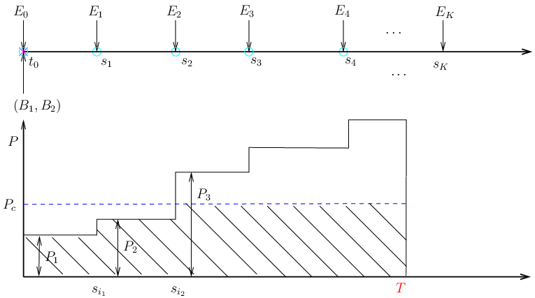
When , based on (20), if , we have . Starting from , remains a constant until an energy constraint becomes tight. Therefore, between any two consecutive epochs, when the energy constraints are tight, the power level remains constant. Similar arguments hold when . Thus, the corresponding power level is
| (25) |
where and are two consecutive epochs with tight energy constraint.
Finally, we need to determine the epochs when the energy constraint becomes tight. Another observation is that must monotonically increase in , as shown in Fig. 6. This is because both of these two curves monotonically increase, and the maximum value of these two curves should monotonically increase also. Therefore, based on the monotonicity of the transmit power, we conclude that
| (26) |
This completes the proof.
Since the power can be obtained directly irrespective of the values of , , the optimization problem in (10) is separable over each duration . Specifically, for , the local optimization becomes
| s.t. | (27) |
We relax the power constraint to be an inequality to make the constraint set convex. Thus, this becomes a convex optimization problem. This does not affect the solution since the objective function is always maximized on the boundary of its constraint set, i.e., the capacity region defined by the transmit power .
When , the solution to (27) can be expressed as
| (28) | ||||
| (29) |
In this scenario, all of the power is allocated to the first user.
When , we have
| (30) | ||||
| (31) |
In this scenario, a constant amount of power, , is allocated to the first user, and the remaining power is allocated to the second user.
When , we have
| (32) | ||||
| (33) |
In this scenario, all of the is allocated to the second user.
Let us define a constant power level as
| (34) |
Based on the solution of the local optimization problem in (27), we establish another important property of the optimal policy as follows.
Lemma 4
For fixed , , under the optimal power policy, there exists a constant cut-off power level, , for the first user. If the total power level is below this cut-off power level, then, all the power is allocated to the first user; if the total power level is higher than this level, then, all the power above this cut-off level is allocated to the second user.
In the proof of Lemma 3, we note that the optimal power monotonically increases in . Combining Lemma 3 and Lemma 4, we illustrate the structure of the optimal policy in Fig. 7. Moreover, the optimal way of splitting the power in each epoch is such that both users’ shares of the power monotonically increase in time. In particular, the second user’s share is monotonically increasing in time. Hence, the path followed in the plane is such that it changes direction to get closer to the second user’s departure axis as shown in Fig. 4. The dotted trajectory cannot be optimal, since the path does not get closer to the second user’s departure axis in the middle (second) power epoch.
Corollary 1
Under the optimal policy, the transmission rate for the first user, , is either a constant sequence (zero or a positive constant), or an increasing sequence. Moreover, before achieves its final constant value, ; and when becomes a constant, monotonically increases in .
Based on Lemma 3, we observe that for fixed , and , the optimal total power allocation is unique, i.e., does not depend on and . However, the way the total power is split between the two users depends on , . In fact, the cut-off power level varies depending on the value of . Therefore, for different values of , the optimal policy achieves different boundary points on the maximum departure region, and varying the value of traces the boundary of this region.
In this section, we characterized the maximum departure region for any given time . We proved that the optimal total transmit power is the same as in the single-user case, and there exists a cut-off power for splitting the total transmit power to both users. In the next section, we will use these structural properties to solve the transmission completion minimization problem.
IV Minimizing the Transmission Completion Time for a Given
In this section, our goal is to minimize the transmission completion time of both users for a given . The optimization problem can be formulated as
| s.t. | (35) | ||||
where is the number of energy arrival epochs (excluding ) over , and . Since depends on , the optimization problem in (35) is not a convex optimization problem in general. Therefore, we cannot solve it using standard convex optimization tools.
We first note that this is exactly the “dual” problem of maximizing the departure region for fixed . They are “dual” in the sense that, if the minimal transmission completion time for is , then must lie on the boundary of , and the transmission policy should be exactly the same for some . This is based on the fact the for any . Assume does not lie on the boundary of . Then, either cannot be achieved by or is strictly inside and hence can be achieved by . Therefore, if does not lie on the boundary of , then cannot be the minimum transmission completion time.
We have the following lemma.
Lemma 5
When , under the optimal policy, the transmissions to both users must be finished at the same time.
Proof: This lemma can be proved based on Corollary 1. If the transmission completion time for both users is not the same, then over the last duration, we transmit only to one of the users, while the transmission rate to the other user is zero. This contradicts with the monotonicity of the transmission rates for both users. Therefore, under the optimal policy, the transmitter must finish transmitting to both users at the same time.
This lemma is proved in [11] also, by using a different approach. The authors prove it in [11] mainly based on the convexity of the capacity region of the broadcast channel.
For fixed , let us denote the transmission completion time for the first and second user, by and , respectively. We note that and depend on the selection of the cut-off power level, . In particular, is monotonically decreasing in , and is monotonically increasing in . Based on Lemma 5, the problem of optimal selection of , can be viewed as solving a fixed point equation. In particular, must be chosen such that, the resulting equals . Therefore, we propose the following algorithm to solve the transmission completion time, , minimization problem. Our basic idea is to try to identify the cut-off power level in an efficient way.
Since the power allocation is similar to the single-user case (c.f. Lemma 3), our approach to find will be similar to the method in [1, 2]. First, we aim to identify , the first total transmit power starting from in the system. This is exactly the same as identification of in the corresponding single-user problem. For this, as in [1, 2], we treat the energy arrivals as if they have arrived at time , and obtain a lower bound for the transmission completion time as in [1, 2]. In order to do that, first, we compute the amount of energy required to finish by . This is equal to , denoted as . Then, we compare with . If is greater than , this implies that the transmitter can finish the transmission before with , and future energy arrivals are not needed. In this case, the minimum transmission completion time is the solution of the following equation
| (36) |
If is greater than , this implies that the final transmission completion time is greater than , and some of the future energy arrivals must be utilized to complete the transmission. We calculate the amount of energy required to finish by , , …, and denote them as , , …, and compare these with , …, until the first that becomes smaller than . We denote the corresponding time index as . Then, we assume that we can use to transmit at a constant rate. And, the corresponding transmission completion time is the solution of the following equation
| (37) |
We denote the solution to this equation as , and the corresponding power as . From our analysis, we know that the solution to this equation is the minimum possible transmission completion time we can achieve. Then, we check whether this constant power is feasible, when the actual energy arrival times are imposed. If it is feasible, it gives us the minimal transmission completion time; otherwise, we get by selecting the minimal slope according to (15). That is to say, we draw all of the lines from to the corner points of the energy arrival instances before , and choose the line with the smallest slope. We denote by the corresponding duration associated with . This is shown in Fig. 8.
Once is selected, we know that it is the optimal total transmit power in our broadcast channel problem. Next, we need to divide this total power between the signals transmitted to the two users. Based on Lemma 4 and Corollary 1, if the cut-off power level is higher than , then, the transmitter spends all for the stronger user; otherwise, the first user finishes its transmission with a constant power .
We will first determine whether lies in or it is higher than . Assume . Therefore, the transmission completion time for the first (stronger) user is
| (38) |
Once is fixed, we can obtain the minimum transmission completion time for the second user, , by subtracting the energy consumed by the first user, and treating as an interference for the second user. This reduces the problem to the single-user problem for the second user with fading, where the fading level is over , and afterwards. The single-user problem with fading is studied in [10]. Since obtaining the minimal transmission completion time is not as straightforward for the fading channel, a more approachable way is to calculate the maximum number of bits departed from the second user by , denoted as . In order to do that, we first identify the optimal power allocation policy with fixed deadline . This can be done according to Lemma 3. Assume that the optimal power allocation gives us . Then, we allocate to the first user over the whole duration, and allocate the remaining power to the second user. Based on (4), we calculate the transmission rate for the second user over each duration, and obtain according to
| (39) |
We observe that, given , is a monotonically increasing function of . Moreover, given , is a monotonically decreasing function of .
If is smaller than , it implies that , and we need to decrease the rate for the first user to make and equal. Based on Lemma 4, this also implies that the transmission power for the first user is a constant . In particular, is the unique solution of
| (40) |
Note that is a continuous, strictly monotonically decreasing function of , hence the solution for in (40) is unique. Since is a decreasing function of and is a decreasing function of , we can use the bisection method to solve (40). In this case, the minimum transmission completion time is .
If is larger than , that implies , and we need to increase the power allocated for the first user to make and equal, i.e., . Therefore, from Lemma 4, over the duration , the optimal policy is to allocate the entire to the first user only. We allocate to the first user, calculate the number of bits departed for the first user, and remove them from . This simply reduces the problem to that of transmitting bits starting at time , where . The process is illustrated in Fig. 9. Then, the minimum transmission completion time is
| (41) |
where is the number of recursions needed to get .
In both scenarios, we reduce the problem into a simple form, and obtain the final optimal policy. Before we proceed to prove the optimality of the algorithm, we introduce the following lemma first, which is useful in the proof of the optimality of the algorithm.
Lemma 6
monotonically increases in ; monotonically increases in also.
Proof: The monotonicity of both functions can be verified by taking derivatives,
| (42) |
and
| (43) |
where the inequality follows since . Therefore, is a strictly concave function, and its first derivative monotonically decreases when increases. Since when , when , we have , therefore, the monotonicity follows.
Similarly, we have
| (44) |
and
| (45) |
Again, the concavity implies that the first derivative is positive when , and the monotonicity follows.
Theorem 1
The algorithm is feasible and optimal.
Proof: We first prove the optimality. In order to prove that the algorithm is optimal, we need to prove that is optimal. Once we prove the optimality of , the optimality of , , follows. Since the solution obtained using our algorithm always has the optimal structure described in Lemma 4, the optimality of the power allocation also implies the optimality of the rate selection, thus, the optimality of the algorithm follows. Therefore, in the following, we prove that is optimal.
First, we note that is the minimal slope up to . We need to prove that is also the minimal slope up to the final transmission completion time, . Let us define as follows
| (46) |
Assume that with , we allocate to the first user, and finish using constant rates. Then, we allocate to the first user, and the rest to the second user. Based on Lemma 6, we have
| (47) | ||||
| (48) |
Therefore, is an upper bound for the optimal transmission completion time. Since is the minimal slope up to , we conclude that is optimal throughout the transmission. Following similar arguments, we can prove the optimality of the rest of the power allocations. This completes the proof of optimality.
In order to prove that the allocation is feasible, we need to show that the power allocation for the first user is always feasible in each step. Therefore, in the following, we first prove that is feasible when we assume that . The feasibility of also implies the feasibility of the rest of the power allocation. With the assumption that , the final transmission time for the first user is
| (49) |
Based on (47) and (48), we know that . Since is feasible up to , therefore, is feasible when we assume that . The feasibility of the rest of the power allocations follows in a similar way. This completes the feasibility part of the proof.
V Numerical Examples
We consider a band-limited AWGN broadcast channel, with bandwidth MHz and the noise power spectral density W/Hz. We assume that the path loss between the transmitter and the first receiver is about dB, and the path loss between the transmitter and the second user is about dB. Then, we have
| (50) | ||||
| (51) |
Therefore,
| (52) |
For the energy harvesting process, we assume that at times s, we have energy harvested with amounts mJ. We find the maximum departure region for s, and plot them in Fig. 10. We observe that the maximum departure region is convex for each value of , and as increases, the maximum departure region monotonically expands.
Then, we aim to minimize the transmission completion time with Mbits. Following our algorithm, we obtain the optimal transmission policy, which is shown in Fig. 11. We note that the powers change only potentially at instances when energy arrives (Lemma 1); power sequence is monotonically increasing and “majorized” over the whole transmission duration (Lemma 3). We also note that, for this case, the first user transmits at a constant rate, and the rate for the second user monotonically increases. The transmitter finishes its transmissions to both users by time s, and the last energy harvest at time s is not used.
Next, we consider the example when Mbits, we have the optimal transmission policy, as shown in Fig. 12. In this example, the cut-off power is greater than , and therefore, is allocated to the first user only over s, and after s, the first user keeps transmitting at a constant rate until all bits are transmitted. In this case, the transmission rates for both users monotonically increase. The transmitter finishes its transmissions by time s, and the last energy harvest is not used.
VI Conclusions
We investigated the transmission completion time minimization problem in an energy harvesting broadcast channel. We first analyzed the structural properties of the optimal transmission policy, and proved that the optimal total transmit power has the same structure as in the single-user channel. We also proved that there exists a cut-off power for the stronger user. If the optimal total transmit power is lower than this cut-off level, all power is allocated to the stronger user, and when the optimal total transmit power is greater than this cut-off level, all power above this level is allocated to the weaker user. Based on these structural properties of the optimal policy, we developed an iterative algorithm to obtain the globally optimal off-line transmission policy.
References
- [1] J. Yang and S. Ulukus, “Transmission completion time minimization in an energy harvesting system,” th Annual Conference on Information Sciences and Systems (CISS), March 2010.
- [2] ——, “Optimal packet scheduling in an energy harvesting communication system,” IEEE Transactions on Communications, submitted, June 2010. Also available at [arXiv:1010.1295].
- [3] E. Uysal-Biyikoglu, B. Prabhakar, and A. El Gamal, “Energy-efficient packet transmission over a wireless link,” IEEE/ACM Transactions on Networking, vol. 10, pp. 487–499, August 2002.
- [4] M. A. Zafer and E. Modiano, “A calculus approach to energy-efficient data transmission with quality of service constraints,” IEEE/ACM Transactions on Networking, vol. 17, pp. 898–911, June 2009.
- [5] ——, “Delay-constrained energy efficient data transmission over a wireless fading channel,” Information Theory and Applications Workshop, pp. 289–298, January 2007.
- [6] W. Chen, U. Mitra, and M. Neely, “Energy-efficient scheduling with individual delay constraints over a fading channel,” WiOpt, pp. 1–10, April 2007.
- [7] A. El Gamal, C. Nair, B. Prabhakar, E. Uysal-Biyikoglu, and S. Zahedi, “Energy-efficient scheduling of packet transmissions over wireless networks,” IEEE Infocom, vol. 3, pp. 1773–1782, November 2002.
- [8] E. Uysal-Biyikoglu and A. El Gamal, “On adaptive transmission for energy efficiency in wireless data networks,” IEEE Transactions on Information Theory, vol. 50, pp. 3081–3094, December 2004.
- [9] K. Tutuncuoglu and A. Yener, “Optimum transmission policies for battery limited energy harvesting systems,” submitted, September 2010. Also available at http://wcan.ee.psu.edu.
- [10] O. Ozel, K. Tutuncuoglu, J. Yang, S. Ulukus, and A. Yener, “Resource management for fading wireless channels with energy harvesting nodes,” submitted.
- [11] M. A. Antepli and E. Uysal-Biyikoglu, “Optimal packet scheduling on an energy harvesting broadcast link,” submitted.
- [12] T. M. Cover and J. A. Thomas, Elements of Information Theory. New York: John Wiley and Sons, Inc, 1991.