跳到论文正文
W Papers独立论文阅读器 arXiv:1010.2743 论文正文 计算阅读时间 · 0%
引用这篇论文根据当前论文元数据生成,正式投稿前建议核对。


License: arXiv.org perpetual non-exclusive license
arXiv:1010.2743v2 [hep-ph] 20 Jan 2011

IFUM-966-FT

MAN/HEP/2010/13

Small xx resummation of rapidity distributions:
the case of Higgs production

Fabrizio Caolaa, Stefano Fortea and Simone Marzanib

aDipartimento di Fisica, Università di Milano and INFN, Sezione di Milano,
Via Celoria 16, I-20133 Milano, Italy

bSchool of Physics & Astronomy, University of Manchester,
Oxford Road, Manchester, M13 9PL, England, U.K.

Abstract:

We provide a method for the all order computation of small xx contributions at the leading logarithmic level to cross-sections which are differential in rapidity. The method is based on a generalization to rapidity distributions of the high energy (or kTk_{T}) factorization theorem hitherto proven for inclusive cross-sections. We apply the method to Higgs production in gluon-gluon fusion, both with finite top mass and in the infinite mass limit: in both cases, we determine all-order resummed expressions, as well as explicit expressions for the leading small xx terms up to NNLO. We use our result to construct an explicit approximate analytic expression of the finite–mass NLO rapidity distribution and an estimate of finite–mass corrections at NNLO.

October 2010

1 Introduction

Techniques for the computation of small xx logarithmically enhanced contributions to hard QCD cross-sections to all orders have been available for some time, and have been successfully applied to a variety of hard processes: heavy quark photo- and lepto-production [1], Deep-Inelastic Scattering [2], and more recently hadroproduction processes, including heavy quarks [3], Higgs (both in the infinite top mass limit [4] and for finite mtopm_{\rm top}  [5, 6]), Drell-Yan [7] and prompt-photon [8]. In each of these cases, the leading contribution to the hard cross-section in the x→0x\to 0 limit has been determined to all orders in the strong coupling αs​(Q2)\alpha_{s}(Q^{2}), where Q2Q^{2} is the hard scale of the process (typically related to the invariant mass of the final state for hadroproduction processes), and xx is the dimensionless ratio of this scale to the available (partonic) center-of-mass energy x=Q2/sx=Q^{2}/s.

The interest in these results is twofold. First, they provide information on unknown higher–order contributions (or cross-checks on known ones): for example, the NNLO leading small xx contribution to Higgs production in the finite mtopm_{\rm top} case [5] was used in Ref. [9] to construct an approximate expression for the yet unknown full NNLO term by combining it with an expansion in 1/mtop1/m_{\rm top} [10, 11]. Second, they can be used to construct all order resummed results, which may be necessary in the kinematic region where αs​ln⁡1x∼1\alpha_{s}\ln{{1}\over{x}}\sim 1 so that the conventional perturbative expansion becomes unstable. For many processes mentioned above, such as Deep-Inelastic Scattering or Drell-Yan, the Born cross-section is a quark-induced O⁡(αs0)O(\alpha_{s}^{0}) electroweak process (parton model), so that the leading-log resummation of hard cross-sections is only consistent (i.e. resummed results are only factorization–scheme invariant) if combined with a next-to-leading log resummation of evolution equations. Such a consistent resummation is possible because not only leading [12] but also next-to-leading [13] ln⁡1x\ln{{1}\over{x}} contributions to evolution equations are known since some time, as well as methods to use resummed evolution equations in a way compatible with physical constraints [14, 15], and to combine solutions to resummed evolution equations with resummed hard partonic cross-sections [16, 17].

The usefulness of these results for phenomenology has been hampered so far by the fact that they, and the computational techniques on which they are based, are only available for fully inclusive cross-sections. This is likely to become a very serious limitation at the LHC where, for instance, the LHCb experiment will measure Drell-Yan rapidity distributions at very small invariant masses (i.e. at very small xx) but in a limited rapidity range [18]. It is the purpose of this paper to overcome this limitation by extending the resummation formalism to rapidity distributions.

Available calculations at small xx are based on a suitable formulation of QCD factorization which is consistent with all-order leading log xx resummation, called high energy or kTk_{T} factorization [1, 19]. Generalization of this factorization to the less inclusive case is a prerequisite for resummation, and it will be accomplished here. We will proceed as follows. First, in Sect. 2 we will rederive the standard high energy factorization for inclusive cross-sections of Refs. [1, 19]. This derivation is completely equivalent to that of Refs. [1, 19], but it differs from it because the ladder expansion which underlies the factorization is treated in a way which is “dual” to it in the sense of Ref. [20]: small xx logs are factored as part of standard DGLAP splitting functions, rather than by solving a BFKL [12] equation for the gluon Green function.

The consequence of this is that the same kinematic as in the proof of collinear factorization [21] can be used. Within this kinematics, the dependence on transverse and longitudinal momentum components are kept separate from each other, and this renders the generalization to rapidity distributions possible. This result is derived in Sect. 3, where a simple formula for the computation of leading log xx contributions to rapidity distributions to all orders is arrived at, in terms of the Fourier-Mellin transform of the partonic rapidity distribution computed at the lowest nontrivial order with incoming off-shell gluons.

In the second part of the paper we apply this formalism to Higgs production in gluon-gluon fusion. First, in Sect. 4 we summarize the small xx behavior of rapidity distributions in this case, both in the limit mtop→∞m_{\rm top}\to\infty and for finite top mass, and specifically we obtain explicit results for LLxx terms up to NNLO, already known at NLO in the mtop→∞m_{\rm top}\to\infty limit, but otherwise determined here for the first time in closed form. In Sect. 5 we then apply to this case the resummation formula of Sect. 3, by deriving a resummed expression and explicit coefficients up to NNLO. We check that the results up to O⁡(αs4)O(\alpha_{s}^{4}) of the previous section are reproduced (which turns out to happen in a rather nontrivial way), we construct an explicit analytic matched O⁡(αs3)O(\alpha_{s}^{3}) expression in the finite mtopm_{\rm top} case, and compare it to known numerical results [26, 27]. We also give an estimate of finite mass corrections at NNLO. Technical results on MS¯\overline{\textsc{MS}} factorization and subtraction of collinear singularities both at the inclusive and differential level are collected in two appendices.

2 High energy factorization of inclusive cross - sections

We will rederive high energy factorization [1, 19] in the leading logarithmic approximation (LLxx) for inclusive quantities. After some introductory comments, we will first consider the known case of nn-gluon emission at the double log (i.e. LLxx-LLQ2Q^{2}) level, and finally the nontrivial general LLxx case. We then recall how the factorized result can be exploited for resummation, and finally we compare directly our approach to the original one of Refs. [1, 19]. The key idea of our argument is to exploit the factorization of the partonic cross-section in terms of a hard part and a ladder part, but then compute the ladder part using standard collinear factorization and DGLAP evolution, rather than BFKL evolution, exploiting the fact that due to perturbative duality [20, 28] they are in fact equivalent at the leading twist level.

2.1 Factorized cross-section

In order to simplify our derivation, we consider at first a photo- or lepto-production process

𝒱⁡(n)+g⁡(p)→𝒮+X.{\cal V}(n)+g(p)\rightarrow\mathcal{S}+X. (1)

characterized by a hard scale Q2Q^{2}. In Eq. (1) g⁡(p)g(p) denotes a gluon of momentum pp, 𝒱⁡(n){\cal V}(n) denotes an electroweak gauge boson of momentum nn, not necessarily on-shell: e.g. for neutral-current Deep-Inelastic Scattering 𝒱=γ∗{\cal V}=\gamma^{*} or 𝒱=Z∗{\cal V}=Z^{*}, and 𝒮\mathcal{S} the desired final state (a quark for DIS, a dilepton for Drell-Yan and so forth). Generalization to hadroproduction or quark-initiated processes is straightforward and will be discussed In Sect. 2.6.

Our starting point is the same of Refs. [1, 19], namely the observation [12, 29] that in an axial gauge high energy enhanced terms only come from cut diagrams which are at least two-gluon reducible in the tt-channel (see Fig. 1). The generic dimensionless partonic cross-section σ\sigma can then be split in a (process-dependent) two-gluon irreducible part (“hard” part), and a generally two-gluon reducible part (“ladder” part):

σ=∫Q22​s​Hμ​ν​(n,pL,pℱ,μR,μF,αs)⋅Lμ​ν​(pL,p,μR,μF,αs)​[d​pL],\sigma=\int{{Q^{2}}\over{2s}}H^{\mu\nu}(n,p_{L},p_{\mathcal{F}},\mu_{R},\mu_{F},\alpha_{s})\cdot L_{\mu\nu}(p_{L},p,\mu_{R},\mu_{F},\alpha_{s})\left[{d}p_{L}\right], (2)

where the hard part Hμ​νH^{\mu\nu} includes the phase space for the observed final state 𝒮\mathcal{S} and the momentum conservation delta function and we have also made explicit the flux factor 1/(2​s)1/(2s). Here pℱp_{\mathcal{F}} stands for a set of momenta parametrizing the final state of the hard part, which we will henceforth denote as ℱ\mathcal{F}, see Fig. 2. The measure [d​pL]\left[{d}p_{L}\right] is the pLp_{L}–loop integration measure for the cut diagram Fig. 1 and will be specified in the following (see Eq. (7) below).

Diagrams like Fig. 1 contain in general both ultraviolet and infrared divergences, which must be regulated. This leads to the dependence of the partonic cross-section on the renormalization μR\mu_{R} and factorization μF\mu_{F} scales. The renormalization scale dependence can be reabsorbed in the running coupling αs​(μR)\alpha_{s}(\mu_{R}). Since running coupling effects are NLLxx, while we are working at the LLxx level, in the following we will omit all the μR\mu_{R} dependence and consider only the dependence on μF\mu_{F}, which from now on we will call just μ\mu.

In order to simplify our derivation, we will assume further that the hard part is not just 2-gluon irreducible (2GI), but in fact 2-particle irreducible (2PI). This implies that we can neglect the μF=μ\mu_{F}=\mu dependence in Hμ​νH^{\mu\nu}. The generalization to the case in which the hard part is 2GI but two-particle reducible has been worked out in [2]; the extension of our formalism to it would be straightforward but we will not discuss it further. The functions Hμ​νH^{\mu\nu} and Lμ​νL^{\mu\nu} thus depend on the following variables:

Hμ​ν=Hμ​ν​(n,pL,pℱ,αs)\displaystyle H^{\mu\nu}=H^{\mu\nu}(n,p_{L},p_{\mathcal{F}},\alpha_{s})
Lμ​ν=Lμ​ν​(pL,p,μ,αs)\displaystyle L^{\mu\nu}=L^{\mu\nu}(p_{L},p,\mu,\alpha_{s}) (3)
Refer to caption
Figure 1: Left: decomposition of the cut partonic cross-section in terms of two-gluon irreducible hard part and a reducible ladder part. Right: generalized ladder expansion of the ladder part.

Since everything is on-shell and we are working in an axial gauge, we can decompose both the hard part and the ladder part in terms of conserved Lorentz structures time dimensionless scalar functions:

Hμ​ν​(n,pL,pℱ,αs)=(−gμ​ν+pLμ​pLνpL2)​H⟂​(Q2n⋅pL,−pL2Q2,Ωℱ,αs)+\displaystyle H^{\mu\nu}(n,p_{L},p_{\mathcal{F}},\alpha_{s})=\left(-g^{\mu\nu}+{{p_{L}^{\mu}p_{L}^{\nu}}\over{p_{L}^{2}}}\right)H_{\perp}\left({{Q^{2}}\over{n\cdot p_{L}}},{{-p_{L}^{2}}\over{Q^{2}}},\Omega_{\mathcal{F}},\alpha_{s}\right)+
+pL2​(pLμpL2−nμn⋅pL)​(pLνpL2−nνn⋅pL)​H|⁣|​(Q2n⋅pL,−pL2Q2,Ωℱ,αs)\displaystyle+p_{L}^{2}\left({{p_{L}^{\mu}}\over{p_{L}^{2}}}-{{n^{\mu}}\over{n\cdot p_{L}}}\right)\left({{p_{L}^{\nu}}\over{p_{L}^{2}}}-{{n^{\nu}}\over{n\cdot p_{L}}}\right)H_{||}\left({{Q^{2}}\over{n\cdot p_{L}}},{{-p_{L}^{2}}\over{Q^{2}}},\Omega_{\mathcal{F}},\alpha_{s}\right) (4)
Lμ​ν​(pL,p,μ,αs)=1pL2​(−gμ​ν+pLμ​pLνpL2)​L⟂​(−pL2p⋅pL,μ2−pL2,αs)\displaystyle L^{\mu\nu}(p_{L},p,\mu,\alpha_{s})={{1}\over{p_{L}^{2}}}\left(-g^{\mu\nu}+{{p_{L}^{\mu}p_{L}^{\nu}}\over{p_{L}^{2}}}\right)L_{\perp}\left({{-p_{L}^{2}}\over{p\cdot p_{L}}},{{\mu^{2}}\over{-p_{L}^{2}}},\alpha_{s}\right)
+(pLμpL2−pμp⋅pL)​(pLνpL2−pνp⋅pL)​L|⁣|​(−pL2p⋅pL,μ2−pL2,αs)\displaystyle+\left({{p_{L}^{\mu}}\over{p_{L}^{2}}}-{{p^{\mu}}\over{p\cdot p_{L}}}\right)\left({{p_{L}^{\nu}}\over{p_{L}^{2}}}-{{p^{\nu}}\over{p\cdot p_{L}}}\right)L_{||}\left({{-p_{L}^{2}}\over{p\cdot p_{L}}},{{\mu^{2}}\over{-p_{L}^{2}}},\alpha_{s}\right) (5)

where Ωℱ\Omega_{\mathcal{F}} stands for a set of (typically angular, see e.g. [7]) dimensionless variables which characterize the final state ℱ\mathcal{F}. Note that we have explicitly extracted the propagator factor 1/pL21/p_{L}^{2} from the scalar functions L||,⟂L_{||,\perp}.

In the high energy limit Eq. (2) simplifies somewhat. To see this, we work in the center-of-mass frame of the colliding partons and introduce the Sudakov parametrization

pL=z​p−k−kT2s⁡(1−z)​n=(s2​z,−kT22​s​(1−z),−𝐤T)p_{L}=zp-k-{{k_{T}^{2}}\over{s(1-z)}}n=\left(\sqrt{{{s}\over{2}}}z,-{{k_{T}^{2}}\over{\sqrt{2s}(1-z)}};-{\bf k}_{T}\right) (6)

where k=(0,kx,ky,0)k=(0,k_{x},k_{y},0) is a purely transverse four-vector with k2=−kT2<0k^{2}=-k_{T}^{2}<0 and as usual s=2​p⋅ns=2p\cdot n, and in the last step we have written the corresponding light-cone components. With this parametrization it is possible to show that the integration measure [d​pL]\left[dp_{L}\right] for the cut diagram Fig. 1 is (see e.g. [21])

[d​pL]=d​z2​(1−z)​d2​𝐤𝐓.\left[{d}p_{L}\right]={{{d}z}\over{2(1-z)}}{d}^{2}{\bf{k_{T}}}. (7)

Since the zz integration goes from xx to 1, we can easily identify the leading small xx region with the z≪1z\ll 1 region. As for kT2k_{T}^{2}, it is typically bounded by the hard scale Q2Q^{2}. Since in the high energy regime Q2≪sQ^{2}\ll s, we have kT2/s≪1k_{T}^{2}/s\ll 1. Summarizing, at small xx we are in the regime

z≪1;kT2s≪1;z\ll 1;\qquad{{k_{T}^{2}}\over{s}}\ll 1; (8)

subleading terms in zz and kT2/sk_{T}^{2}/s upon integration lead to power-suppressed O⁡(x)O(x) terms.

This kinematics leads to a simplification in the arguments of the scalar functions H||,⟂,L||,⟂H_{||,\perp},~L_{||,\perp}. We have

H||,⟂(Q2n⋅pL,−pL2Q2,Ωℱ,αs)\displaystyle H_{||,\perp}\left({{Q^{2}}\over{n\cdot p_{L}}},{{-p_{L}^{2}}\over{Q^{2}}},\Omega_{\mathcal{F}},\alpha_{s}\right) =\displaystyle= H||,⟂(Q2z​s,kT2Q2​(1−z),Ωℱ,αs)\displaystyle H_{||,\perp}\left({{Q^{2}}\over{zs}},{{k_{T}^{2}}\over{Q^{2}(1-z)}},\Omega_{\mathcal{F}},\alpha_{s}\right)
=\displaystyle= H||,⟂(Q2z​s,kT2Q2,Ωℱ,αs)(1+O(z))\displaystyle H_{||,\perp}\left({{Q^{2}}\over{zs}},{{k_{T}^{2}}\over{Q^{2}}},\Omega_{\mathcal{F}},\alpha_{s}\right)(1+O(z))
L||,⟂(−pL2p⋅pL,μ2−pL2,αs)\displaystyle L_{||,\perp}\left({{-p_{L}^{2}}\over{p\cdot p_{L}}},{{\mu^{2}}\over{-p_{L}^{2}}},\alpha_{s}\right) =\displaystyle= L||,⟂(−12,μ2kT2,αs)(1+O(z))\displaystyle L_{||,\perp}\left(-{{1}\over{2}},{{\mu^{2}}\over{k_{T}^{2}}},\alpha_{s}\right)(1+O(z)) (9)
=\displaystyle= L||,⟂(μ2kT2,αs)(1+O(z)).\displaystyle L_{||,\perp}\left({{\mu^{2}}\over{k_{T}^{2}}},\alpha_{s}\right)(1+O(z)).

With this in mind, and using the fact [1] that the scalar functions H⟂H_{\perp} and H|⁣|H_{||} have the same small xx behavior, and similarly L⟂L_{\perp} and L|⁣|L_{||}, we can write the differential dimensionless cross-section as

d​σ=−Q22​s​[2z2​H|⁣|​(Q2z​s,kT2Q2,Ωℱ,αs)​L|⁣|​(μ2kT2,αs)​(1+O⁡(z))]​d​z​d2​𝕜TkT2=\displaystyle{d}\sigma=-{{Q^{2}}\over{2s}}\left[{{2}\over{z^{2}}}H_{||}\left({{Q^{2}}\over{zs}},{{k_{T}^{2}}\over{Q^{2}}},\Omega_{\mathcal{F}},\alpha_{s}\right)L_{||}\left({{\mu^{2}}\over{k_{T}^{2}}},\alpha_{s}\right)\left(1+O(z)\right)\right]{d}z{{{d}^{2}\mathbb{k}_{T}}\over{k_{T}^{2}}}=
=[−Q22​s​z​H|⁣|​(Q2z​s,kT2Q2,Ωℱ,αs)​(1+O⁡(z))]​[2​π​L|⁣|​(μ2kT2,αs)]​d​zz​d​kT2kT2​d​θ2​π.\displaystyle=\left[-{{Q^{2}}\over{2sz}}H_{||}\left({{Q^{2}}\over{zs}},{{k_{T}^{2}}\over{Q^{2}}},\Omega_{\mathcal{F}},\alpha_{s}\right)\left(1+O(z)\right)\right]\left[2\pi L_{||}\left({{\mu^{2}}\over{k_{T}^{2}}},\alpha_{s}\right)\right]{{{d}z}\over{z}}{{{d}k_{T}^{2}}\over{k_{T}^{2}}}{{{d}\theta}\over{2\pi}}.

In Ref. [1] the ladder part Lμ​ν​(pL,p,μ,αs)L_{\mu\nu}(p_{L},p,\mu,\alpha_{s}) is computed at the LLxx level in terms of a gluon Green function, which in turns sums leading logs of xx by iterating a BFKL [12] kernel. Here we observe that we may equivalently express Lμ​ν​(pL,p,μ,αs)L_{\mu\nu}(p_{L},p,\mu,\alpha_{s}) in terms of the generalized ladder expansion of Ref. [21], and we will thus express it in terms of standard collinear anomalous dimensions. First, however, we discuss the hard part.

2.2 Hard part

Refer to caption
Figure 2: Graphic representation of the hard part in Eq. (2). Note that the hard part contains the momentum conservation delta function as well as the 𝒮\mathcal{S} and X~\tilde{X} phase space integration, but it does not contain phase space integration for gluons emitted along the ladder.

Let us now concentrate on the process-dependent hard part. We introduce a hard coefficient function CC defined as

C⁡(Q2z​s,Q2kT2,αs)≡∫02​πd​θ2​π​Q22​s​z​[𝒫μ​ν​Hμ​ν​(n,pL,pℱ,αs)]=\displaystyle C\left({{Q^{2}}\over{zs}},{{Q^{2}}\over{k_{T}^{2}}},\alpha_{s}\right)\equiv\int_{0}^{2\pi}{{{d}\theta}\over{2\pi}}{{Q^{2}}\over{2sz}}\left[\mathcal{P}_{\mu\nu}H^{\mu\nu}(n,p_{L},p_{\mathcal{F}},\alpha_{s})\right]=
=−∫02​πd​θ2​πQ22​s​zH|⁣|(Q2z​s,Q2kT2,Ωℱ,αs)(1+O(z)),\displaystyle=-\int_{0}^{2\pi}{{{d}\theta}\over{2\pi}}{{Q^{2}}\over{2sz}}H_{||}\left({{Q^{2}}\over{zs}},{{Q^{2}}\over{k_{T}^{2}}},\Omega_{\mathcal{F}},\alpha_{s}\right)\left(1+O(z)\right), (11)

where we have defined the projector

𝒫μ​ν≡kμ​kνkT2\mathcal{P}^{\mu\nu}\equiv{{k^{\mu}k^{\nu}}\over{k_{T}^{2}}} (12)

which, up to O⁡(z)O(z) terms, selects the longitudinal part H|⁣|H_{||} of the full Hμ​νH^{\mu\nu}. In Eq. (11) the explicit dependence of CC on Ωℱ\Omega_{\mathcal{F}} is understood.

Equation (11) has a simple interpretation: CC is the cross-section for the partonic process 𝒱⁡(n)+g∗​(q)→ℱ{\cal V}(n)+g^{*}(q)\rightarrow\mathcal{F} for an off-shell incoming gluon with momentum

q=z​p+k;q2=−kT2.q=zp+k;\quad q^{2}=-k_{T}^{2}. (13)

In this interpretation, 𝒫\mathcal{P} can be thought of as the sum over the polarizations of the off-shell gluon. Note that

⟨𝒫μ​ν⟩θ≡∫02​πd​θ2​π​𝒫μ​ν=12​(−gμ​ν+qμ​nν+qν​nμq⋅n)≡dμ​ν2,\left<\mathcal{P}^{\mu\nu}\right>_{\theta}\equiv\int_{0}^{2\pi}{{d\theta}\over{2\pi}}\mathcal{P}^{\mu\nu}={{1}\over{2}}\left(-g_{\mu\nu}+{{q_{\mu}n_{\nu}+q_{\nu}n_{\mu}}\over{q\cdot n}}\right)\equiv{{d_{\mu\nu}}\over{2}}, (14)

i.e. the azimuthal average of 𝒫μ​ν\mathcal{P}^{\mu\nu} performs the average over the polarizations of an on-shell gluon with momentum qq. Equations (11, 14) then imply

limkT2→0⟨C(Q2z​s,Q2kT2,αs)⟩θ=σon-shell(𝒱(n),g(zp)→ℱ),\lim_{k_{T}^{2}\rightarrow 0}\left<C\left({{Q^{2}}\over{zs}},{{Q^{2}}\over{k_{T}^{2}}},\alpha_{s}\right)\right>_{\theta}=\sigma_{\text{on-shell}}\left({\cal V}(n),g(zp)\rightarrow\mathcal{F}\right), (15)

i.e. in the limit kT/Q2→0k_{T}/Q^{2}\rightarrow 0 the azimuthal average of the hard coefficient function CC reduces to the on-shell partonic (dimensionless) cross-section. Note that in high energy kinematics Eq. (8), unlike in standard collinear kinematics, we cannot assume kT2≪Q2k_{T}^{2}\ll Q^{2} and thus the full dependence on kT2Q2{{k_{T}^{2}}\over{Q^{2}}} must be retained in the coefficient function CC Eq. (11). However, the assumption that kT2≪sk_{T}^{2}\ll s is sufficient [1] for the factorization of the cross-section Eq. (2) to hold.

For the subsequent discussion, it is important to observe that in the limit x→0x\to 0 the hard part, being 2GI, is finite, i.e. it does not contain logarithmically enhanced contributions. In particular, unless the vertex of the interaction for the process 𝒱⁡(n)+g∗​(q)→ℱ{\cal V}(n)+g^{*}(q)\rightarrow\mathcal{F} is pointlike, [1]

limx→0C⁡(x,Q2kT2,αs)=0.\lim_{x\to 0}C\left(x,{{Q^{2}}\over{k_{T}^{2}}},\alpha_{s}\right)=0. (16)

This is for instance the case for Deep-Inelastic Scattering and for heavy quark, Drell-Yan or Higgs production with finite mtopm_{\rm top}. For Higgs production in the mtop→∞m_{\rm top}\to\infty limit the effective gluon-gluon-Higgs interaction is pointlike, and in such a case [4]

limx→0C⁡(x,Q2kT2,αs)=C0\lim_{x\to 0}C\left(x,{{Q^{2}}\over{k_{T}^{2}}},\alpha_{s}\right)=C_{0} (17)

with C0C_{0} some constant. As it is well known, and as we will see explicitly in Sect. 4 the behavior Eq. (17) leads to double logarithmic small xx singularities.

2.3 Ladder part: generalities and double log approximation

We now turn to the computation of the ladder part. Unlike the hard part, which is 2PI, the ladder part may contain collinear singularities. In general, the collinear singularities of the partonic cross-section σ\sigma, Eq. (2), originate from those of the ladder part, and from the collinear region of the integration of the momentum pLp_{L} which connects the hard and ladder part. Collinear singularities can be subtracted from the partonic cross-section and factored in the parton distributions, to which the hard cross-section is connected by the lower line with momentum pp, using the iterative procedure of Ref. [21], based on a generalized ladder expansion. As already mentioned, after regularization and factorization of the collinear singularities the ladder part is a function of kT2μ2{{k_{T}^{2}}\over{\mu^{2}}}, where μ\mu is the (factorization) scale introduced in the course of regularization.

In the generalized ladder expansion, L|⁣|L_{||} is written as a sum of terms each of which, after regularization and factorization, leads to a contribution proportional to lnn⁡kT2μ2\ln^{n}{{k_{T}^{2}}\over{\mu^{2}}} to the cross-section, with nn ranging from one to infinity. The nn-th order contribution comes from a ladder diagram obtained iterating nn times a kernel K⁡(pi,pi−1,μ,αs)K(p_{i},p_{i-1},\mu,\alpha_{s}) with i=1,2,…,ni=1,2,\dots,n. To simplify our notation, from now on we will make the identifications pn≡pLp_{n}\equiv p_{L}, p0≡pp_{0}\equiv p, see Fig. 1. Subsequent iterations of the kernel are connected by a pair of tt-channel lines with momenta pnp_{n} (see Fig. 1) and ordered transverse momenta kT, 12≪kT, 22≪⋯≪kT,n2=kT2k^{2}_{T,\,1}\ll k^{2}_{T,\,2}\ll\dots\ll k^{2}_{T,\,n}=k^{2}_{T}. Because we are interested in the high energy limit, reducible lines are all gluon lines: quark contributions only appear at NLLxx and subsequent orders [1]. While we refer to Ref. [21] for a detailed discussion, the way the factorization of collinear singularities is performed in the generalized ladder expansion is summarized in Appendix A.

We will now show how to compute the ladder part using the generalized ladder expansion in the double logarithmic approximation, i.e. in the very simple case in which the result is determined simultaneously at the LLxx and LLQ2Q^{2}, and then turn in Sect. 2.4 to the more general LLxx case which we are interested in. At LLxx-LLQ2Q^{2}, the kernel K⁡(pi,pi−1,μ,αs)K(p_{i},p_{i-1},\mu,\alpha_{s}) must be linear in αs\alpha_{s} because the highest power of lnn⁡kT2μ2\ln^{n}{{k_{T}^{2}}\over{\mu^{2}}} in the cross-section must coincide with the order in αs\alpha_{s}. We define thus

K1​(μ2kT2,αs)≡K|⁣|LL​Q2​(μ2kT2,αs)K^{1}\left({{\mu^{2}}\over{k_{T}^{2}}},\alpha_{s}\right)\equiv K^{{\rm LL}Q^{2}}_{||}\left({{\mu^{2}}\over{k_{T}^{2}}},\alpha_{s}\right) (18)

with K1K^{1} linear in αs\alpha_{s}.

Consider first the case in which the kernel K1K^{1} is only inserted once. The corresponding (integrated) contribution to the cross-section Eq. (2.1) is given by

σ¯1​(Q2s,μ2Q2,αs)=∫x1d​zz​∫d​kT2kT2​C​(Q2z​s,Q2kT2,αs)​[2​π​K1​(μ2kT2,αs)],\bar{\sigma}^{1}\left({{Q^{2}}\over{s}},{{\mu^{2}}\over{Q^{2}}},\alpha_{s}\right)=\int_{x}^{1}{{{d}z}\over{z}}\int{{{d}k_{T}^{2}}\over{k_{T}^{2}}}C\left({{Q^{2}}\over{zs}},{{Q^{2}}\over{k_{T}^{2}}},\alpha_{s}\right)\left[2\pi K^{1}\left({{\mu^{2}}\over{k_{T}^{2}}},\alpha_{s}\right)\right], (19)

where the bar over σ\sigma indicates that collinear singularities have still to be subtracted from the cross-section, so this expression only makes sense at a regularized level. It is convenient to introduce the dimensionless variables

x≡Q2s;ξ≡kT2Q2,x\equiv{{Q^{2}}\over{s}};\qquad\xi\equiv{{k_{T}^{2}}\over{Q^{2}}}, (20)

in terms of which Eq. (19) becomes

σ¯1​(x,μ2Q2,αs)=∫x1d​zz​∫d​ξξ​C​(xz,ξ,αs)​[2​π​K1​(μ2Q2​ξ,αs)].\bar{\sigma}^{1}\left(x,{{\mu^{2}}\over{Q^{2}}},\alpha_{s}\right)=\int_{x}^{1}{{{d}z}\over{z}}\int{{{d}\xi}\over{\xi}}C\left({{x}\over{z}},\xi,\alpha_{s}\right)\left[2\pi K^{1}\left({{\mu^{2}}\over{Q^{2}\xi}},\alpha_{s}\right)\right]. (21)

Note that in terms of these variables

μ2Q2​ξ=μ2kT2,{{\mu^{2}}\over{Q^{2}\xi}}={{\mu^{2}}\over{k_{T}^{2}}}, (22)

i.e. the combination Q2​ξ/μ2Q^{2}\xi/\mu^{2} is Q2Q^{2} independent, and a lnn⁡kT2μ2\ln^{n}{{k_{T}^{2}}\over{\mu^{2}}} term shows up as lnn⁡Q2​ξμ2\ln^{n}{{Q^{2}\xi}\over{\mu^{2}}}.

The zz convolution in Eq. (21) is turned into an ordinary product by Mellin transformation:

f⁡(N)≡∫01d​x​xN−1​f​(x);f⁡(x)=∫c−i​∞c+i​∞d​N2​π​i​x−N​f​(N)f(N)\equiv\int_{0}^{1}{d}xx^{N-1}f(x);\qquad f(x)=\int_{c-i\infty}^{c+i\infty}{{{d}N}\over{2\pi i}}x^{-N}f(N) (23)

(note that by slight abuse of notation we denote with the same letter both the function and its transform). We get

σ¯1​(N,μ2Q2,αs)=∫d​ξξ​C​(N,ξ,αs)​[2​πN​K1​(μ2Q2​ξ,αs)].\bar{\sigma}^{1}\left(N,{{\mu^{2}}\over{Q^{2}}},\alpha_{s}\right)=\int{{{d}\xi}\over{\xi}}C\left(N,\xi,\alpha_{s}\right)\left[{{2\pi}\over{N}}K^{1}\left({{\mu^{2}}\over{Q^{2}\xi}},\alpha_{s}\right)\right]. (24)

Since in the limit ξ→0\xi\to 0 (i.e. kT2→0k_{T}^{2}\rightarrow 0 ) the coefficient function CC does not vanish (see Eq. (15)), Eq. (24) is collinear divergent. We use dimensional regularization and let d=4−2​ϵd=4-2\epsilon. It can be shown [2] that in dd dimensions 𝒫μ​ν\mathcal{P}^{\mu\nu} is still given by Eq. (12), hence Eq. (15) remains true also in d=4−2​ϵd=4-2\epsilon dimensions.

The regularized expression is explicitly given by11 1 Henceforth, to simplify notation we omit terms like (4​π)ϵ/Γ⁡(1−ϵ)(4\pi)^{\epsilon}/\Gamma(1-\epsilon), which in the MS¯\overline{\textsc{MS}} scheme are subtracted anyway. Full details on the calculation are given in Appendix A.:

σ¯1​(N,μ2Q2,αs,ϵ)​∫0∞d​ξξ1+ϵ​C​(N,ξ,αs,ϵ)​[2​πN​K1​((μ2Q2)ϵ​αs,N,ϵ)],\bar{\sigma}^{1}\left(N,{{\mu^{2}}\over{Q^{2}}},\alpha_{s};\epsilon\right)\int_{0}^{\infty}{{d\xi}\over{\xi^{1+\epsilon}}}C\left(N,\xi,\alpha_{s};\epsilon\right)\left[{{2\pi}\over{N}}K^{1}\left(\left({{\mu^{2}}\over{Q^{2}}}\right)^{\epsilon}\alpha_{s};N,\epsilon\right)\right], (25)

where the dependence of K1K^{1} on NN is O⁡(ϵ)O(\epsilon). In Eq. (25) the limit ξ→∞\xi\rightarrow\infty is never reached, because kT2k_{T}^{2} is bounded by the kinematics (typically kT2<Q2k_{T}^{2}<Q^{2}). Note that we have used the assumption that the hard part is 2PI, which ensures that CC is free of collinear singularities [21, 30]. The generalization to processes for which HH is 2GI but not 2PI (such as Deep-Inelastic Scattering and Drell-Yan) requires also treating the collinear singularities in HH [2, 7]. Note that the dependence on μ2\mu^{2} enters only through the combination (μ2)ϵ​αs(\mu^{2})^{\epsilon}\alpha_{s} and it is thus fixed by dimensional analysis.

Using the expansion

1ξ1+ϵ=−δ⁡(ξ)ϵ+∑i=0∞[lni⁡ξξ]+​(−ϵ)ii!{{1}\over{\xi^{1+\epsilon}}}=-{{\delta(\xi)}\over{\epsilon}}+\sum_{i=0}^{\infty}\left[{{\ln^{i}\xi}\over{\xi}}\right]_{+}{{(-\epsilon)^{i}}\over{i!}} (26)

in Eq. (25) we get

σ¯1(N,μ2Q2,αs;ϵ)=−1ϵσon-shell×[2​πNK1(αs)]+finite,\bar{\sigma}^{1}\left(N,{{\mu^{2}}\over{Q^{2}}},\alpha_{s};\epsilon\right)=-{{1}\over{\epsilon}}\sigma_{\text{on-shell}}\times\left[{{2\pi}\over{N}}K^{1}\left(\alpha_{s}\right)\right]+\text{finite}, (27)

where σon-shell\sigma_{\text{on-shell}} is the on-shell cross-section for the process 𝒱⁡(n)+g⁡(z​p)→ℱ{\cal V}(n)+g(zp)\rightarrow\mathcal{F}, see Eq. (15). Equation (27) shows that 2​π​K1​(αs)/N2\pi K^{1}(\alpha_{s})/N is the residue of the O⁡(αs)O(\alpha_{s}) collinear pole, i.e. the leading–order anomalous dimension. Because all the computation has been performed at the LLxx level, only the leading small xx contribution to the anomalous dimension is significant, so

2​πN​K1​(αs)=α¯s​γ0​(N);α¯s≡αs​Ncπ\displaystyle{{2\pi}\over{N}}K^{1}(\alpha_{s})=\bar{\alpha}_{s}\gamma_{0}(N);\qquad\bar{\alpha}_{s}\equiv{{\alpha_{s}N_{c}}\over{\pi}}
γ0​(N)=1/N.\displaystyle\qquad\gamma_{0}(N)=1/N. (28)

Having determined K1K^{1}, we can substitute it in Eq. (25):

σ¯1​(N,μ2Q2,αs,ϵ)=∫0∞d​ξξ1+ϵ​C​(N,ξ,αs,ϵ)​α¯s​(μ2Q2)ϵ​γ0​(N),\bar{\sigma}^{1}\left(N,{{\mu^{2}}\over{Q^{2}}},\alpha_{s};\epsilon\right)=\int_{0}^{\infty}{{d\xi}\over{\xi^{1+\epsilon}}}C\left(N,\xi,\alpha_{s};\epsilon\right)\bar{\alpha}_{s}\left({{\mu^{2}}\over{Q^{2}}}\right)^{\epsilon}\gamma_{0}(N), (29)

where we used the fact that the LO gluon-gluon anomalous dimension is ϵ\epsilon independent. Equation (29) is the expression for the regularized (collinear singular) cross-section 𝒱⁡(n)+g⁡(p)→ℱ+g{\cal V}(n)+g(p)\rightarrow\mathcal{F}+g in the small xx limit.

We are now ready to compute the ladder expansion of LL at LLxx, LLQ2Q^{2}. The regularized contribution to the cross-section when the kernel is iterated nn times is

σ¯n(N,μ2Q2,αs;ϵ)=[α¯s(μ2Q2)ϵγ0(N)]∫0∞d​ξnξn1+ϵC(N,ξn,αs;ϵ)×\displaystyle\bar{\sigma}^{n}\left(N,{{\mu^{2}}\over{Q^{2}}},\alpha_{s};\epsilon\right)=\left[\bar{\alpha}_{s}\left({{\mu^{2}}\over{Q^{2}}}\right)^{\epsilon}\gamma_{0}(N)\right]\int_{0}^{\infty}{{d\xi_{n}}\over{\xi_{n}^{1+\epsilon}}}C\left(N,\xi_{n},\alpha_{s};\epsilon\right)\times
×∫0ξn[α¯s​(μ2Q2)ϵ​γ0​(N)]​d​ξn−1ξn−11+ϵ×…×∫0ξ2[α¯s​(μ2Q2)ϵ​γ0​(N)]​d​ξ1ξ11+ϵ.\displaystyle\times\int_{0}^{\xi_{n}}\left[\bar{\alpha}_{s}\left({{\mu^{2}}\over{Q^{2}}}\right)^{\epsilon}\gamma_{0}(N)\right]{{d\xi_{n-1}}\over{\xi_{n-1}^{1+\epsilon}}}\times...\times\int_{0}^{\xi_{2}}\left[\bar{\alpha}_{s}\left({{\mu^{2}}\over{Q^{2}}}\right)^{\epsilon}\gamma_{0}(N)\right]{{d\xi_{1}}\over{\xi_{1}^{1+\epsilon}}}. (30)

Had we used a collinear cutoff μF\mu_{F} instead of dimensional regularization, the ordered integrations in Eq. (30) would give rise to the expected lnn⁡Q2/μF2\ln^{n}Q^{2}/\mu_{F}^{2} term. In dimensional regularization, Eq. (30) contains collinear ϵ\epsilon poles. Their MS¯\overline{\textsc{MS}} factorization using the generalized ladder expansion of Ref. [21] is performed by requiring Eq. (30) to be finite after each ξi\xi_{i} integration. This is done subtracting iteratively in such a way that Eq. (30) is finite also at the integrand level; details are given in Appendix A. This then leaves a single nn-th order ϵ\epsilon pole in the cross-section, which can be subtracted using standard MS¯\overline{\textsc{MS}}.

The result after iterative subtraction of the first n−1n-1 singularities is

σn(N,μ2Q2,αs;ϵ)=[α¯s(μ2Q2)ϵγ0(N)]×\displaystyle\sigma^{n}\left(N,{{\mu^{2}}\over{Q^{2}}},\alpha_{s};\epsilon\right)=\left[\bar{\alpha}_{s}\left({{\mu^{2}}\over{Q^{2}}}\right)^{\epsilon}\gamma_{0}(N)\right]\times
×∫0∞d​ξnξn1+ϵ​C​(N,ξn,αs,ϵ)​1(n−1)!​1ϵn−1​[α¯s​γ0​(N)​(1−(μ2Q2​ξn)ϵ)]n−1,\displaystyle\quad\times\int_{0}^{\infty}{{d\xi_{n}}\over{\xi_{n}^{1+\epsilon}}}C\left(N,\xi_{n},\alpha_{s};\epsilon\right){{1}\over{(n-1)!}}{{1}\over{\epsilon^{n-1}}}\left[\bar{\alpha}_{s}\gamma_{0}(N)\left(1-\left({{\mu^{2}}\over{Q^{2}\xi_{n}}}\right)^{\epsilon}\right)\right]^{n-1}, (31)

which contains a single 1/ϵn1/\epsilon^{n} pole, as it ought to in the MS¯\overline{\textsc{MS}} scheme.

The full LLxx-LLQ2Q^{2} result is found by adding up all contributions Eq. (31). It turns out that (as well known from Ref. [1] for the general LLxx case) the sum is actually finite, i.e. the exponentiation of the leading collinear singularities to all orders leads effectively to a cross-section evaluated with off-shell gluons, which is thus finite. Indeed, we get

σ=∑n=1∞σn=[α¯s​(μ2Q2)ϵ​γ0​(N)]​∫0∞d​ξξ1+ϵ​C​(N,ξ,αs,ϵ)​eα¯s​γ0​(N)​1ϵ​[1−(μ2Q2​ξ)ϵ],\sigma=\sum_{n=1}^{\infty}\sigma^{n}=\left[\bar{\alpha}_{s}\left({{\mu^{2}}\over{Q^{2}}}\right)^{\epsilon}\gamma_{0}(N)\right]\int_{0}^{\infty}{{d\xi}\over{\xi^{1+\epsilon}}}C\left(N,\xi,\alpha_{s};\epsilon\right)e^{\bar{\alpha}_{s}\gamma_{0}(N){{1}\over{\epsilon}}\left[1-\left({{\mu^{2}}\over{Q^{2}\xi}}\right)^{\epsilon}\right]}, (32)

which is finite in the ϵ→0\epsilon\rightarrow 0 limit. Indeed

limϵ→01ξ1+ϵ​exp⁡[α¯s​γ0​(N)​1ϵ​(1−(μ2Q2​ξ)ϵ)]=ξα¯s​γ0​(N)−1​exp⁡[αs​γ0​(N)​ln⁡Q2μ2],\lim_{\epsilon\rightarrow 0}{{1}\over{\xi^{1+\epsilon}}}\exp\left[\bar{\alpha}_{s}\gamma_{0}(N){{1}\over{\epsilon}}\left(1-\left({{\mu^{2}}\over{Q^{2}\xi}}\right)^{\epsilon}\right)\right]=\xi^{\bar{\alpha}_{s}\gamma_{0}(N)-1}\exp\left[\alpha_{s}\gamma_{0}(N)\ln{{Q^{2}}\over{\mu^{2}}}\right], (33)

and since α¯s​γ0​(N)>0\bar{\alpha}_{s}\gamma_{0}(N)>0 also the last collinear divergence in Eq. (32) is regulated.

We can then safely go back to four dimensions. For completeness we reintroduce the argument of the running coupling αs\alpha_{s}, although running coupling is a NLLxx effect. We obtain

σ(N,μ2Q2,αs(μ2))=α¯s(μ2)γ0(N)×\displaystyle\sigma\left(N,{{\mu^{2}}\over{Q^{2}}},\alpha_{s}(\mu^{2})\right)=\bar{\alpha}_{s}(\mu^{2})\gamma_{0}(N)\times
×∫0∞d​ξ​ξα¯s​(μ2)​γ0​(N)−1​eα¯s​(μ2)​γ0​(N)​ln⁡Q2μ2​C​(N,ξ,αs​(μ2)),\displaystyle\quad\times\int_{0}^{\infty}d\xi\xi^{\bar{\alpha}_{s}(\mu^{2})\gamma_{0}(N)-1}e^{\bar{\alpha}_{s}(\mu^{2})\gamma_{0}(N)\ln{{Q^{2}}\over{\mu^{2}}}}C\left(N,\xi,\alpha_{s}(\mu^{2})\right), (34)

or, using renormalization group invariance to set μ2=Q2\mu^{2}=Q^{2}, thereby absorbing the explicit μ2/Q2\mu^{2}/Q^{2} dependence into the running coupling αs​(Q2)\alpha_{s}(Q^{2}),

σ⁡(N,αs​(Q2))=α¯s​(Q2)​γ0​(N)​∫0∞d​ξ​ξα¯s​(Q2)​γ0​(N)−1​C​(N,ξ,αs​(Q2)),\sigma\left(N,\alpha_{s}(Q^{2})\right)=\bar{\alpha}_{s}(Q^{2})\gamma_{0}(N)\int_{0}^{\infty}d\xi\xi^{\bar{\alpha}_{s}(Q^{2})\gamma_{0}(N)-1}C\left(N,\xi,\alpha_{s}(Q^{2})\right), (35)

where we have made explicit the fact that the partonic cross-section no longer depends on μ2/Q2\mu^{2}/Q^{2}. At each fixed order in αs\alpha_{s} Eq. (35) reproduces the small NN limit of the coefficient function, as can be checked by integrating by parts and expanding in powers of αs\alpha_{s}.

We see that there are two sources for the NN–dependence of the cross-section σ\sigma: the α¯s​γ0​(N)\bar{\alpha}_{s}\gamma_{0}(N) terms and the explicit NN–dependence of CC. Let us first assume that C⁡(N,ξ,αs)C(N,\xi,\alpha_{s}) is regular in N=0N=0 (i.e. C⁡(x,ξ,αs)→0C(x,\xi,\alpha_{s})\to 0 for x→0x\to 0, see the discussion at the end of Sec. 2.2):

C⁡(N,ξ,αs)=C⁡(0,ξ,αs)+N​C′​(0,ξ,αs)+…C(N,\xi,\alpha_{s})=C(0,\xi,\alpha_{s})+NC^{\prime}(0,\xi,\alpha_{s})+... (36)

In this case Eq. (35) can be written as (see Eq. (28))

σ⁡(N,αs)\displaystyle\sigma(N,\alpha_{s}) =\displaystyle= α¯sN​∫d​ξ​ξα¯sN−1​C​(0,ξ,αs)​(1+O⁡(N))\displaystyle{{\bar{\alpha}_{s}}\over{N}}\int{d}\xi\xi^{{{\bar{\alpha}_{s}}\over{N}}-1}C(0,\xi,\alpha_{s})(1+O(N)) (37)
=\displaystyle= αsk​∑i=0∞ciLL​x−LL​Q2​(α¯sN)i​(1+O⁡(N)),\displaystyle\alpha_{s}^{k}\sum_{i=0}^{\infty}c_{i}^{\text{LL}x-\text{LL}Q^{2}}\left({{\bar{\alpha}_{s}}\over{N}}\right)^{i}(1+O(N)),

where the power kk is process-dependent and is encoded in CC (e.g. k=1k=1 for Drell-Yan and DIS, k=2k=2 for Higgs). The expansion in αs/N\alpha_{s}/N leads to the desired αs​ln⁡1x\alpha_{s}\ln{{1}\over{x}} expansion in xx space. From Eq. (37) it is then clear that only the NN–independent term C⁡(0,ξ,αs)C(0,\xi,\alpha_{s}) is relevant for a LLxx calculation. Things are different when C⁡(x,ξ,αs)→C0≠0C(x,\xi,\alpha_{s})\to C_{0}\neq 0 for x→0x\to 0. This is for instance the case for the Higgs coefficient function in the infinite mtopm_{\rm top} approximation [4]. In this case C⁡(N,ξ,αs)C(N,\xi,\alpha_{s}) is not regular in N=0N=0, and the full NN–dependence must be kept. The singular behavior of the coefficient function in N=0N=0 leads to double log behavior in xx space, as we shall see explicitly in Sec. 5.

Eq. (35) reproduces the LLxx result of Ref. [1] in the LLQ2Q^{2} case: the LLxx coefficient function is found evaluating the partonic cross-section with incoming off-shell gluon, performing a Mellin transform with respect to the gluon virtuality, and then letting M=γM=\gamma, where MM is the Mellin variable which is conjugate to the gluon virtuality, and γ\gamma is the relevant anomalous dimension, which in the LLQ2Q^{2} case coincides with the small xx limit of the leading order anomalous dimension γ0\gamma_{0}.

2.4 Ladder part: LLxx case

The argument presented in Sect. 2.4 actually also works in the general LLxx case, at the price of some technical complication. In this case the kernel KK contains contributions to all orders in the strong coupling αs\alpha_{s}. The way the ladder expansion is constructed when the kernel KK is defined at a generic order in αs\alpha_{s} was explained in Ref. [21], and it is that which is used to compute anomalous dimensions at any perturbative order. In a nutshell, the ladder diagram of Fig. 1 is still constructed with strongly ordered transverse momenta in such a way that all large logs of Q2Q^{2} arise due to integration over the momenta pip_{i}. Unordered contributions, as well as finite parts due to iterations of lower–order kernel after subtraction of collinear poles, are included as higher order contributions to the kernel KK, which is now no longer 2PI, even though it is still free of collinear singularities. The total cross-section is still the sum of contributions with nn iterations of the kernel, with nn ranging from one to infinity.

With a generic kernel, the steps leading to Eq. (25) remain unchanged, and lead to

σ¯1​(N,μ2Q2,αs,ϵ)=\displaystyle\bar{\sigma}^{1}\left(N,{{\mu^{2}}\over{Q^{2}}},\alpha_{s};\epsilon\right)= (38)
=\displaystyle= ∫0∞d​ξξ1+ϵ​C​(N,ξ,αs,ϵ)​K​(N,(μ2Q2​ξ)ϵ,αs,ϵ)\displaystyle\int_{0}^{\infty}{{d\xi}\over{\xi^{1+\epsilon}}}C\left(N,\xi,\alpha_{s};\epsilon\right)K\left(N,\left({{\mu^{2}}\over{Q^{2}\xi}}\right)^{\epsilon},\alpha_{s};\epsilon\right)

Because KK is free of collinear singularities, the analogue of Eq. (27) also still holds:

σ¯1​(N,μ2Q2,αs,ϵ)=−1ϵ​σon-shell​K​(N,1,αs)+finite,\bar{\sigma}^{1}\left(N,{{\mu^{2}}\over{Q^{2}}},\alpha_{s};\epsilon\right)=-{{1}\over{\epsilon}}\sigma_{\text{on-shell}}K\left(N,1,\alpha_{s}\right)+\text{finite}, (39)

which again implies that KK is just the standard anomalous dimension:

K⁡(N,(μ2Q2​ξ)ϵ,αs,ϵ)=γ⁡(N,(μ2Q2​ξ)ϵ,αs,ϵ).K\left(N,\left({{\mu^{2}}\over{Q^{2}\xi}}\right)^{\epsilon},\alpha_{s};\epsilon\right)=\gamma\left(N,\left({{\mu^{2}}\over{Q^{2}\xi}}\right)^{\epsilon},\alpha_{s};\epsilon\right). (40)

At the LLxx level at which we are working γ\gamma is the (dd-dimensional) LLxx anomalous dimension.

However, unlike in the LLQ2Q^{2} case, the anomalous dimension γ\gamma now explicitly depends on ϵ\epsilon; this affects the way the MS¯\overline{\textsc{MS}} subtraction is performed. Indeed Eq. (30) now becomes

σ¯n(N,μ2Q2,αs;ϵ)=∫0∞[γ(N,(μ2Q2​ξn)ϵ,αs;ϵ)]d​ξnξn1+ϵC(N,ξn,αs;ϵ)×\displaystyle\bar{\sigma}^{n}\left(N,{{\mu^{2}}\over{Q^{2}}},\alpha_{s};\epsilon\right)=\int_{0}^{\infty}\left[\gamma\left(N,\left({{\mu^{2}}\over{Q^{2}\xi_{n}}}\right)^{\epsilon},\alpha_{s};\epsilon\right)\right]{{d\xi_{n}}\over{\xi_{n}^{1+\epsilon}}}C\left(N,\xi_{n},\alpha_{s};\epsilon\right)\times
×∫0ξn[γ⁡(N,(μ2Q2​ξn−1)ϵ,αs,ϵ)]​d​ξn−1ξn−11+ϵ×…×∫0ξ2[γ⁡(N,(μ2Q2​ξ1)ϵ,αs,ϵ)]​d​ξ1ξ11+ϵ,\displaystyle\times\int_{0}^{\xi_{n}}\left[\gamma\left(N,\left({{\mu^{2}}\over{Q^{2}\xi_{n-1}}}\right)^{\epsilon},\alpha_{s};\epsilon\right)\right]{{d\xi_{n-1}}\over{\xi_{n-1}^{1+\epsilon}}}\times...\times\int_{0}^{\xi_{2}}\left[\gamma\left(N,\left({{\mu^{2}}\over{Q^{2}\xi_{1}}}\right)^{\epsilon},\alpha_{s};\epsilon\right)\right]{{d\xi_{1}}\over{\xi_{1}^{1+\epsilon}}},

which, after iterative subtraction of the first n−1n-1 singularities becomes

σn(N,μ2Q2,αs;ϵ)=γ(N,(μ2Q2)ϵ,αs;ϵ)∫0∞d​ξnξn1+ϵC(N,ξn,αs;ϵ)×\displaystyle\sigma^{n}\left(N,{{\mu^{2}}\over{Q^{2}}},\alpha_{s};\epsilon\right)=\gamma\left(N,\left({{\mu^{2}}\over{Q^{2}}}\right)^{\epsilon},\alpha_{s};\epsilon\right)\int_{0}^{\infty}{{d\xi_{n}}\over{\xi_{n}^{1+\epsilon}}}C\left(N,\xi_{n},\alpha_{s};\epsilon\right)\times
×1(n−1)!​1ϵn−1​[∑iγ~i​(N,αs,0)i​(1−(μ2Q2​ξn)i​ϵ​γ~i​(N,αs,ϵ)γ~i​(N,αs,0))]n−1,\displaystyle\times{{1}\over{(n-1)!}}{{1}\over{\epsilon^{n-1}}}\left[\sum_{i}{{\tilde{\gamma}_{i}(N,\alpha_{s};0)}\over{i}}\left(1-\left({{\mu^{2}}\over{Q^{2}\xi_{n}}}\right)^{i\epsilon}{{\tilde{\gamma}_{i}(N,\alpha_{s};\epsilon)}\over{\tilde{\gamma}_{i}(N,\alpha_{s};0)}}\right)\right]^{n-1}, (42)

where we have introduced the expansion

γ⁡(N,(μ2Q2​ξ)ϵ,αs,ϵ)=∑i=0∞γ~i​(N,αs,ϵ)​(μ2Q2​ξ)i​ϵ.\gamma\left(N,\left({{\mu^{2}}\over{Q^{2}\xi}}\right)^{\epsilon},\alpha_{s};\epsilon\right)=\sum_{i=0}^{\infty}\tilde{\gamma}_{i}\left(N,\alpha_{s};\epsilon\right)\left({{\mu^{2}}\over{Q^{2}\xi}}\right)^{i\epsilon}. (43)

If γ\gamma is given at the kk-th–perturbative order the sum goes from 0 to kk.

Again, the total cross-section is rendered finite by exponentiation of the collinear poles:

σ=∑n=1∞σn=γ(N,(μ2Q2)ϵ,αs;ϵ)∫0∞d​ξξ1+ϵC(N,ξ,αs;ϵ)×\displaystyle\sigma=\sum_{n=1}^{\infty}\sigma^{n}=\gamma\left(N,\left({{\mu^{2}}\over{Q^{2}}}\right)^{\epsilon},\alpha_{s};\epsilon\right)\int_{0}^{\infty}{{d\xi}\over{\xi^{1+\epsilon}}}C\left(N,\xi,\alpha_{s};\epsilon\right)\times
×exp⁡[1ϵ​∑iγ~i​(N,αs,0)i​(1−(μ2Q2​ξ)i​ϵ​γ~i​(N,αs,ϵ)γ~i​(N,αs,0))].\displaystyle\quad\times\exp\left[{{1}\over{\epsilon}}\sum_{i}{{\tilde{\gamma}_{i}(N,\alpha_{s};0)}\over{i}}\left(1-\left({{\mu^{2}}\over{Q^{2}\xi}}\right)^{i\epsilon}{{\tilde{\gamma}_{i}(N,\alpha_{s};\epsilon)}\over{\tilde{\gamma}_{i}(N,\alpha_{s};0)}}\right)\right]. (44)

However, we must keep track of the ϵ\epsilon dependence in γi\gamma_{i}. Expanding

γ~i​(N,αs,ϵ)≡γ~i​(N,αs)+ϵ​γ~˙i​(N,αs)+ϵ2​γ~¨i​(N,αs)+…\tilde{\gamma}_{i}(N,\alpha_{s};\epsilon)\equiv\tilde{\gamma}_{i}(N,\alpha_{s})+\epsilon\dot{\tilde{\gamma}}_{i}(N,\alpha_{s})+\epsilon^{2}\ddot{\tilde{\gamma}}_{i}(N,\alpha_{s})+... (45)

we get

limϵ→01ξ1+ϵ​exp⁡[1ϵ​∑iγ~i​(N,αs,0)i​(1−(μ2Q2​ξ)i​ϵ​γ~i​(N,αs,ϵ)γ~i​(N,αs,0))]=\displaystyle\lim_{\epsilon\rightarrow 0}{{1}\over{\xi^{1+\epsilon}}}\exp\left[{{1}\over{\epsilon}}\sum_{i}{{\tilde{\gamma}_{i}(N,\alpha_{s};0)}\over{i}}\left(1-\left({{\mu^{2}}\over{Q^{2}\xi}}\right)^{i\epsilon}{{\tilde{\gamma}_{i}(N,\alpha_{s};\epsilon)}\over{\tilde{\gamma}_{i}(N,\alpha_{s};0)}}\right)\right]=
=ξγ⁡(N,αs)−1​exp⁡[γ⁡(N,αs)​ln⁡Q2μ2]​ℛ​(N,αs),\displaystyle\quad=\xi^{\gamma(N,\alpha_{s})-1}\exp\left[\gamma(N,\alpha_{s})\ln{{Q^{2}}\over{\mu^{2}}}\right]\mathcal{R}(N,\alpha_{s}),
ℛ(N,αs)≡exp[−∑iγ~˙i​(N,αs)i].\displaystyle\quad\mathcal{R}(N,\alpha_{s})\equiv\exp\left[-\sum_{i}{{\dot{\tilde{\gamma}}_{i}(N,\alpha_{s})}\over{i}}\right]. (46)

In comparison to the LLQ2Q^{2} result Eq. (32) the process independent but scheme dependent ℛ\mathcal{R} factor has now appeared. Note that, because we are working in the LLxx approximation, αs\alpha_{s} does not run. At NLLxx and beyond the running of the coupling generates further contributions to ℛ\mathcal{R}, that depend on higher order terms in the expansion (45) in powers of ϵ\epsilon [31, 32]. The LLxx cross-section is finally

σ⁡(N,αs​(Q2))=γ⁡(αs​(Q2)N)​∫0∞d​ξ​ξγ⁡(αs​(Q2)N)−1​C​(N,ξ,αs​(Q2))​ℛ​(αs​(Q2)N),\sigma\left(N,\alpha_{s}(Q^{2})\right)=\gamma\left({{\alpha_{s}(Q^{2})}\over{N}}\right)\int_{0}^{\infty}d\xi\xi^{\gamma\left({{\alpha_{s}(Q^{2})}\over{N}}\right)-1}C\left(N,\xi,\alpha_{s}(Q^{2})\right)\mathcal{R}\left({{\alpha_{s}(Q^{2})}\over{N}}\right), (47)

where without loss of generality we have set μ2=Q2\mu^{2}=Q^{2} (thus omitting the explicit dependence on μ2/Q2\mu^{2}/Q^{2}) and we have noticed that the LLxx anomalous dimension which enters Eq. (47) only depends on αs\alpha_{s} and NN through the combination αsN{{\alpha_{s}}\over{N}}. As in the LLQ2Q^{2} case, if C⁡(N,ξ,αs​(Q2))C\left(N,\xi,\alpha_{s}(Q^{2})\right) is regular in N=0N=0, then only C⁡(0,ξ,αs​(Q2))C\left(0,\xi,\alpha_{s}(Q^{2})\right) is relevant at LLxx (see discussion around Eq. (36)).

However, there is a further source of scheme dependence of our result. Indeed, we have seen that after exponentiation the last collinear singularity disappears; it is however present if the result is expanded out and determined order by order in perturbation theory. It is thus not obvious that the MS¯\overline{\textsc{MS}} subtraction commutes with exponentiation, and therefore the result Eq. (46) might be defined in a scheme which differs from MS¯\overline{\textsc{MS}} by a further LLxx scheme change, which amounts to a redefinition of parton distributions by a factor 𝒩⁡(αs/N)\mathcal{N}(\alpha_{s}/N) [22, 23, 24].

Hence, our result has the general form

σ⁡(N,αs​(Q2))=γ⁡(αs​(Q2)N)​∫0∞d​ξ​ξγ⁡(αs​(Q2)N)−1​C​(N,ξ,αs​(Q2))​R​(αs​(Q2)N),\sigma\left(N,\alpha_{s}(Q^{2})\right)=\gamma\left({{\alpha_{s}(Q^{2})}\over{N}}\right)\int_{0}^{\infty}d\xi\xi^{\gamma\left({{\alpha_{s}(Q^{2})}\over{N}}\right)-1}C\left(N,\xi,\alpha_{s}(Q^{2})\right)R\left({{\alpha_{s}(Q^{2})}\over{N}}\right), (48)

with

R⁡(αsN)≡𝒩⁡(αsN)​ℛ​(αsN).R\left({{\alpha_{s}}\over{N}}\right)\equiv\mathcal{N}\left({{\alpha_{s}}\over{N}}\right)\mathcal{R}\left({{\alpha_{s}}\over{N}}\right). (49)

The factor 𝒩\mathcal{N} (and thus RR) which fixes the factorization scheme has been determined for MS¯\overline{\textsc{MS}} through a computation of the LLxx gluon Green function [19].

2.5 Cross-section resummation

The LLxx cross-section Eq. (48) can be written in terms of the MM–Mellin transform of the coefficient function CC

h⁡(N,M,αs)≡M​∫0∞d​ξ​ξM−1​C​(N,ξ,αs)​RMS¯​(M),h(N,M,\alpha_{s})\equiv M\int_{0}^{\infty}d\xi\xi^{M-1}C\left(N,\xi,\alpha_{s}\right)R_{\overline{\textsc{MS}}}\left(M\right), (50)

supplemented by the condition

M=γ⁡(αsN),M=\gamma\left({{\alpha_{s}}\over{N}}\right), (51)

namely

σ⁡(N,αs)=h⁡(N,γ⁡(αsN),αs).\sigma\left(N,\alpha_{s}\right)=h\left(N,\gamma\left({{\alpha_{s}}\over{N}}\right),\alpha_{s}\right). (52)

Explicit resummed expressions can be obtained from Eq. (52) by substituting in it the well-known [12, 28] expression for the LLxx anomalous dimension

γ⁡(αsN)=α¯sN+2​ζ​(3)​(α¯sN)4+2​ζ​(5)​(α¯sN)6+12​ζ​(3)2​(α¯sN)7+…\gamma\left({{\alpha_{s}}\over{N}}\right)={{\bar{\alpha}_{s}}\over{N}}+2\zeta(3)\left({{\bar{\alpha}_{s}}\over{N}}\right)^{4}+2\zeta(5)\left({{\bar{\alpha}_{s}}\over{N}}\right)^{6}+12\zeta(3)^{2}\left({{\bar{\alpha}_{s}}\over{N}}\right)^{7}+... (53)

and for RR the appropriate to the factorization scheme.

The result (50-51) coincides with that of Ref. [2], where it was derived by solving the small xx evolution equation for the gluon Green function. Indeed, our derivation parallels that of Ref. [2], the difference being that we have determined the ladder part using the generalized ladder expansion of Ref. [21], while in Ref. [2] it was computed as the gluon Green function. These coincide because of DGLAP-BFKL duality [20].

Explicitly, our Eq. (2.1) in Ref. [2] is written in the form

σ=∫d​zz​d​kT2kT2​C​(xz,kT2Q2,αs)​𝒢​(z,kT2),\sigma=\int{{dz}\over{z}}{{dk_{T}^{2}}\over{k_{T}^{2}}}C\left({{x}\over{z}},{{k_{T}^{2}}\over{Q^{2}}},\alpha_{s}\right)\mathcal{G}\left(z,k_{T}^{2}\right), (54)

where 𝒢\mathcal{G} is a gluon Green function, which satisfies a LLxx (BFKL) evolution equation and CC is defined as in Eq. (11). Taking an MM-Mellin transform Eq. (50) both of the coefficient function CC and the Green function 𝒢\mathcal{G}, and noting that in MM space the Green function has the form

𝒢⁡(N,M)=r⁡(M)M−γ⁡(αs/N)​[1+O⁡(M−γ⁡(αs/N))],\mathcal{G}(N,M)={{r(M)}\over{M-\gamma(\alpha_{s}/N)}}\left[1+O(M-\gamma(\alpha_{s}/N))\right], (55)

one ends up with the expression

σ⁡(N,αs)=∫c−i​∞c+i​∞d​M2​π​i​(μ2Q2)−M​h​(N,M)​𝒢​(N,M)\sigma(N,\alpha_{s})=\int_{c-i\infty}^{c+i\infty}{{dM}\over{2\pi i}}\left({{\mu^{2}}\over{Q^{2}}}\right)^{-M}h(N,M)\mathcal{G}(N,M) (56)

of the resummed cross-section, which is immediately seen to coincide with Eq. (48) (with μ2=Q2\mu^{2}=Q^{2}), by performing the MM integral and identifying the RR function with

R⁡(αs/N)=r⁡(γ⁡(αs/N)).R(\alpha_{s}/N)=r(\gamma(\alpha_{s}/N)). (57)

The form (54) of the resummed result has the structure of a high energy factorization theorem. It is important however to note that σ\sigma on the left-hand side of Eq. (54) is a partonic cross-section. Namely, the basic insight of Ref. [1] is that, after factoring the hadronic cross-section into parton distributions convoluted with a partonic cross-section, at the LLxx level the partonic cross-section can in turn be itself factorized into a hard part and a ladder part. The argument presented in this section has pushed one step further the analogy between the factorization of the hadronic process and the subsequent factorization of the partonic cross-section, by using the standard collinear factorization technique of Ref. [21], albeit at the LLxx level, to compute the ladder part of this second factorization.

2.6 Hadroproduction and quark-initiated processes

We now discuss briefly how our results can be generalized to the case of hadroproduction processes. This differs from the case discussed so far because there are now two incoming partons. Consider the process g⁡(n)+g⁡(p)→𝒮+X.g(n)+g(p)\rightarrow\mathcal{S}+X. We have now two different transverse momenta kTk_{T}, one for each leg. In principle, the interference between the two legs could spoil the factorized result Eq. (2); however, these contributions do not appear at LLxx [1], so the result in this case is simply found by applying the generalized ladder expansion to both legs. In particular, Eq. (2) generalizes to

σ≡∫Q22​s​Hμ​ν​μ¯​ν¯​(nL,pL,pℱ,αs)⋅Lμ​ν​(pL,p,μ,αs)​Lμ¯​ν¯​(nL,n,μ,αs)​[d​pL]​[d​nL],\sigma\equiv\int{{Q^{2}}\over{2s}}H^{\mu\nu\bar{\mu}\bar{\nu}}(n_{L},p_{L},p_{\mathcal{F}},\alpha_{s})\cdot L_{\mu\nu}(p_{L},p,\mu,\alpha_{s})L_{\bar{\mu}\bar{\nu}}(n_{L},n,\mu,\alpha_{s})\left[{d}p_{L}\right]\left[{d}n_{L}\right], (58)

where again we have assumed that HH is 2PI, μ\mu is the factorization scale and we have omitted any dependence on the renormalization scale. We have assigned bar index to contributions from the upper leg. In Eq. (58) nLn_{L} is defined through the Sudakov parametrization (see Eq. (6) for comparison)

nL=z¯​n−k¯−k¯T2s⁡(1−z¯)​p,n_{L}=\bar{z}n-\bar{k}-{{\bar{k}_{T}^{2}}\over{s(1-\bar{z})}}p, (59)

with k¯=(0,k¯x,k¯y)\bar{k}=(0,\bar{k}_{x},\bar{k}_{y}) and k¯2=−k¯T2<0\bar{k}^{2}=-\bar{k}_{T}^{2}<0. In this parametrization we have (see Eq. (7))

[d​nL]=d​z¯2​(1−z¯)​d2​𝐤¯𝐓2=d​z¯4​(1−z¯)​d​k¯T2​d​θ¯\left[dn_{L}\right]={{d\bar{z}}\over{2(1-\bar{z})}}d^{2}{\bf{\bar{k}_{T}}}^{2}={{d\bar{z}}\over{4(1-\bar{z})}}d\bar{k}_{T}^{2}d\bar{\theta} (60)

In the high energy regime we have z¯≪1\bar{z}\ll 1, k¯T2s≪1{{\bar{k}_{T}^{2}}\over{s}}\ll 1 (see (8)). Given the factorized form Eq. (58), we can define a hadroproduction coefficient function CC:

C⁡(xz​z¯,ξ,ξ¯,αs)≡∫02​πd​θ2​π​d​θ¯2​π​Q22​s​z​z¯​𝒫μ​ν​𝒫¯μ¯​ν¯​Hμ​ν​μ¯​ν¯​(nL,pL,pℱ,αs),C\left({{x}\over{z\bar{z}}},\xi,\bar{\xi},\alpha_{s}\right)\equiv\int_{0}^{2\pi}{{d\theta}\over{2\pi}}{{d\bar{\theta}}\over{2\pi}}{{Q^{2}}\over{2sz\bar{z}}}\mathcal{P}_{\mu\nu}\bar{\mathcal{P}}_{\bar{\mu}\bar{\nu}}H^{\mu\nu\bar{\mu}\bar{\nu}}(n_{L},p_{L},p_{\mathcal{F}},\alpha_{s}), (61)

where again we have omitted the Ωℱ\Omega_{\mathcal{F}} dependence and

ξ¯≡k¯T2Q2;𝒫¯μ¯​ν¯≡k¯μ¯​k¯ν¯k¯T2.\bar{\xi}\equiv{{\bar{k}_{T}^{2}}\over{Q^{2}}};\qquad\bar{\mathcal{P}}^{\bar{\mu}\bar{\nu}}\equiv{{\bar{k}^{\bar{\mu}}\bar{k}^{\bar{\nu}}}\over{\bar{k}_{T}^{2}}}. (62)

Eq. (61) should be compared to its photo- or lepto-production counterpart Eq. (11). In particular, we now have (see Eq. (15))

limξ,ξ¯→0⟨C(xz​z¯,ξ,ξ¯,αs)⟩θ,θ¯=σon-shell(g(zn),g(zp)→ℱ).\lim_{\xi,\bar{\xi}\rightarrow 0}\left<C\left({{x}\over{z\bar{z}}},\xi,\bar{\xi},\alpha_{s}\right)\right>_{\theta,\bar{\theta}}=\sigma_{\text{on-shell}}\left(g(zn),g(zp)\rightarrow\mathcal{F}\right). (63)

Starting from the hard coefficient function Eq. (61), we can repeat the same steps of the previous subsections, and arrive at the hadroproduction formula (with μ2=Q2\mu^{2}=Q^{2})

σ(N,αs(Q2))=∫0∞dξR(αs​(Q2)N)γ(αs​(Q2)N)ξγ⁡(αs​(Q2)N)−1×\displaystyle\sigma\left(N,\alpha_{s}(Q^{2})\right)=\int_{0}^{\infty}d\xi R\left({{\alpha_{s}(Q^{2})}\over{N}}\right)\gamma\left({{\alpha_{s}(Q^{2})}\over{N}}\right)\xi^{\gamma\left({{\alpha_{s}(Q^{2})}\over{N}}\right)-1}\times
×∫0∞d​ξ¯​R​(αs​(Q2)N)​γ​(αs​(Q2)N)​ξ¯γ⁡(αs​(Q2)N)−1​C​(N,ξ,ξ¯,αs​(Q2)),\displaystyle\quad\times\int_{0}^{\infty}d\bar{\xi}R\left({{\alpha_{s}(Q^{2})}\over{N}}\right)\gamma\left({{\alpha_{s}(Q^{2})}\over{N}}\right)\bar{\xi}^{\gamma\left({{\alpha_{s}(Q^{2})}\over{N}}\right)-1}C\left(N,\xi,\bar{\xi},\alpha_{s}(Q^{2})\right), (64)

to be compared to its photo- or lepto-production counterpart Eq. (48).

Before concluding this section, we now briefly account for quark-initiated processes. The analysis in [12] shows that at the LLxx level only gluons enter in the generalized ladder, with one exception: since the Pg​q0P^{0}_{gq} splitting function is singular at small xx, the first rung of the ladder can be a quark. In other words, the initial quark can emit a collinear quark, thus becoming a gluon which starts radiating the generalized ladder Fig. 1, leading to a cross-section proportional to Pg​q0P^{0}_{gq}. Since at small xx we have Pg​q0=CFCA​Pg​g0P^{0}_{gq}={{C_{F}}\over{C_{A}}}P^{0}_{gg}, the only difference between quark- and gluon-initiated processes is a color-charge factor.

3 High energy factorization of rapidity distributions

The formulation of high energy factorization of Sect. 2 will now be extended to rapidity distributions, thereby leading to a method for the determination of LLxx contributions to all orders. The argument will closely follow that of Sect. 2.

3.1 Kinematics and factorization

We now concentrate from the onset on hadroproduction of a final state system 𝒮\mathcal{S} with invariant mass Q2Q^{2}:

h1​(P1)+h2​(P2)→𝒮⁡(p𝒮)+Xh_{1}(P_{1})+h_{2}(P_{2})\to\mathcal{S}(p_{\mathcal{S}})+X\, (65)

and we study distribution in the rapidity of 𝒮\mathcal{S}

Y≡12​ln⁡E𝒮+p𝒮​zE𝒮−p𝒮​z,Y\equiv{{1}\over{2}}\ln{{E_{\mathcal{S}}+p_{\mathcal{S}z}}\over{E_{\mathcal{S}}-p_{\mathcal{S}z}}}\,, (66)

where E𝒮E_{\mathcal{S}}, p𝒮​zp_{\mathcal{S}z} are measured in the hadronic center-of-mass frame. The (dimensionless) hadronic rapidity distribution is written in terms of parton distributions fihf_{i}^{h} and a partonic rapidity distribution d​σa​bd​y{{{d}\sigma_{ab}}\over{{d}y}}:

d​σhd​Y(xh,Y,Q2,αs)=∑a,b∫xh​eY1dx1∫xh​e−Y1dx2×\displaystyle{{{d}\sigma_{h}}\over{{d}Y}}(x_{h},Y,Q^{2},\alpha_{s})=\sum_{a,b}\int_{\sqrt{x}_{h}e^{Y}}^{1}dx_{1}\int_{\sqrt{x}_{h}e^{-Y}}^{1}dx_{2}\times
×d​σa​bd​y​(xhx1​x2,μ2Q2,Y−12​ln⁡x1x2,αs)×fah1​(x1,μ2)​fbh2​(x2,μ2).\displaystyle\quad\times{{{d}\sigma_{ab}}\over{{d}y}}\left({{x_{h}}\over{x_{1}x_{2}}},{{\mu^{2}}\over{Q^{2}}},Y-{{1}\over{2}}\ln{{x_{1}}\over{x_{2}}},\alpha_{s}\right)\times f^{h_{1}}_{a}(x_{1},\mu^{2})f^{h_{2}}_{b}(x_{2},\mu^{2})\,. (67)

where xh=Q2Sx_{h}={{Q^{2}}\over{S}} and S=(P1+P2)2S=(P_{1}+P_{2})^{2}. Note that we have used the well-known fact that in collinear factorization the hadronic and partonic center-of-mass frames are related by a longitudinal boost.

Henceforth, as in the previous section, we work in the partonic center-of-mass frame, where x1=x2=1x_{1}=x_{2}=1 (thus the partonic rapidity yy is equal to the hadronic one YY) and the partonic rapidity distribution is given by

d​σd​y​(x,μ2Q2,y,αs)≡∫|M|2¯2​s​d​Πf​δ​(y−12​ln⁡E𝒮+p𝒮​zE𝒮−p𝒮​z){{{d}\sigma}\over{{d}y}}\left(x,{{\mu^{2}}\over{Q^{2}}},y,\alpha_{s}\right)\equiv\int{{\overline{|M|^{2}}}\over{2s}}d\Pi_{f}\delta\left(y-{{1}\over{2}}\ln{{E_{\mathcal{S}}+p_{\mathcal{S}z}}\over{E_{\mathcal{S}}-p_{\mathcal{S}z}}}\right) (68)

where the bar stands for sum (average) over final (initial) helicities and colors and d​Πfd\Pi_{f} is the final particle phase space, and here and henceforth for simplicity the parton indices a,ba,b have been omitted.

Resummation at the differential level in rapidity can now be performed by repeating the argument of Sect. 2, but with the partonic cross-section now multiplied by the kinematic constraint enforced by the rapidity delta in Eq. (68). In the factorized expression Eq. (58) the dependence on the momentum p𝒮p_{\mathcal{S}} of the final state system 𝒮\mathcal{S} (see Fig. 2) is entirely contained in the hard part. Therefore, the kinematic constraint only enters the definition of the coefficient function CC which now becomes

Cy(x,z,z¯,ξ,ξ¯,y,αs)=∫02​πd​θ2​π∫02​πd​θ¯2​πQ22​s​z​z¯×\displaystyle C_{y}\left(x,z,\bar{z},\xi,\bar{\xi},y,\alpha_{s}\right)=\int_{0}^{2\pi}{{{d}\theta}\over{2\pi}}\int_{0}^{2\pi}{{d\bar{\theta}}\over{2\pi}}{{Q^{2}}\over{2sz\bar{z}}}\times
×[𝒫μ​ν​𝒫¯μ¯​ν¯​Hμ​ν​μ¯​ν¯​(nL,pL,pℱ,αs)]​δ​(y−12​ln⁡E𝒮+p𝒮​zE𝒮−p𝒮​z),\displaystyle\quad\times\left[\mathcal{P}_{\mu\nu}\bar{\mathcal{P}}_{\bar{\mu}\bar{\nu}}H^{\mu\nu\bar{\mu}\bar{\nu}}(n_{L},p_{L},p_{\mathcal{F}},\alpha_{s})\right]\delta\left(y-{{1}\over{2}}\ln{{E_{\mathcal{S}}+p_{\mathcal{S}z}}\over{E_{\mathcal{S}}-p_{\mathcal{S}z}}}\right), (69)

where zz, z¯\bar{z}, ξ\xi, ξ¯\bar{\xi} were respectively defined in Eqs. (6, 59, 20, 62) and we have made explicit the dependence on the rapidity yy, which in turn is fixed in terms of the remaining kinematic variables by the delta in Eq. (68). Note that, as in the inclusive case Eq. (61), in general the coefficient function CyC_{y} also depends on a residual set Ωℱ\Omega_{\mathcal{F}} of final-state variables which survive the phase space integration. This dependence is omitted for simplicity.

Equations (61, 69) show that the ladder part is unaffected by the rapidity constraint. The rapidity-dependent coefficient function CyC_{y} instead acquires a nontrivial dependence on all kinematic variables because of this constraint. However, we will now show that invariance under longitudinal boosts of the ladder implies that the dependence of CyC_{y} on the longitudinal momentum fractions zz, z¯\bar{z} is completely determined by its dependence on the rapidity yy and the scaling variable xx. But the argument presented in Sect. 2 shows that the effect of the ladder insertion on the external legs (which generates the LLxx series) can be cast in terms of QCD evolution in kT2k_{T}^{2}, characterized by standard anomalous dimensions. Therefore, this implies that we will be able to trade the rescaling of the momenta pLp_{L} and nLn_{L} which enter the hard part for a shift in rapidity. This will enable us to determine fully the LLxx resummation of the rapidity distribution from the knowledge of the rapidity dependence of the hard part CyC_{y}.

In the remainder of this section, we will prove these results, which are essentially of kinematic origin, while the subtraction of collinear singularities in the ladder part is unchanged and can be handled as in Sect. 2. Therefore, for clarity we will simply regulate collinear singularities with a cutoff. The price to pay for this is that we will loose full control of the factorization scheme. The full computation in the MS¯\overline{\textsc{MS}} scheme is presented in Appendix B, and will provides us with a determination of the scheme-dependent factor RR.

3.2 Ladder part and rapidity dependence

As we have seen in Sect. 2, large logs of 1x{{1}\over{x}} come from gluon ladders attached to the external legs of the hard part. We now show how to compute the effect of these ladders on rapidity distributions. The structure of the computation is unchanged: the ladder is constructed by iterating nn times a kernel KK, which is closely related to the standard QCD anomalous dimension. In the case of single insertion of the kernel on the lower leg (say) we have

d​σ1d​y​(x,μ2Q2,y,αs)=\displaystyle{{{d}\sigma^{1}}\over{{d}y}}\left(x,{{\mu^{2}}\over{Q^{2}}},y,\alpha_{s}\right)=
=∫x1d​zz​∫μ2∞d​kT2kT2​Cy​(xz,kT2Q2,y⁡(x,z,kT2Q2),αs)​K​(z,αs),\displaystyle=\quad\int_{x}^{1}{{dz}\over{z}}\int_{\mu^{2}}^{\infty}{{dk_{T}^{2}}\over{k_{T}^{2}}}C_{y}\left({{x}\over{z}},{{k_{T}^{2}}\over{Q^{2}}},y\left(x,z,{{k_{T}^{2}}\over{Q^{2}}}\right),\alpha_{s}\right)K\left(z,\alpha_{s}\right), (70)

which only differs from Eq. (19) of the inclusive case because of the replacement of the inclusive coefficient function CC with the differential one CyC_{y}, and because of the kinematic constraint imposed by the delta function Eq. (68) which relates the rapidity yy to the other kinematic variables of the hard part.

Refer to caption
Figure 3: Single emission kinematics from both legs in terms of light-cone Sudakov components, see Eq. (6).

The kinematics of the single insertion is displayed in Fig. 3, using the notation of Eq. (6), in the LLQ2 case in which the kernel corresponds to single-gluon emission as discussed in Sect. 2.3. As discussed in Sect. 2.4 the kinematics in the general LLxx case is the same. It is apparent that

pL=(s2​z,0,−𝐤T)​(1+O⁡(kT2s)).p_{L}=\left(\sqrt{{{s}\over{2}}}z,0;-{\bf k}_{T}\right)\left(1+O\left({{k_{T}^{2}}\over{s}}\right)\right). (71)

It follows that the longitudinal components of pLp_{L} are related to those of the Sudakov base momentum pp by a longitudinal boost. Therefore

Cy​(x,z,kT2,Q2,y⁡(x,z,kT2Q2),αs)=Cy​(xz,kT2Q2,y⁡(x,kT2Q2)−12​ln⁡z,αs)+O⁡(kT2s),C_{y}(x,z,k_{T}^{2},Q^{2},y\left(x,z,{{k_{T}^{2}}\over{Q^{2}}}\right),\alpha_{s})=C_{y}\left({{x}\over{z}},{{k_{T}^{2}}\over{Q^{2}}},y\left(x,{{k_{T}^{2}}\over{Q^{2}}}\right)-{{1}\over{2}}\ln z,\alpha_{s}\right)+O\left({{k_{T}^{2}}\over{s}}\right), (72)

i.e., the effect of a KK-kernel insertion on the rapidity dependence of the hard part is a longitudinal boost, up to subleading terms in small xx kinematics Eq. (8).

Eq. (70) can be easily generalized to the case of nn-kernel insertion, with the result:

d​σnd​y(x,μ2Q2,y,αs)=∫μ2∞d​kT2kT21(n−1)!lnn−1kT2μ2×\displaystyle{{{d}\sigma^{n}}\over{{d}y}}\left(x,{{\mu^{2}}\over{Q^{2}}},y,\alpha_{s}\right)=\int_{\mu^{2}}^{\infty}{{dk_{T}^{2}}\over{k_{T}^{2}}}{{1}\over{(n-1)!}}\ln^{n-1}{{k_{T}^{2}}\over{\mu^{2}}}\times
×∫x1d​znznP(zn,αs)×…×∫xz2​…​znd​z1z1P(z1,αs)×\displaystyle\quad\times\int_{x}^{1}{{dz_{n}}\over{z_{n}}}P\left(z_{n},\alpha_{s}\right)\times...\times\int_{{{x}\over{z_{2}...z_{n}}}}{{dz_{1}}\over{z_{1}}}P\left(z_{1},\alpha_{s}\right)\times
×Cy​(xz1​…​zn,kT2Q2,y−12​ln⁡z1−…−12​ln⁡zn,αs),\displaystyle\quad\times C_{y}\left({{x}\over{z_{1}...z_{n}}},{{k_{T}^{2}}\over{Q^{2}}},y-{{1}\over{2}}\ln z_{1}-...-{{1}\over{2}}\ln z_{n},\alpha_{s}\right), (73)

where PP is the inverse Mellin transform of the kernel KK and for simplicity we have written y⁡(x,kT2/Q2)=yy(x,k_{T}^{2}/Q^{2})=y.

Equation (73) can be factorized by taking a Fourier-Mellin transform, defined (together with its inverse) as

f⁡(N,b)\displaystyle f(N,b) =\displaystyle= ∫01d​x​xN−1​∫−∞∞d​y​ei​b​y​f​(x,y);\displaystyle\int_{0}^{1}dxx^{N-1}\int_{-\infty}^{\infty}dye^{iby}f(x,y);
f⁡(x,y)\displaystyle f(x,y) =\displaystyle= ∫c−i​∞c+i​∞d​N2​π​i​x−N​∫−∞∞d​b2​π​e−i​b​y​f​(N,b),\displaystyle\int_{c-i\infty}^{c+i\infty}{{dN}\over{2\pi i}}x^{-N}\int_{-\infty}^{\infty}{{db}\over{2\pi}}e^{-iby}f(N,b), (74)

where as usual by slight abuse of notation we use the same symbol to denote the function and its transform. We get

d​σnd​y​(N,μ2Q2,b,αs)\displaystyle{{{d}\sigma^{n}}\over{{d}y}}\left(N,{{\mu^{2}}\over{Q^{2}}},b,\alpha_{s}\right) =\displaystyle= ∫−∞∞d​y​ei​b​y​∫01d​x​xN−1​d​σnd​y​(x,μ2kT2,y,αs)=\displaystyle\int_{-\infty}^{\infty}dy~e^{iby}\int_{0}^{1}dx~x^{N-1}{{{d}\sigma^{n}}\over{{d}y}}\left(x,{{\mu^{2}}\over{k_{T}^{2}}},y,\alpha_{s}\right)= (75)
=\displaystyle= ∫−∞∞dyei​b​y∫01dxxN−1×∫x1d​znznei​b2​ln⁡znP(zn,αs)×…×\displaystyle\int_{-\infty}^{\infty}dy~e^{iby}\int_{0}^{1}dx~x^{N-1}\times\int_{x}^{1}{{dz_{n}}\over{z_{n}}}e^{i{{b}\over{2}}\ln z_{n}}P\left(z_{n},\alpha_{s}\right)\times...\times
×∫xz2​…​znd​z1z1ei​b2​ln⁡z1P(z1,αs,)×∫μ2∞d​kT2kT2lnn−1⁡kT2μ2(n−1)!×\displaystyle\qquad\times\int_{{{x}\over{z_{2}...z_{n}}}}{{dz_{1}}\over{z_{1}}}e^{i{{b}\over{2}}\ln z_{1}}P\left(z_{1},\alpha_{s},\right)\times\int_{\mu^{2}}^{\infty}{{dk_{T}^{2}}\over{k_{T}^{2}}}{{\ln^{n-1}{{k_{T}^{2}}\over{\mu^{2}}}}\over{(n-1)!}}\times
×Cy​(xz1​…​zn,kT2Q2,y,αs).\displaystyle\qquad\quad\times C_{y}\left({{x}\over{z_{1}...z_{n}}},{{k_{T}^{2}}\over{Q^{2}}},y,\alpha_{s}\right).

Each zz integral in Eq. (75) is a convolution, hence in Fourier-Mellin space the result factorizes:

d​σnd​y​(N,μ2Q2,b,αs)=[γ⁡(N+i​b2,αs)]n​∫μ2∞d​kT2kT2​Cy​(N,kT2Q2,b,αs)​lnn−1⁡kT2μ2(n−1)!.{{{d}\sigma^{n}}\over{{d}y}}\left(N,{{\mu^{2}}\over{Q^{2}}},b,\alpha_{s}\right)=\left[\gamma\left(N+{{ib}\over{2}},\alpha_{s}\right)\right]^{n}\int_{\mu^{2}}^{\infty}{{dk_{T}^{2}}\over{k_{T}^{2}}}C_{y}\left(N,{{k_{T}^{2}}\over{Q^{2}}},b,\alpha_{s}\right){{\ln^{n-1}{{k_{T}^{2}}\over{\mu^{2}}}}\over{(n-1)!}}. (76)

As in Sect. 2, the final result for the cross-section is obtained by adding up the contributions from nn insertions of the kernel, with 1≤n≤∞1\leq n\leq\infty. We get

d​σd​y​(N,μ2Q2,b,αs)=∑n=1∞d​σnd​y=\displaystyle{{{d}\sigma}\over{{d}y}}\left(N,{{\mu^{2}}\over{Q^{2}}},b,\alpha_{s}\right)=\sum_{n=1}^{\infty}{{{d}\sigma^{n}}\over{{d}y}}=
=γ⁡(αsN+i​b2)​∫μ2∞d​kT2​(kT2)γ⁡(αsN+i​b/2)−1​Cy​(N,kT2Q2,b,αs).\displaystyle\quad=\gamma\left({{\alpha_{s}}\over{N+{{ib}\over{2}}}}\right)\int_{\mu^{2}}^{\infty}dk_{T}^{2}(k_{T}^{2})^{\gamma\left({{\alpha_{s}}\over{N+ib/2}}\right)-1}C_{y}\left(N,{{k_{T}^{2}}\over{Q^{2}}},b,\alpha_{s}\right). (77)

3.3 Resummation of rapidity distributions

Equation (77) provides the resummation of LLxx terms due to radiation from one of the two outer legs of the hard kernel, so a full resummation can be obtained from its two-leg generalization. Before discussing this, we observe that in Eq. (77) the multiple poles in N=0N=0 which in the inclusive result Eq. (46) lead to the LLxx terms have now become multiple poles in N=−ib/2N=-ib/2. On top of these, the hard coefficient function CyC_{y} may still contain poles in N=0N=0, but, as discussed in Sect. 2.2, this only happens in the somewhat pathological case of pointlike interactions.

In order to understand how poles in N=−ib/2N=-ib/2 can be related to large logs of xx we note that the value of xx determines the range of the partonic rapidity:

12​ln⁡x≤y≤12​ln⁡1x.{{1}\over{2}}\ln x\leq y\leq{{1}\over{2}}\ln{{1}\over{x}}. (78)

It follows that as the energy increases, i.e. as xx decreases, the rapidity range widens. This implies that high energy enhanced terms are not necessarily logarithmic at the level of rapidity distributions: for instance, a flat rapidity distribution leads to a contribution enhanced by ln⁡x\ln x in the inclusive cross-section because of this widening of the phase space. This can also be seen in Fourier-Mellin space, by noting that (see Eq. (74)) the Mellin-space inclusive cross-section is found letting b=0b=0 in the Fourier-Mellin space rapidity distribution. Therefore poles at N=0N=0 in the inclusive result can be obtained from any term of the form (αsN+f⁡(b))k\left({{\alpha_{s}}\over{N+f(b)}}\right)^{k} such that f⁡(0)=0f(0)=0.

We now turn to terms coming from emissions from the other leg. These are easily determined: the only difference in comparison to Eq. (70) is that the boost has now parameter 1/z¯1/\bar{z} (see Fig. 3). The result is then identical to Eq. (77), but with the replacement:

γ⁡(αsN+i​b/2)⟶γ⁡(αsN−i​b/2).\gamma\left({{\alpha_{s}}\over{N+ib/2}}\right)\longrightarrow\gamma\left({{\alpha_{s}}\over{N-ib/2}}\right). (79)

The resummation prescription is thus the following. First, the rapidity distribution for the process g∗​(pL)+g∗​(nL)→𝒮g^{*}(p_{L})+g^{*}(n_{L})\rightarrow\mathcal{S} is determined with off-shell incoming gluons. The rules for computing CyC_{y} are the same as presented in Sect. 2.2 for the inclusive case, namely, the incoming off shell momenta are pL=p+k,pL2=−kT2p_{L}=p+k,~p_{L}^{2}=-k_{T}^{2} and nL=n+k¯,nL2=−k¯T2n_{L}=n+\bar{k},~n_{L}^{2}=-\bar{k}_{T}^{2}, and the average over the initial gluon polarizations is performed by the projectors 𝒫μ​ν\mathcal{P}_{\mu\nu} Eq. (12) and 𝒫¯μ¯​ν¯\bar{\mathcal{P}}_{\bar{\mu}\bar{\nu}} Eq. (62). The coefficient function CyC_{y} is then defined using Eq. (69).

In terms of the differential coefficient function CyC_{y} the resummed rapidity distribution is given by the two leg generalization of Eq. (77):

d​σd​y(N,μ2Q2,b,αs)=∫μ2∞dkT2γ(αsN+i​b2)(kT2)γ⁡(αsN+i​b/2)−1×\displaystyle{{{d}\sigma}\over{{d}y}}\left(N,{{\mu^{2}}\over{Q^{2}}},b,\alpha_{s}\right)=\int_{\mu^{2}}^{\infty}dk_{T}^{2}\gamma\left({{\alpha_{s}}\over{N+{{ib}\over{2}}}}\right)(k_{T}^{2})^{\gamma\left({{\alpha_{s}}\over{N+ib/2}}\right)-1}\times
×∫μ2∞d​k¯T2​γ​(αsN−i​b2)​(k¯T2)γ⁡(αsN−i​b/2)−1​Cy​(N,kT2Q2,k¯T2Q2,b,αs).\displaystyle\quad\times\int_{\mu^{2}}^{\infty}d\bar{k}_{T}^{2}\gamma\left({{\alpha_{s}}\over{N-{{ib}\over{2}}}}\right)(\bar{k}_{T}^{2})^{\gamma\left({{\alpha_{s}}\over{N-ib/2}}\right)-1}C_{y}\left(N,{{k_{T}^{2}}\over{Q^{2}}},{{\bar{k}_{T}^{2}}\over{Q^{2}}},b,\alpha_{s}\right). (80)

This result has been obtained with a collinear cutoff μ2\mu^{2}. Although the full MS¯\overline{\textsc{MS}} derivation is given in Appendix B, here we give the final result:

d​σMS¯d​y(N,b,αs)=∫0∞dξγ(αsN+i​b2)RMS¯(αsN+i​b2)ξγ⁡(αsN+i​b/2)−1×\displaystyle{{{d}\sigma_{\overline{\textsc{MS}}}}\over{{d}y}}\left(N,b,\alpha_{s}\right)=\int_{0}^{\infty}d\xi\gamma\left({{\alpha_{s}}\over{N+{{ib}\over{2}}}}\right)R_{\overline{\textsc{MS}}}\left({{\alpha_{s}}\over{N+{{ib}\over{2}}}}\right)\xi^{\gamma\left({{\alpha_{s}}\over{N+ib/2}}\right)-1}\times
×∫0∞d​ξ¯​γ​(αsN−i​b2)​RMS¯​(αsN−i​b2)​ξ¯γ⁡(αsN−i​b/2)−1​Cy​(N,ξ,ξ¯,b,αs),\displaystyle\quad\times\int_{0}^{\infty}d\bar{\xi}\gamma\left({{\alpha_{s}}\over{N-{{ib}\over{2}}}}\right)R_{\overline{\textsc{MS}}}\left({{\alpha_{s}}\over{N-{{ib}\over{2}}}}\right)\bar{\xi}^{\gamma\left({{\alpha_{s}}\over{N-ib/2}}\right)-1}C_{y}\left(N,\xi,\bar{\xi},b,\alpha_{s}\right), (81)

where ξ=kT2/Q2\xi=k_{T}^{2}/Q^{2}, ξ¯=k¯T2/Q2\bar{\xi}=\bar{k}_{T}^{2}/Q^{2} and we have chosen αs=αs​(Q2)\alpha_{s}=\alpha_{s}(Q^{2}) and consequently dropped the explicit μ2/Q2\mu^{2}/Q^{2} dependence.

We can cast Eq. (81) as an MM-Mellin transform of the off-shell rapidity distribution Cy​(N,ξ,ξ¯,b,αs)C_{y}(N,\xi,\bar{\xi},b,\alpha_{s}) in a form similar to that Eqs. (50, 51) of the inclusive case, by defining a double MM-Mellin transform of the differential coefficient function CyC_{y}. Setting again μ2=Q2\mu^{2}=Q^{2} we get

hy​(N,M,M¯,b,αs)≡M​M¯​∫0∞d​ξ​ξM−1​∫0∞d​ξ¯​ξ¯M¯−1​Cy​(N,ξ,ξ¯,b,αs)​R​(M)​R​(M¯),h_{y}(N,M,\bar{M},b,\alpha_{s})\equiv M\bar{M}\int_{0}^{\infty}d\xi\xi^{M-1}\int_{0}^{\infty}d\bar{\xi}\bar{\xi}^{\bar{M}-1}C_{y}(N,\xi,\bar{\xi},b,\alpha_{s})R(M)R(\bar{M}), (82)

with again αs=αs​(Q2)\alpha_{s}=\alpha_{s}(Q^{2}). The resummed result is then found from Eq. (82) through the identifications

M\displaystyle M =\displaystyle= γ⁡(αsN+i​b2)\displaystyle\gamma\left({{\alpha_{s}}\over{N+{{ib}\over{2}}}}\right)
M¯\displaystyle\bar{M} =\displaystyle= γ⁡(αsN−i​b2),\displaystyle\gamma\left({{\alpha_{s}}\over{N-{{ib}\over{2}}}}\right), (83)

namely

d​σd​y​(N,b,αs​(Q2))=hy​(N,γ⁡(αs​(Q2)N+i​b2),γ⁡(αs​(Q2)N−i​b2),b,αs​(Q2)).{{d\sigma}\over{dy}}\left(N,b,\alpha_{s}(Q^{2})\right)=h_{y}\left(N,\gamma\left({{\alpha_{s}(Q^{2})}\over{N+{{ib}\over{2}}}}\right),\gamma\left({{\alpha_{s}(Q^{2})}\over{N-{{ib}\over{2}}}}\right),b,\alpha_{s}(Q^{2})\right). (84)

The inclusive result (i.e. the two leg generalization of Eq. (52)) is recovered from the differential one Eq. (84) by setting b=0b=0. Resummed results at the hadronic level are finally obtained by substituting the resummed differential coefficient function Eq. (84) in the factorization formula Eq. (67).

As in the inclusive case, the factorized expression Eq. (81) can be viewed as a factorization theorem, by rewriting it as

d​σd​y=∫d​zz​d​kT2kT2​∫d​z¯z¯​d​k¯T2k¯T2​Cy​(xz​z¯,kT2Q2,k¯T2Q2,y−12​ln⁡zz¯)​𝒢​(z,kT2)​𝒢​(z¯,k¯T2).{{{d}\sigma}\over{{d}y}}=\int{{dz}\over{z}}{{dk_{T}^{2}}\over{k_{T}^{2}}}\int{{d\bar{z}}\over{\bar{z}}}{{d\bar{k}_{T}^{2}}\over{\bar{k}_{T}^{2}}}C_{y}\left({{x}\over{z\bar{z}}},{{k_{T}^{2}}\over{Q^{2}}},{{\bar{k}_{T}^{2}}\over{Q^{2}}},y-{{1}\over{2}}\ln{{z}\over{\bar{z}}}\right)\mathcal{G}\left(z,k_{T}^{2}\right)\mathcal{G}\left(\bar{z},\bar{k}_{T}^{2}\right). (85)

However, a direct derivation of Eq. (85) from the determination of the gluon Green function and iteration of the BFKL kernel from its inclusive counterpart appears to be less immediate than our derivation. This is because in our case the rapidity dependence along the ladder, which has the standard kTk_{T} ordered structure, is trivial, while the rapidity flow along a BFKL ladder is less obvious.

4 Higgs rapidity distribution at small xx

As a first application of the formalism developed in the previous part of the paper, we will consider Higgs production in gluon-gluon fusion. This process is particularly simple kinematically because the final state ℱ\mathcal{F} contains just one particle, the Higgs. In contrast, recalling from Sec. 2 that ℱ\mathcal{F} is the lowest-order final state for the given inclusive process with at least one incoming gluon, it is clear that for Drell-Yan [7] or prompt photon [8] production ℱ\mathcal{F} is a two-particle final state.

Refer to caption
Figure 4: Graphs contributing to the small xx Higgs rapidity distribution at NNLO. Here the (orange) blob stands for a H​Gμ​νa​Ga,μ​νHG^{a}_{\mu\nu}G^{a,\mu\nu} effective coupling (heavy top limit) or for the top quark loop (full Standard Model with finite mtopm_{\rm top}). Only relevant light-cone fractions (in units of s/2\sqrt{s/2}) are reported.

In the Standard Model the Higgs couples to gluons via a heavy quark loop. If the top mass mtopm_{\rm top} is much bigger than the Higgs mass one can describe the interaction through the effective Lagrangian

ℒi​n​t=GF​2​αs12​π​H​Gμ​νa​Gμ​ν​a\mathcal{L}_{int}={{\sqrt{G_{F}\sqrt{2}}\alpha_{s}}\over{12\pi}}HG^{a}_{\mu\nu}G^{\mu\nu a} (86)

which corresponds to a pointlike interaction between the gluons and the Higgs. As it is well-known [33] this approximation is reliable within 10% for Higgs masses below 1 TeV. However, at small xx this approximation fails: when the partonic center-of-mass energy squared ss is large enough (i.e. at small xx) gluons can resolve the quark loop. Consequently, the effective theory at small xx leads to spurious double logarithmic singularities [1, 4], while the full theory has single log behavior:

σ∼σ0×{δ⁡(1−x)+∑kck​αsk​ln2​k−1​1xmtop→∞δ⁡(1−x)+∑kdk​αsk​lnk−1​1xfinite ​mtop\sigma\sim\sigma_{0}\times\left\{\begin{array}[]{cc}\ \delta(1-x)+\sum_{k}c_{k}\alpha_{s}^{k}\ln^{2k-1}{{1}\over{x}}&m_{\rm top}\rightarrow\infty\\ \delta(1-x)+\sum_{k}d_{k}\alpha_{s}^{k}\ln^{k-1}{{1}\over{x}}&\text{finite }m_{\rm top}\end{array}\right. (87)

The treatment of rapidity distributions for this case is particularly simple due to the fact that, using the small xx kinematics Eq. (8), the rapidity is entirely fixed in terms of the momentum fractions of incoming partons. Indeed, for single emission (see Fig. 3) we have

y=12​ln⁡pH+pH−=12​ln⁡1−k¯T2s⁡(1−z¯)z¯=12​ln⁡1z¯+O⁡(k¯T2s)+O⁡(z¯)y={{1}\over{2}}\ln{{p_{H}^{+}}\over{p_{H}^{-}}}={{1}\over{2}}\ln{{1-{{\bar{k}_{T}^{2}}\over{s(1-\bar{z})}}}\over{\bar{z}}}={{1}\over{2}}\ln{{1}\over{\bar{z}}}+O\left({{\bar{k}_{T}^{2}}\over{s}}\right)+O\left(\bar{z}\right) (88)

if the emission is from the upper leg and

y=12​ln⁡z1−kT2s⁡(1−z)=12​ln⁡z++O⁡(kT2s)+O⁡(z)y={{1}\over{2}}\ln{{z}\over{1-{{k_{T}^{2}}\over{s(1-z)}}}}={{1}\over{2}}\ln z++O\left({{k_{T}^{2}}\over{s}}\right)+O\left(z\right) (89)

if the emission is from the lower leg. In case of a single emission from each of the incoming legs (see Fig. 4-b), we have

y=12​ln⁡z−k¯T2s⁡(1−z¯)z¯+kT2s⁡(1−z)=12​ln⁡zz¯+12​ln⁡1−ξ¯​xz​z¯​z¯1−ξ​xz​z¯​z,y={{1}\over{2}}\ln{{z-{{\bar{k}_{T}^{2}}\over{s(1-\bar{z})}}}\over{\bar{z}+{{k_{T}^{2}}\over{s(1-z)}}}}={{1}\over{2}}\ln{{z}\over{\bar{z}}}+{{1}\over{2}}\ln{{1-\bar{\xi}{{x}\over{z\bar{z}}}\bar{z}}\over{1-\xi{{x}\over{z\bar{z}}}z}}, (90)

with Q2=mH2Q^{2}=m_{H}^{2} (hence x=mH2/sx=m_{H}^{2}/s) for Higgs production. But using momentum conservation

xz​z¯=mH2mH2+(𝐤T+𝐤¯T)2=11+ξ+ξ¯+2​ξ​ξ¯​cos⁡θ{{x}\over{z\bar{z}}}={{m_{H}^{2}}\over{m_{H}^{2}+\left(\mathbf{k}_{T}+\mathbf{\bar{k}}_{T}\right)^{2}}}={{1}\over{1+\xi+\bar{\xi}+2\sqrt{\xi\bar{\xi}}\cos\theta}} (91)

so ξ​x/(z​z¯)\xi x/(z\bar{z}), ξ¯​x/(z​z¯)\bar{\xi}x/(z\bar{z}) is at most O⁡(1)O(1) and therefore

y=12​ln⁡zz¯+O⁡(z,z¯).y={{1}\over{2}}\ln{{z}\over{\bar{z}}}+O(z,\bar{z}). (92)

Equations (88-92) show that for Higgs production the cross-section at fixed yy is just a cross-section at fixed zz, z¯\bar{z}. Of course, these purely kinematic relations hold for any 2→12\rightarrow 1 process.

In this section, we compute the small xx behavior of the Higgs cross-section (in the g​ggg channel) up to NNLO, before turning to the all-order resummation in the next section. In the mtop→∞m_{\rm top}\to\infty limit, we will obtain analytic closed-form results which at NLO may be compared to the known [25] full analytic expression. For finite mtopm_{\rm top} we will reduce the NLO and NNLO small xx coefficients to quadratures and tabulate them numerically as a function of τ\tau (i.e. of the Higgs mass, see Eq. (119)). In this case a direct comparison to the known NLO result [34] is not possible because the latter is only known in the form of the numerical integral of a fully differential cross-section.

4.1 Heavy top approximation

In the infinite mtopm_{\rm top} approximation the NLO Higgs rapidity distribution is known in closed analytic form [25]. Here we reproduce the NLO result in the small xx limit. As we have mentioned in Sec. 2, only ladder-type diagrams contribute to LLxx. Hence we must compute the two diagrams Fig. 3. We start with emission from the upper leg. Up to power-suppressed terms in z¯\bar{z} and k¯T2/s\bar{k}_{T}^{2}/s, the fully differential cross-section is

d​σ¯1-leg\displaystyle d\bar{\sigma}_{\text{1-leg}} =\displaystyle= [σ0​z¯2​s22​s​z¯×2​πmH2​δ​(1−z¯x+k¯T2mH2)]×[αs​μ2​ϵ​Ncπ​d​z¯z¯​d​k¯T2(k¯T2)1+ϵ​(4​π)ϵΓ⁡(1−ϵ)]=\displaystyle\left[{{\sigma_{0}\bar{z}^{2}s^{2}}\over{2s\bar{z}}}\times{{2\pi}\over{m_{H}^{2}}}\delta\left(1-{{\bar{z}}\over{x}}+{{\bar{k}_{T}^{2}}\over{m_{H}^{2}}}\right)\right]\times\left[{{\alpha_{s}\mu^{2\epsilon}N_{c}}\over{\pi}}{{d\bar{z}}\over{\bar{z}}}{{d\bar{k}_{T}^{2}}\over{\left(\bar{k}_{T}^{2}\right)^{1+\epsilon}}}{{(4\pi)^{\epsilon}}\over{\Gamma(1-\epsilon)}}\right]= (93)
=\displaystyle= [σ0​z¯x​δ​(1−z¯x+ξ¯)]​[α¯s​d​z¯z¯​d​ξ¯ξ¯1+ϵ​(4​π)ϵΓ⁡(1−ϵ)],\displaystyle\left[\sigma_{0}{{\bar{z}}\over{x}}\delta\left(1-{{\bar{z}}\over{x}}+\bar{\xi}\right)\right]\left[\bar{\alpha}_{s}{{d\bar{z}}\over{\bar{z}}}{{d\bar{\xi}}\over{\bar{\xi}^{1+\epsilon}}}{{(4\pi)^{\epsilon}}\over{\Gamma(1-\epsilon)}}\right],

where we have defined

σ0≡GF​2​αs2/576​π\sigma_{0}\equiv G_{F}\sqrt{2}\alpha_{s}^{2}/576\pi (94)

and in the last step we have set μ2=Q2=mH2\mu^{2}=Q^{2}=m_{H}^{2} for simplicity. As in Sec. 2, the bar over σ\sigma indicates that it contains an unsubtracted collinear singularities, so Eq. (93) only makes sense at a regularized level.

Note that the hard part, contained in the first square bracket in Eq. (93), reduces to the LO result when k¯T2=0\bar{k}_{T}^{2}=0, z¯=1\bar{z}=1, as it ought to according to Eq. (15). The only k¯T\bar{k}_{T} dependence of the hard part comes from the phase space delta function, i.e. the hard amplitude is k¯T\bar{k}_{T} independent. This makes high energy factorization almost trivial in this case. Indeed, to compute the rapidity distribution, we just have to insert in the differential cross-section Eq. (93) the rapidity δ\delta function (see Eq. (68)), which in our case is

δ⁡(y−12​ln⁡pH+pH−)\displaystyle\delta\left(y-{{1}\over{2}}\ln{{p_{H}^{+}}\over{p_{H}^{-}}}\right) =\displaystyle= δ⁡(y−12​ln⁡1z¯)\displaystyle\delta\left(y-{{1}\over{2}}\ln{{1}\over{\bar{z}}}\right) (95)
=\displaystyle= 2​u​δ​(z¯−u),\displaystyle 2u\delta\left(\bar{z}-u\right),

where, following Ref. [25] 22 2 Note that even though we follow closely the notation of Ref. [25], we depart from it in calling yy the rapidity, whereas in Ref [25] yy denotes a certain function of uu and zz., we have defined

u≡exp⁡(−2​y)u\equiv\exp(-2y) (96)

and the first equality in Eq. (95) holds up to subleading terms. In terms of uu the kinematic limits Eq. (78) on the rapidity become

x≤u≤1x.x\leq u\leq{{1}\over{x}}. (97)

The transformation y↔−yy\leftrightarrow-y corresponds to u↔1/uu\leftrightarrow 1/u symmetry. For the emission from the upper leg one obtains the x≤u≤1x\leq u\leq 1 part of the rapidity distribution (as it can be immediately seen from the equality u=z¯u=\bar{z}), while emission from the lower leg covers the other half of the rapidity range.

Using the rapidity δ\delta function to perform the z¯\bar{z} integration and the momentum δ\delta function to perform the ξ¯\bar{\xi} integration we immediately obtain the Higgs rapidity distribution as a function of uu:

d​σ¯1-legd​u​(x,u)=12​u​d​σd​y=σ0​α¯s​(4​π)ϵΓ⁡(1−ϵ)​xϵ(u−x)1+ϵ,{{{d}\bar{\sigma}_{\text{1-leg}}}\over{{d}u}}(x,u)={{1}\over{2u}}{{{d}\sigma}\over{{d}y}}=\sigma_{0}\bar{\alpha}_{s}{{(4\pi)^{\epsilon}}\over{\Gamma(1-\epsilon)}}{{x^{\epsilon}}\over{(u-x)^{1+\epsilon}}}, (98)

where we have now omitted the explicit dependence on αs\alpha_{s} for simplicity, as well as the dependence on μ2/Q2\mu^{2}/Q^{2} because we are working in the case μ2=Q2=mH2\mu^{2}=Q^{2}=m_{H}^{2}. For ϵ=0\epsilon=0 Eq. (98) has an endpoint rapidity singularity in u=xu=x. We regularize it by defining the plus-prescription

∫x1d​u​f⁡(u)(u−x)1+ϵ\displaystyle\int_{x}^{1}du{{f(u)}\over{(u-x)^{1+\epsilon}}} =\displaystyle= ∫x1d​u​f⁡(u)−f⁡(x)(u−x)1+ϵ+f⁡(x)​∫x1d​u​1(u−x)1+ϵ≡\displaystyle\int_{x}^{1}du{{f(u)-f(x)}\over{(u-x)^{1+\epsilon}}}+f(x)\int_{x}^{1}du{{1}\over{(u-x)^{1+\epsilon}}}\equiv (99)
≡\displaystyle\equiv ∫x1d​u​f​(x)​[1(u−x)+−1ϵ​δ​(x−u)​(1−x)ϵ],\displaystyle\int_{x}^{1}duf(x)\left[{{1}\over{(u-x)_{+}}}-{{1}\over{\epsilon}}\delta(x-u)(1-x)^{\epsilon}\right],

where the distribution is in uu space. Using Eq. (99) and performing the MS¯\overline{\textsc{MS}} subtraction our result reduces to

d​σ1-legd​u​(x,u)=σ0​α¯s​[1(u−x)+−δ⁡(u−x)​ln⁡x]{{{d}\sigma_{\text{1-leg}}}\over{{d}u}}(x,u)=\sigma_{0}\bar{\alpha}_{s}\left[{{1}\over{(u-x)_{+}}}-\delta(u-x)\ln x\right] (100)

up to terms which vanish like powers of xx. In Eq. (100) we have taken the limit ϵ→0\epsilon\to 0 (after MS¯\overline{\textsc{MS}} subtraction). Integrating Eq. (100) over uu, the first term gives a vanishing contribution, while the delta function integration leads to σ=σ0​α¯s​ln⁡1/x\sigma=\sigma_{0}\bar{\alpha}_{s}\ln 1/x, in agreement with the inclusive result [4].

One may be tempted to think that in the small xx limit the first term on the right-hand side of Eq. (100) can be neglected in comparison to the second one. However, this is incorrect because the first term is phase space enhanced. To see this, we use Fourier-Mellin space. Start with the first term on the right-hand side of Eq. (100). Its Fourier transform with respect to uu is

∫u−i​b2​[1(u−x)+]=2​ib−(γE+i​π+2​π​ieb​π−1)​x−i​b2+\displaystyle\int u^{-{{ib}\over{2}}}\left[{{1}\over{(u-x)_{+}}}\right]={{2i}\over{b}}-\left(\gamma_{E}+i\pi+{{2\pi i}\over{e^{b\pi}-1}}\right)x^{-{{ib}\over{2}}}+
−x​F12​(1,1+i​b2,2+i​b2,x)1+i​b2−x−i​b2​ln⁡1x−x−i​b2​ln⁡(1−x)−x−i​b2​ψ​(1−i​b2).\displaystyle\quad-x{{{}_{2}F_{1}\left(1,1+{{ib}\over{2}},2+{{ib}\over{2}},x\right)}\over{1+{{ib}\over{2}}}}-x^{-{{ib}\over{2}}}\ln{{1}\over{x}}-x^{-{{ib}\over{2}}}\ln(1-x)-x^{-{{ib}\over{2}}}\psi\left(1-{{ib}\over{2}}\right).

Note in particular that the ln⁡1/x\ln 1/x term in the last line exactly cancels the Fourier transform of the delta δ⁡(u−x)​ln⁡1/x\delta(u-x)\ln 1/x contribution in Eq. (100). Performing the Mellin transform, we get

ℳ​ℱ​[1(u−x)+]=1−N​H​(N)+N​H​(N+i​b2)N⁡(N−i​b2)−1(N−i​b2)2,\mathcal{M}\mathcal{F}\left[{{1}\over{(u-x)_{+}}}\right]={{1-NH(N)+NH\left(N+{{ib}\over{2}}\right)}\over{N\left(N-{{ib}\over{2}}\right)}}-{{1}\over{\left(N-{{ib}\over{2}}\right)^{2}}}, (102)

where H⁡(N)H(N) is the NN-th harmonic number. Turning now to the second term on the right-hand side of Eq. (100), its Fourier-Mellin transform is

ℳ​ℱ​[δ⁡(u−x)​ln⁡1x]=1(N−i​b2)2.\mathcal{M}\mathcal{F}\left[\delta(u-x)\ln{{1}\over{x}}\right]={{1}\over{\left(N-{{ib}\over{2}}\right)^{2}}}. (103)

Combining the two terms we get

ℳ​ℱ​[1(u−x)+−δ⁡(u−x)​ln⁡x]=1−N​H​(N)+N​H​(N+i​b2)N⁡(N−i​b2)−1(N−i​b2)2+\displaystyle\mathcal{M}\mathcal{F}\left[{{1}\over{(u-x)_{+}}}-\delta(u-x)\ln x\right]={{1-NH(N)+NH\left(N+{{ib}\over{2}}\right)}\over{N\left(N-{{ib}\over{2}}\right)}}-{{1}\over{\left(N-{{ib}\over{2}}\right)^{2}}}+
+1(N−i​b2)2=1−N​H​(N)+N​H​(N+i​b2)N⁡(N−i​b2)=1+O⁡(N)N⁡(N−i​b2).\displaystyle\quad+{{1}\over{\left(N-{{ib}\over{2}}\right)^{2}}}={{1-NH(N)+NH\left(N+{{ib}\over{2}}\right)}\over{N\left(N-{{ib}\over{2}}\right)}}={{1+O(N)}\over{N\left(N-{{ib}\over{2}}\right)}}. (104)

The inverse Fourier-Mellin of the leading term in this result leads to the cross-section

d​σ1-legd​u​(x,u)=ℳ​ℱ−1​[σ0​α¯s​1N⁡(N−i​b2)]=σ0​α¯s​1u,{{{d}\sigma_{\text{1-leg}}}\over{{d}u}}(x,u)=\mathcal{M}\mathcal{F}^{-1}\left[\sigma_{0}\bar{\alpha}_{s}{{1}\over{N\left(N-{{ib}\over{2}}\right)}}\right]=\sigma_{0}\bar{\alpha}_{s}{{1}\over{u}}, (105)

to be compared to Eq. (100). Away from the endpoint x=ux=u, Eq. (100) admits the small xx expansion

d​σ1-legd​u​(x,u)=σ0​α¯s​1u−x=σ0​α¯s​1u​(1+xu+(xu)2+…),{{{d}\sigma_{\text{1-leg}}}\over{{d}u}}(x,u)=\sigma_{0}\bar{\alpha}_{s}{{1}\over{u-x}}=\sigma_{0}\bar{\alpha}_{s}{{1}\over{u}}\left(1+{{x}\over{u}}+\left({{x}\over{u}}\right)^{2}+...\right), (106)

which implies that Eq. (100) and Eq. (105) are equal up to subleading terms. Indeed, if we integrate Eq. (106) we obtain

σ1-leg=σ0​α¯s​(ln⁡1x+(−x+1)+12​(−x2+1)+…).\sigma_{\text{1-leg}}=\sigma_{0}\bar{\alpha}_{s}\left(\ln{{1}\over{x}}+(-x+1)+{{1}\over{2}}\left(-x^{2}+1\right)+...\right). (107)

This argument shows that at small xx the δ\delta function in Eq. (100) cancels an analogous contribution coming from the endpoint singularity of the plus prescription, thereby demonstrating that the first term in Eq. (100) is not subleading in comparison to the second, and that small xx leading terms in rapidity distributions may be unaccompanied by explicit ln⁡x\ln x factors. In fact, there can be nontrivial cancellations among different terms due to endpoint singularity regularization. The situation is much clearer in Fourier-Mellin-space, where we can identify all small xx enhanced terms as poles in N=0N=0 or N=±i​b2N=\pm{{ib}\over{2}}.

The emission from the other leg gives an identical contribution with only the replacement u→1/uu\to 1/u, which in Fourier space amounts to b→−bb\to-b. The full two-leg NLO result in Fourier-Mellin space is thus

d​σNLOd​u​(N,b)=σ0​α¯s​(1N⁡(N−i​b2)+1N⁡(N+i​b2)),{{{d}\sigma_{\text{NLO}}}\over{{d}u}}(N,b)=\sigma_{0}\bar{\alpha}_{s}\left({{1}\over{N\left(N-{{ib}\over{2}}\right)}}+{{1}\over{N\left(N+{{ib}\over{2}}\right)}}\right), (108)

which in xx-uu space corresponds to the sum of Eq. (100) and the contribution from the other leg, obtained by letting in u→1/uu\rightarrow 1/u in Eq. (100). It is easy to check by inspection that this NLO result coincides with the small xx limit of the full result in [25].

We now turn to the NNLO case, for which no closed-form analytic expression exists. We must compute the three diagrams of Fig. 4, and recall that in the small xx limit there are no interferences between them (see Sect. 2.6). We start by considering the case of two emissions from the same leg, say from the upper leg (see Fig. 4-c). The result for the differential cross-section is 33 3 From now on we will neglect all angular correlations, which can be shown to be subleading at small xx. Consequently, as in the previous sections we will omit all angular terms like (4​π)ϵ/Γ⁡(1−ϵ)(4\pi)^{\epsilon}/\Gamma(1-\epsilon), as they are always subtracted in the MS¯\overline{\textsc{MS}} scheme. See Appendix A for details.

d​σ¯1-leg2-gluons=[σ0​z¯1​z¯2x​δ​(1−z¯1​z¯2x+ξ¯1)]×[α¯s​d​z¯2z¯2​d​ξ¯1ξ¯11+ϵ]×[α¯s​d​z¯1z¯1​d​ξ¯2(ξ¯1+ξ¯2)1+ϵ].{d}\bar{\sigma}_{\text{1-leg}}^{\text{2-gluons}}=\left[\sigma_{0}{{\bar{z}_{1}\bar{z}_{2}}\over{x}}\delta\left(1-{{\bar{z}_{1}\bar{z}_{2}}\over{x}}+\bar{\xi}_{1}\right)\right]\times\left[\bar{\alpha}_{s}{{d\bar{z}_{2}}\over{\bar{z}_{2}}}{{d\bar{\xi}_{1}}\over{\bar{\xi}_{1}^{1+\epsilon}}}\right]\times\left[\bar{\alpha}_{s}{{d\bar{z}_{1}}\over{\bar{z}_{1}}}{{d\bar{\xi}_{2}}\over{(\bar{\xi}_{1}+\bar{\xi}_{2})^{1+\epsilon}}}\right]. (109)

The leading small xx behavior in Eq. (109) comes from the ordered region ξ¯2≪ξ¯1\bar{\xi}_{2}\ll\bar{\xi}_{1},  z¯i≪1\bar{z}_{i}\ll 1. With this in mind we can perform the ξ¯i\bar{\xi}_{i} integrations and the MS¯\overline{\textsc{MS}} subtraction to obtain

d​σ1-leg2-gluons=σ0​α¯s2​(12​ln2​1x​δ​(z¯1​z¯2−x)+ln⁡1x​1(z¯1​z¯2−x)++[ln⁡(z¯1​z¯2−x)z¯1​z¯2−x]+)​d​z¯1​d​z¯2,{d}\sigma_{\text{1-leg}}^{\text{2-gluons}}=\sigma_{0}\bar{\alpha}_{s}^{2}\left({{1}\over{2}}\ln^{2}{{1}\over{x}}\delta(\bar{z}_{1}\bar{z}_{2}-x)+\ln{{1}\over{x}}{{1}\over{(\bar{z}_{1}\bar{z}_{2}-x)_{+}}}+\left[{{\ln(\bar{z}_{1}\bar{z}_{2}-x)}\over{\bar{z}_{1}\bar{z}_{2}-x}}\right]_{+}\right)d\bar{z}_{1}d\bar{z}_{2}, (110)

which leads to the rapidity distribution

d​σ1-leg2-gluonsd​u​(u,x)=∫d​σ1-leg2-gluons​δ​(z¯1​z¯2−u)=\displaystyle{{{d}\sigma_{\text{1-leg}}^{\text{2-gluons}}}\over{{d}u}}(u,x)=\int{d}\sigma_{\text{1-leg}}^{\text{2-gluons}}\delta(\bar{z}_{1}\bar{z}_{2}-u)=
=σ0​α¯s2​(∫u1d​z¯1z¯1)​(12​ln2​1x​δ​(u−x)+ln⁡1x​1(u−x)++[ln⁡(u−x)u−x]+)=\displaystyle\quad=\sigma_{0}\bar{\alpha}_{s}^{2}\left(\int_{u}^{1}{{d\bar{z}_{1}}\over{\bar{z}_{1}}}\right)\left({{1}\over{2}}\ln^{2}{{1}\over{x}}\delta(u-x)+\ln{{1}\over{x}}{{1}\over{(u-x)_{+}}}+\left[{{\ln(u-x)}\over{u-x}}\right]_{+}\right)=
=σ0​α¯s2​ln​1u​(12​ln2​1x​δ​(u−x)+ln⁡1x​1(u−x)++[ln⁡(u−x)u−x]+).\displaystyle\quad=\sigma_{0}\bar{\alpha}_{s}^{2}\ln{{1}\over{u}}\left({{1}\over{2}}\ln^{2}{{1}\over{x}}\delta(u-x)+\ln{{1}\over{x}}{{1}\over{(u-x)_{+}}}+\left[{{\ln(u-x)}\over{u-x}}\right]_{+}\right). (111)

For the sake of comparison to the resummed result, it is convenient to consider the Fourier-Mellin transform of Eq. (111). Starting from Eq. (109) and performing the MS¯\overline{\textsc{MS}} subtraction in Fourier-Mellin space we obtain

d​σ1-leg2-gluonsd​y​(N,b)\displaystyle{{{d}\sigma_{\text{1-leg}}^{\text{2-gluons}}}\over{{d}y}}(N,b) =\displaystyle= σ0α¯s21(N−i​b/2)2×\displaystyle\sigma_{0}\bar{\alpha}_{s}^{2}{{1}\over{(N-ib/2)^{2}}}\times (112)
×[12​ψ2​(N)+γE​ψ​(N)+12​ψ(1)​(N)+π212+γE22]=\displaystyle\times\left[{{1}\over{2}}\psi^{2}(N)+\gamma_{E}\psi(N)+{{1}\over{2}}\psi^{(1)}(N)+{{\pi^{2}}\over{12}}+{{\gamma_{E}^{2}}\over{2}}\right]=
=\displaystyle= σ0​α¯s2​1(N−i​b/2)2​1N2​(1+O⁡(N)).\displaystyle\sigma_{0}\bar{\alpha}_{s}^{2}{{1}\over{(N-ib/2)^{2}}}{{1}\over{N^{2}}}\left(1+O(N)\right).

Once again, despite naive appearance, the three terms in Eq. (111) are all of the same order. The small xx expansion of Eq. (111) is

d​σ1-leg2-gluonsd​u​(x,u)=σ0​α¯s2​1u​ln⁡1u​(ln⁡1x+ln⁡u)​(1+O⁡(xu)),{{{d}\sigma_{\text{1-leg}}^{\text{2-gluons}}}\over{{d}u}}(x,u)=\sigma_{0}\bar{\alpha}_{s}^{2}{{1}\over{u}}\ln{{1}\over{u}}\left(\ln{{1}\over{x}}+\ln u\right)\left(1+O\left({{x}\over{u}}\right)\right), (113)

or

d​σ1-leg2-gluonsd​y​(x,y)=8​σ0​α¯s2​y​(12​ln⁡1x−y)​(1+O⁡(x​e2​y)),{{{d}\sigma_{\text{1-leg}}^{\text{2-gluons}}}\over{{d}y}}(x,y)=8\sigma_{0}\bar{\alpha}_{s}^{2}y\left({{1}\over{2}}\ln{{1}\over{x}}-y\right)\left(1+O\left(xe^{2y}\right)\right), (114)

whose Fourier-Mellin transform is the leading-NN term given in the last step of Eq. (112).

Having obtained the rapidity distribution for two emissions from the upper leg (Fig. 4-c) it is immediate to obtain the result for two emissions from the lower one (Fig. 4-a), through the substitution y→−yy\rightarrow-y (i.e. u→1/uu\rightarrow 1/u or b→−bb\rightarrow-b). To complete the small xx NNLO distribution we only need the distribution with one emission from each leg. In this case the leading small xx term in Fourier-Mellin space reads

d​σ2-legs2-gluonsd​y​(N,b)=2​σ0​α¯s2​1N2​1(N−i​b/2)​1(N+i​b/2).{{{d}\sigma_{\text{2-legs}}^{\text{2-gluons}}}\over{{d}y}}(N,b)=2\sigma_{0}\bar{\alpha}_{s}^{2}{{1}\over{N^{2}}}{{1}\over{(N-ib/2)}}{{1}\over{(N+ib/2)}}. (115)

Adding everything up we get

d​σNNLOd​y​(N,b)=σ0​α¯s2​1N2​(1N−i​b/2+1N+i​b/2)2.{{{d}\sigma_{\text{NNLO}}}\over{{d}y}}(N,b)=\sigma_{0}\bar{\alpha}_{s}^{2}{{1}\over{N^{2}}}\left({{1}\over{N-ib/2}}+{{1}\over{N+ib/2}}\right)^{2}. (116)

Combining the results of this section, we can write the small xx rapidity distribution up to NNLO as:

d​σd​y(N,b)=σ0[1+α¯sN(1N−i​b/2+1N+i​b/2)+\displaystyle{{{d}\sigma}\over{{d}y}}(N,b)=\sigma_{0}\left[1+{{\bar{\alpha}_{s}}\over{N}}\left({{1}\over{N-ib/2}}+{{1}\over{N+ib/2}}\right)+\right.
+(α¯sN)2(1N−i​b/2+1N+i​b/2)2+O(αs3)].\displaystyle\quad\left.+\left({{\bar{\alpha}_{s}}\over{N}}\right)^{2}\left({{1}\over{N-ib/2}}+{{1}\over{N+ib/2}}\right)^{2}+O(\alpha_{s}^{3})\right]. (117)

Note that letting b=0b=0 in this formula we reproduce the small xx behavior of the inclusive cross-section.

4.2 Rapidity distribution with finite mtopm_{\rm top}

As already mentioned, the effective Lagrangian Eq. (86) is inadequate at small xx and leads to spurious singularities. We now turn to the determination of the correct small xx rapidity distribution.

As before we start by considering the NLO distribution, i.e. we consider single gluon emission. For definiteness, we consider first an emission from the upper leg. We obtain:

d​σ¯1-leg=[(π3​αs2​GF​24​τ2​|A1​(0,ξ¯,τ)|2)​z¯x​δ​(1−z¯x+ξ¯)]×[α¯s​d​z¯z¯​d​ξ¯ξ¯1+ϵ],{d}\bar{\sigma}_{\text{1-leg}}=\left[\left({{\pi^{3}\alpha_{s}^{2}G_{F}\sqrt{2}}\over{4}}\tau^{2}\left|A_{1}(0,\bar{\xi},\tau)\right|^{2}\right){{\bar{z}}\over{x}}\delta\left(1-{{\bar{z}}\over{x}}+\bar{\xi}\right)\right]\times\left[\bar{\alpha}_{s}{{d\bar{z}}\over{\bar{z}}}{{d\bar{\xi}}\over{\bar{\xi}^{1+\epsilon}}}\right], (118)

where

τ≡4​mtop2/mh2\tau\equiv 4m_{\rm top}^{2}/m_{h}^{2} (119)

and A1A_{1} is the form factor defined in [5] 44 4 Note that in Ref. [5] the definition of τ\tau is different.. Again, the hard part, i.e. the term in the first square bracket, reproduces the LO result when ξ→0\xi\rightarrow 0, z¯→1\bar{z}\rightarrow 1, as expected from Eq. (15):

σLO​(τ)=σ0​(12​π2​τ)2​|A1​(0,0,τ)|2≡σ0​(τ).\sigma_{\text{LO}}(\tau)=\sigma_{0}(12\pi^{2}\tau)^{2}\left|A_{1}(0,0,\tau)\right|^{2}\equiv\sigma_{0}(\tau). (120)

Also, because

limτ→∞τ​A1​(ξ,0,τ)=112​π2\lim_{\tau\rightarrow\infty}\tau A_{1}(\xi,0,\tau)={{1}\over{12\pi^{2}}} (121)

in the heavy top approximation Eq. (118) reproduces our previous result Eq. (93).

The form factor A1A_{1} acts as a cut-off for the ξ¯\bar{\xi} integration at large ξ¯\bar{\xi}, thus removing the spurious small xx singularities of the effective theory. To see how this works, we consider the rapidity distribution in Fourier-Mellin space. Starting from Eq. (118) we obtain:

d​σ¯1-legd​y​(N,b)=σ0​(12​π2​τ)2​(α¯sN−i​b/2)​∫0∞d​ξ¯ξ¯1+ϵ​|A1​(0,ξ¯,τ)|2(1+ξ¯)N,{{{d}\bar{\sigma}_{\text{1-leg}}}\over{{d}y}}(N,b)=\sigma_{0}(12\pi^{2}\tau)^{2}\left({{\bar{\alpha}_{s}}\over{N-ib/2}}\right)\int_{0}^{\infty}{{d\bar{\xi}}\over{\bar{\xi}^{1+\epsilon}}}{{\left|A_{1}(0,\bar{\xi},\tau)\right|^{2}}\over{\left(1+\bar{\xi}\right)^{N}}}, (122)

where we have used the delta function to perform the N−N-Mellin transform. Without the form factor A1A_{1} (i.e. in the effective theory) the ξ¯\bar{\xi} integral would be UV divergent at N=0N=0. This leads to a spurious 1/N1/N behavior of the integral. In the full theory this problem is no longer there: the integral is cut off by A1A_{1}, hence at small xx we can safely let N=0N=0:

d​σ¯1-legd​y​(N,b)=σ0​(12​π2​τ)2​(α¯sN−i​b/2)​∫0∞d​ξ¯ξ¯1+ϵ​|A1​(0,ξ¯,τ)|2.{{{d}\bar{\sigma}_{\text{1-leg}}}\over{{d}y}}(N,b)=\sigma_{0}(12\pi^{2}\tau)^{2}\left({{\bar{\alpha}_{s}}\over{N-ib/2}}\right)\int_{0}^{\infty}{{d\bar{\xi}}\over{\bar{\xi}^{1+\epsilon}}}\left|A_{1}(0,\bar{\xi},\tau)\right|^{2}. (123)

The ξ¯\bar{\xi} integral now is well-behaved in the ultraviolet, but it still contains a collinear singularity. To extract it, we simply integrate by parts:

∫0∞d​ξ¯ξ¯1+ϵ​|A1​(0,ξ¯,τ)|2=\displaystyle\int_{0}^{\infty}{{d\bar{\xi}}\over{\bar{\xi}^{1+\epsilon}}}\left|A_{1}(0,\bar{\xi},\tau)\right|^{2}=
=−1ϵ​{[|A1​(0,ξ¯,τ)|2​ξ¯−ϵ]ξ¯=0ξ¯→∞−∫0∞d​ξ¯​ξ¯−ϵ​d​|A1​(0,ξ¯,τ)|2d​ξ¯}\displaystyle\quad=-{{1}\over{\epsilon}}\left\{\left[\left|A_{1}(0,\bar{\xi},\tau)\right|^{2}\bar{\xi}^{-\epsilon}\right]_{\bar{\xi}=0}^{\bar{\xi}\rightarrow\infty}-\int_{0}^{\infty}d\bar{\xi}\bar{\xi}^{-\epsilon}{{d\left|A_{1}(0,\bar{\xi},\tau)\right|^{2}}\over{d\bar{\xi}}}\right\}
=−1ϵ​{|A1​(0,0,τ)|2+ϵ​∫0∞d​ξ¯​ln⁡ξ¯​d​|A1​(0,ξ¯,τ)|2d​ξ¯+O⁡(ϵ2)},\displaystyle\quad=-{{1}\over{\epsilon}}\left\{\left|A_{1}(0,0,\tau)\right|^{2}+\epsilon\int_{0}^{\infty}d\bar{\xi}\ln\bar{\xi}{{d\left|A_{1}(0,\bar{\xi},\tau)\right|^{2}}\over{d\bar{\xi}}}+O(\epsilon^{2})\right\},

where we have used

limξ¯→0,∞|A1​(0,ξ¯,τ)|2​ξ¯−ϵ=0\lim_{\bar{\xi}\rightarrow 0,\infty}\left|A_{1}(0,\bar{\xi},\tau)\right|^{2}\bar{\xi}^{-\epsilon}=0 (125)

since ϵ<0\epsilon<0. We can thus write the MS¯\overline{\textsc{MS}} subtracted rapidity distribution as

d​σ1-legd​y​(N,b)=σ0​(τ)​α¯sN−i​b/2​c1​(τ),{{{d}\sigma_{\text{1-leg}}}\over{{d}y}}(N,b)=\sigma_{0}(\tau){{\bar{\alpha}_{s}}\over{N-ib/2}}c_{1}(\tau), (126)

where we have defined

c1(τ)≡−1|A1​(0,0,τ)|2∫0∞dξ¯lnξ¯d​|A1​(0,ξ¯,τ)|2d​ξ¯.c_{1}(\tau)\equiv-{{1}\over{\left|A_{1}(0,0,\tau)\right|^{2}}}\int_{0}^{\infty}d\bar{\xi}\ln\bar{\xi}{{d\left|A_{1}(0,\bar{\xi},\tau)\right|^{2}}\over{d\bar{\xi}}}. (127)

Numerical results for c1​(τ)c_{1}(\tau) are tabulated in Tab. 1. Note that the result Eq. (126) does not depend on NN and bb separately, but only on the combination N−i​b/2N-ib/2. This implies that in (x,y)(x,y) space the result has a rapidity delta function:

d​σ1-legd​y​(x,y)=σ0​(τ)​c1​(τ)​α¯s​δ​(y−12​ln⁡1x).{{{d}\sigma_{\text{1-leg}}}\over{{d}y}}(x,y)=\sigma_{0}(\tau)c_{1}(\tau)\bar{\alpha}_{s}\delta\left(y-{{1}\over{2}}\ln{{1}\over{x}}\right). (128)

To obtain the result for emission from the lower leg it is sufficient to symmetrize this result. The full small xx NLO result thus is

d​σNLOd​y​(x,y)=σ0​(τ)​c1​(τ)​α¯s​[δ⁡(y−12​ln⁡1x)+δ⁡(y+12​ln⁡1x)],{{{d}\sigma_{\text{NLO}}}\over{{d}y}}(x,y)=\sigma_{0}(\tau)c_{1}(\tau)\bar{\alpha}_{s}\left[\delta\left(y-{{1}\over{2}}\ln{{1}\over{x}}\right)+\delta\left(y+{{1}\over{2}}\ln{{1}\over{x}}\right)\right], (129)

or in Fourier-Mellin space

d​σNLOd​y​(N,b)=σ0​(τ)​c1​(τ)​α¯s​(1N−i​b/2+1N+i​b/2).{{{d}\sigma_{\text{NLO}}}\over{{d}y}}(N,b)=\sigma_{0}(\tau)c_{1}(\tau)\bar{\alpha}_{s}\left({{1}\over{N-ib/2}}+{{1}\over{N+ib/2}}\right). (130)

Note that the small xx behavior of the rapidity distribution with finite top mass is completely different from that in the effective theory: in the former case the rapidity is forced to sit at its endpoints, while in the latter we have a flat rapidity distributions (see Eq. (105) and recall d​y=d​u/(2​u)dy=du/(2u)). Note also that the integration of Eq. (129) leads to a constant, in contrast with the spurious ln⁡x\ln x behavior of the effective theory.

We can compare also the NNLO distributions. As in the previous subsection, we start from two emissions from the upper leg. In this case the small xx rapidity distribution in Fourier-Mellin space is

d​σ¯1-leg2-gluonsd​y​(N,b)=σ0​(12​π2​τ)2​(α¯sN−i​b/2)2​∫0∞d​ξ¯ξ¯1+ϵ​|A1​(0,ξ¯,τ)|2(1+ξ¯)N​(−1ϵ​1ξ¯ϵ+1ϵ),{{{d}\bar{\sigma}_{\text{1-leg}}^{\text{2-gluons}}}\over{{d}y}}(N,b)=\sigma_{0}(12\pi^{2}\tau)^{2}\left({{\bar{\alpha}_{s}}\over{N-ib/2}}\right)^{2}\int_{0}^{\infty}{{d\bar{\xi}}\over{\bar{\xi}^{1+\epsilon}}}{{\left|A_{1}(0,\bar{\xi},\tau)\right|^{2}}\over{(1+\bar{\xi})^{N}}}\left(-{{1}\over{\epsilon}}{{1}\over{\bar{\xi}^{\epsilon}}}+{{1}\over{\epsilon}}\right), (131)

where we have regulated just one of the two collinear singularities coming from the extra gluon emission. To deal with Eq. (131) we first note that we can safely let N=0N=0 in the ξ¯\bar{\xi} integral as before. To deal with the remaining collinear singularity, we just integrate by parts as in the NLO case. The MS¯\overline{\textsc{MS}} result is then

d​σ1-leg2-gluonsd​y​(N,b)=σ0​(τ)​c2​(τ)​(α¯sN−i​b/2)2,{{{d}\sigma_{\text{1-leg}}^{\text{2-gluons}}}\over{{d}y}}(N,b)=\sigma_{0}(\tau)c_{2}(\tau)\left({{\bar{\alpha}_{s}}\over{N-ib/2}}\right)^{2}, (132)

with

c2(τ)≡−1|A1​(0,0,τ)|2∫0∞dξ¯ln2⁡ξ¯2d​|A1​(0,ξ¯,τ)|2d​ξ¯.c_{2}(\tau)\equiv-{{1}\over{\left|A_{1}(0,0,\tau)\right|^{2}}}\int_{0}^{\infty}d\bar{\xi}{{\ln^{2}\bar{\xi}}\over{2}}{{d\left|A_{1}(0,\bar{\xi},\tau)\right|^{2}}\over{d\bar{\xi}}}. (133)

Numerical results for c2c_{2} are tabulated in Tab. 1.

τ\tau c1c_{1} c2c_{2} c1,1c_{1,1}
1.5000 0.4869 1.6119 0.7752
2.0000 0.8372 1.8540 1.2129
2.5000 1.0923 2.1056 1.6925
3.0000 1.2942 2.3500 2.1670
3.5000 1.4616 2.5831 2.6237
4.0000 1.6046 2.8042 3.0596
4.5000 1.7297 3.0141 3.4746
5.0000 1.8407 3.2134 3.8699
5.5000 1.9406 3.4031 4.2470
6.0000 2.0314 3.5841 4.6073
6.5000 2.1146 3.7571 4.9522
7.0000 2.1914 3.9230 5.2831
7.5000 2.2627 4.0822 5.6011
8.0000 2.3292 4.2353 5.9073
8.5000 2.3916 4.3829 6.2026
9.0000 2.4502 4.5253 6.4877
9.5000 2.5058 4.6630 6.7635
10.0000 2.5582 4.7963 7.0306
10.5000 2.6081 4.9255 7.2896
11.0000 2.6556 5.0509 7.5411
11.5000 2.7010 5.1724 7.7854
12.0000 2.7444 5.2908 8.0231
Table 1: Numerical values for the NLO coefficient c1c_{1} Eq. (127) and for the NNLO coefficients c2c_{2} Eq. (133) and c1,1c_{1,1} Eq. (137).

The results with two emissions from the lower leg is trivially obtained by performing the replacement b→−bb\rightarrow-b in Eq. (132). In the nontrivial case of one emission from each leg the differential cross-section is

dσ¯2-legs2-gluons=[σ0(12π2τ)22|A1(ξ,ξ¯,τ)cosθ+A3(ξ,ξ¯,τ)ξ​ξ¯|2z¯​zx×\displaystyle{d}\bar{\sigma}_{\text{2-legs}}^{\text{2-gluons}}=\left[\sigma_{0}(12\pi^{2}\tau)^{2}2\left|A_{1}(\xi,\bar{\xi},\tau)\cos\theta+A_{3}(\xi,\bar{\xi},\tau)\sqrt{\xi\bar{\xi}}\right|^{2}{{\bar{z}z}\over{x}}\right.\times
×δ(1−z¯​zx+ξ+ξ¯+2ξ​ξ¯cosθ)d​θ2​π][α¯sd​z¯z¯d​ξ¯ξ¯1+ϵ][α¯sd​zzd​ξξ1+ϵ],\displaystyle\quad\times\left.\delta\left(1-{{\bar{z}z}\over{x}}+\xi+\bar{\xi}+2\sqrt{\xi\bar{\xi}}\cos\theta\right){{d\theta}\over{2\pi}}\right]\left[\bar{\alpha}_{s}{{d\bar{z}}\over{\bar{z}}}{{d\bar{\xi}}\over{\bar{\xi}^{1+\epsilon}}}\right]\left[\bar{\alpha}_{s}{{dz}\over{z}}{{d\xi}\over{\xi^{1+\epsilon}}}\right], (134)

where A3A_{3} was defined in Ref. [5].

Note that if we let ξ=0\xi=0 in the first square bracket of Eq. (134) and perform the angular integration we recover the one-leg result Eq. (118). From the differential cross-section Eq. (134) we can easily write down the rapidity distribution in Fourier-Mellin space

d​σ¯2-legs2-gluonsd​y​(N,b)\displaystyle{{{d}\bar{\sigma}_{\text{2-legs}}^{\text{2-gluons}}}\over{{d}y}}(N,b) =\displaystyle= σ0(12π2τ)2(α¯sN−i​b/2)(α¯sN+i​b/2)×\displaystyle\sigma_{0}(12\pi^{2}\tau)^{2}\left({{\bar{\alpha}_{s}}\over{N-ib/2}}\right)\left({{\bar{\alpha}_{s}}\over{N+ib/2}}\right)\times (135)
×\displaystyle\times ∫d​ξξ1+ϵ​d​ξ¯ξ¯1+ϵ​|A1​(ξ,ξ¯,τ)​cos⁡θ+A3​(ξ,ξ¯,τ)​ξ​ξ¯|2(1+ξ+ξ¯+2​ξ​ξ¯​cos⁡θ)N​d​θπ.\displaystyle\int{{d\xi}\over{\xi^{1+\epsilon}}}{{d\bar{\xi}}\over{\bar{\xi}^{1+\epsilon}}}{{\left|A_{1}(\xi,\bar{\xi},\tau)\cos\theta+A_{3}(\xi,\bar{\xi},\tau)\sqrt{\xi\bar{\xi}}\right|^{2}}\over{(1+\xi+\bar{\xi}+2\sqrt{\xi\bar{\xi}}\cos\theta)^{N}}}{{d\theta}\over{\pi}}.

As in the previous case we can let N=0N=0 in the integral and perform the MS¯\overline{\textsc{MS}} subtraction by integrating by parts. The final subtracted result now reads

d​σ2-legs2-gluonsd​y​(N,b)=σ0​(τ)​c1,1​(τ)​(α¯sN−i​b/2)​(α¯sN+i​b/2){{{d}\sigma_{\text{2-legs}}^{\text{2-gluons}}}\over{{d}y}}(N,b)=\sigma_{0}(\tau)c_{1,1}(\tau)\left({{\bar{\alpha}_{s}}\over{N-ib/2}}\right)\left({{\bar{\alpha}_{s}}\over{N+ib/2}}\right) (136)

with

c1,1​(τ)≡1|A1​(0,0,τ)|2​∫0∞d​ξ​∫0∞d​ξ¯​[ln⁡ξ​ln⁡ξ¯​∂2|A1​(ξ,ξ¯,τ)|2∂ξ​∂ξ¯+2​|A3​(ξ,ξ¯,τ)|2].c_{1,1}(\tau)\equiv{{1}\over{\left|A_{1}(0,0,\tau)\right|^{2}}}\int_{0}^{\infty}d\xi\int_{0}^{\infty}d\bar{\xi}\left[\ln\xi\ln\bar{\xi}{{\partial^{2}\left|A_{1}(\xi,\bar{\xi},\tau)\right|^{2}}\over{\partial\xi\partial\bar{\xi}}}+2\left|A_{3}(\xi,\bar{\xi},\tau)\right|^{2}\right]. (137)

Numerical values for c1,1c_{1,1} are tabulated in Tab. 1.

Adding up all contribution up to NNLO we obtain the following small xx rapidity distribution:

d​σd​y​(N,b)\displaystyle{{{d}\sigma}\over{{d}y}}(N,b) =\displaystyle= σ0(τ){1+c1(τ)α¯s[1N−i​b/2+1N+i​b/2]\displaystyle\sigma_{0}(\tau)\Bigg\{1+c_{1}(\tau)\bar{\alpha}_{s}\left[{{1}\over{N-ib/2}}+{{1}\over{N+ib/2}}\right] (138)
+\displaystyle+ α¯s2[c2(τ)((α¯sN−i​b/2)2+(α¯sN+i​b/2)2)\displaystyle\bar{\alpha}_{s}^{2}\Bigg[c_{2}(\tau)\left(\left({{\bar{\alpha}_{s}}\over{N-ib/2}}\right)^{2}+\left({{\bar{\alpha}_{s}}\over{N+ib/2}}\right)^{2}\right)
+c1,1(τ)(α¯sN−i​b/2)(α¯sN+i​b/2)]+O(αs3)}.\displaystyle+c_{1,1}(\tau)\left({{\bar{\alpha}_{s}}\over{N-ib/2}}\right)\left({{\bar{\alpha}_{s}}\over{N+ib/2}}\right)\Bigg]+O(\alpha_{s}^{3})\Bigg\}.

5 Resummation of the Higgs rapidity distribution

In this section we use Eq. (81) (or, equivalently, Eq. (84)) to perform the small xx resummation of the Higgs rapidity distribution, both in the effective theory and for finite top mass. We will check that that up to NNLO the resummed results agree with the explicit computations presented in the previous section.

5.1 Pointlike effective interaction

The resummation of the inclusive cross-section in the limit mtop→∞m_{\rm top}\to\infty was first performed in Ref. [4]. The resummed result for the gluon-gluon sub-process in Mellin space is

σg​g​(N)\displaystyle\sigma_{gg}(N) =\displaystyle= σ01−2​γN​RMS¯2​(γ)=RMS¯2​(γ)​σ0​(1+2​γN+(2​γN)2+…)\displaystyle{{\sigma_{0}}\over{1-{{2\gamma}\over{N}}}}R_{\overline{\textsc{MS}}}^{2}(\gamma)=R_{\overline{\textsc{MS}}}^{2}(\gamma)\sigma_{0}\left(1+{{2\gamma}\over{N}}+\left({{2\gamma}\over{N}}\right)^{2}+...\right) (139)

where γ=γ⁡(αsN)\gamma=\gamma\left({{\alpha_{s}}\over{N}}\right) is the LLxx anomalous dimension. Because of the simple kinematic relation (92) between zz and yy, the only further piece of information needed for the resummation is the off-shell cross-section with the contributions from emissions coming from the two legs kept separate. This is given by [4]

σg​g​(N)=σ01−M−M¯​RMS¯​(M)​RMS¯​(M¯)|M=M¯=γ⁡(αsN),\sigma_{gg}(N)={{\sigma_{0}}\over{1-M-\bar{M}}}R_{\overline{\textsc{MS}}}\left(M\right)R_{\overline{\textsc{MS}}}\left(\bar{M}\right)\Bigg|_{M=\bar{M}=\gamma\left({{\alpha_{s}}\over{N}}\right)}, (140)

where the two variables MM, M¯\bar{M} correspond to radiation from either leg. Using Eq. (84), we immediately get

d​σg​gd​y​(N,b)=σ0​RMS¯​(γ⁡(αsN−i​b/2))​RMS¯​(γ⁡(αsN+i​b/2))1−1N​γ​(αsN−i​b/2)−1N​γ​(αsN+i​b/2).{{{d}\sigma_{gg}}\over{{d}y}}(N,b)={{\sigma_{0}R_{\overline{\textsc{MS}}}\left(\gamma\left({{\alpha_{s}}\over{N-ib/2}}\right)\right)R_{\overline{\textsc{MS}}}\left(\gamma\left({{\alpha_{s}}\over{N+ib/2}}\right)\right)}\over{1-{{1}\over{N}}\gamma\left({{\alpha_{s}}\over{N-ib/2}}\right)-{{1}\over{N}}\gamma\left({{\alpha_{s}}\over{N+ib/2}}\right)}}. (141)

Note that, in accordance with Eq. (84), the argument NN in the anomalous dimension is shifted by ±i​b\pm ib, but the intrinsic NN dependence of the coefficient function is not.

Recalling that RMS¯=O⁡(αs3)R_{\overline{\textsc{MS}}}=O(\alpha_{s}^{3}) it is immediate to check that the resummed result agrees with the fixed-order results up to NNLO obtained in Sect. 4.1 Eq. (117). 55 5 It follows that these results cannot be used to check a recent claim [35] that the standard result of RR from Refs. [1, 19] is incorrect. Expanding Eq. (141) up to NNLO and performing the inverse Fourier-Mellin transform, the result in terms of the partonic rapidity yy is

d​σg​gd​y​(x,y)\displaystyle{{{d}\sigma_{gg}}\over{{d}y}}(x,y) =\displaystyle= σ0{δ⁡(1−x)2[δ(y−12ln1x)+δ(y−12lnx)]\displaystyle\sigma_{0}\Bigg\{{{\delta(1-x)}\over{2}}\left[\delta\left(y-{{1}\over{2}}\ln{{1}\over{x}}\right)+\delta\left(y-{{1}\over{2}}\ln x\right)\right] (142)
+2α¯s+4α¯s2(ln2⁡x4−y2)+O(αs3)}.\displaystyle+2\bar{\alpha}_{s}+4\bar{\alpha}_{s}^{2}\left({{\ln^{2}x}\over{4}}-y^{2}\right)+O(\alpha_{s}^{3})\Bigg\}.

5.2 Finite top mass

We now consider the case of finite top mass. The resummation of the inclusive cross-section has been performed in Ref. [5]. The result was written in terms of a double Mellin transform

σg​g​(N)\displaystyle\sigma_{gg}(N) =\displaystyle= σ0(12π2)2τ2RMS¯(M)RMS¯(M¯)MM¯×\displaystyle\sigma_{0}(12\pi^{2})^{2}\tau^{2}R_{\overline{\textsc{MS}}}(M)R_{\overline{\textsc{MS}}}(\bar{M})M\bar{M}\times (143)
×∫0∞d​ξ​ξM−1​∫0∞d​ξ¯​ξ¯M¯−1​[|A1|2+2​ξ​ξ¯​|A3|2]|M=M¯=γ⁡(αsN),\displaystyle\times\int_{0}^{\infty}d\xi\xi^{M-1}\int_{0}^{\infty}d\bar{\xi}\bar{\xi}^{\bar{M}-1}\left[\left|A_{1}\right|^{2}+2\xi\bar{\xi}\left|A_{3}\right|^{2}\right]\Bigg|_{M=\bar{M}=\gamma\left({{\alpha_{s}}\over{N}}\right)},

where as above MM and M¯\bar{M} correspond to radiation from either of the two legs. Expanding Eq. (143) in powers of MM and M¯\bar{M} one obtains the coefficient of the LLxx singularity to any desired order in terms of double integrals over ξ\xi and ξ¯\bar{\xi}, which have to be evaluated numerically. Note that now in Eq. (143) all the NN dependence comes from γ⁡(αs/N)\gamma(\alpha_{s}/N), since in the small xx limit the form factors AiA_{i} are N−N-independent as one expects for a non-pointlike interaction.

It is immediate to obtain the rapidity distribution:

d​σg​gd​y​(N,b)\displaystyle{{{d}\sigma_{gg}}\over{{d}y}}(N,b) =\displaystyle= σ0​(12​π2)2​τ2​RMS¯​(Mb)​RMS¯​(M¯b)​Mb​M¯b\displaystyle\sigma_{0}(12\pi^{2})^{2}\tau^{2}R_{\overline{\textsc{MS}}}({M}_{b})R_{\overline{\textsc{MS}}}(\bar{M}_{b})M_{b}\bar{M}_{b} (144)
∫0∞d​ξ​ξMb−1​∫0∞d​ξ¯​ξ¯M¯b−1​[|A1|2+2​ξ​ξ¯​|A3|2],\displaystyle\int_{0}^{\infty}d\xi\xi^{M_{b}-1}\int_{0}^{\infty}d\bar{\xi}\bar{\xi}^{\bar{M}_{b}-1}\left[\left|A_{1}\right|^{2}+2\xi\bar{\xi}\left|A_{3}\right|^{2}\right],

where we have defined

Mb≡γ⁡(αsN−i​b2);M¯b≡γ⁡(αsN+i​b2).M_{b}\equiv\gamma\left({{\alpha_{s}}\over{N-{{ib}\over{2}}}}\right);\quad\bar{M}_{b}\equiv\gamma\left({{\alpha_{s}}\over{N+{{ib}\over{2}}}}\right). (145)

Integrating Eq. (144) by parts we can make its perturbative expansion explicit:

d​σg​gd​y(N,b)=σ0(τ)RMS¯(Mb)RMS¯(M¯b)×\displaystyle{{{d}\sigma_{gg}}\over{{d}y}}(N,b)=\sigma_{0}(\tau)R_{\overline{\textsc{MS}}}({M}_{b})R_{\overline{\textsc{MS}}}(\bar{M}_{b})\times
×[∑i≥0(Mbi+M¯bi)​ci​(τ)+∑j,k>0Mbj​M¯bk​cj,k​(τ)]\displaystyle\quad\times\left[\sum_{i\geq 0}\left(M_{b}^{i}+\bar{M}_{b}^{i}\right)c_{i}(\tau)+\sum_{j,k>0}M_{b}^{j}\bar{M}_{b}^{k}c_{j,k}(\tau)\right] (146)

with

ci​(τ)\displaystyle c_{i}(\tau) ≡\displaystyle\equiv −1|A1​(0,0,τ)|2∫0∞dξlni⁡ξi!d​|A1​(ξ,0,τ)|2d​ξ\displaystyle-{{1}\over{\left|A_{1}(0,0,\tau)\right|^{2}}}\int_{0}^{\infty}d\xi{{\ln^{i}\xi}\over{i!}}{{d\left|A_{1}(\xi,0,\tau)\right|^{2}}\over{d\xi}}
cj,k​(τ)\displaystyle c_{j,k}(\tau) ≡\displaystyle\equiv 1|A1​(0,0,τ)|2∫0∞dξ∫0∞dξ¯[lnj⁡ξj!lnk⁡ξ¯k!∂2|A1​(ξ,ξ¯,τ)|2∂ξ​∂ξ¯\displaystyle{{1}\over{\left|A_{1}(0,0,\tau)\right|^{2}}}\int_{0}^{\infty}d\xi\int_{0}^{\infty}d\bar{\xi}\left[{{\ln^{j}\xi}\over{j!}}{{\ln^{k}\bar{\xi}}\over{k!}}{{\partial^{2}\left|A_{1}(\xi,\bar{\xi},\tau)\right|^{2}}\over{\partial\xi\partial\bar{\xi}}}\right. (147)
+2lnj−1⁡ξ(j−1)!lnk−1⁡ξ¯(k−1)!|A3(ξ,ξ¯,τ)|2].\displaystyle+2\left.{{\ln^{j-1}\xi}\over{(j-1)!}}{{\ln^{k-1}\bar{\xi}}\over{(k-1)!}}\left|A_{3}(\xi,\bar{\xi},\tau)\right|^{2}\right].

Integrating Eq. (146) we obtain the right single logarithmic behavior of the total cross-section.

For comparison with the explicit results of the previous section, we write the (x,y)(x,y) resummed rapidity distribution up to NNLO:

d​σg​gd​y(x,y)=σ0(τ){δ⁡(1−x)2[δ(y−12lnx)+δ(y+12lnx)]+\displaystyle{{{d}\sigma_{gg}}\over{{d}y}}(x,y)=\sigma_{0}(\tau)\left\{{{\delta(1-x)}\over{2}}\left[\delta\left(y-{{1}\over{2}}\ln x\right)+\delta\left(y+{{1}\over{2}}\ln x\right)\right]+\right.
+α¯s​c1​(τ)​[δ⁡(y−12​ln⁡x)+δ⁡(y+12​ln⁡x)]+\displaystyle\quad+\bar{\alpha}_{s}c_{1}(\tau)\left[\delta\left(y-{{1}\over{2}}\ln x\right)+\delta\left(y+{{1}\over{2}}\ln x\right)\right]+
+α¯s2[[δ(y−12lnx)+δ(y+12lnx)]ln1xc2(τ)+c1,1(τ)]},\displaystyle\quad\left.+\bar{\alpha}_{s}^{2}\left[\left[\delta\left(y-{{1}\over{2}}\ln x\right)+\delta\left(y+{{1}\over{2}}\ln x\right)\right]\ln{{1}\over{x}}c_{2}(\tau)+c_{1,1}(\tau)\right]\right\}, (148)

which agrees with our previous findings. The pattern of Eq. (148) persists at higher orders: there are two endpoint contributions coming from emissions from just one leg, plus a bulk term coming from emissions from both legs.

So far we have only considered the gluon-gluon partonic sub-process. However, beyond LO other channels open up. As discussed in Sect. 2.6, the high energy behavior of the quark initiated sub-processes can be straightforwardly computed from the gluon-gluon case thanks to color-charge relations. The LLxx behavior for the inclusive Higgs production in the different partonic channels have been explicitly computed to NNLO in [9]. The generalization to the rapidity distributions is not difficult. Up to NNLO we have

d​σq​gd​y(x,y)=σ0(τ)CFCA{α¯s[δ(y−12lnx)+δ(y+12lnx)]c1​(τ)2+\displaystyle{{{d}\sigma_{qg}}\over{{d}y}}(x,y)=\sigma_{0}(\tau){{C_{F}}\over{C_{A}}}\Bigg\{\bar{\alpha}_{s}\left[\delta\left(y-{{1}\over{2}}\ln x\right)+\delta\left(y+{{1}\over{2}}\ln x\right)\right]{{c_{1}(\tau)}\over{2}}+
+α¯s2[δ(y−12lnx)+δ(y+12lnx)]ln1xc2​(τ)2+c1,1(τ)+O(αs3)};\displaystyle\quad+\bar{\alpha}_{s}^{2}\left[\delta\left(y-{{1}\over{2}}\ln x\right)+\delta\left(y+{{1}\over{2}}\ln x\right)\right]\ln{{1}\over{x}}{{c_{2}(\tau)}\over{2}}+c_{1,1}(\tau)+O(\alpha_{s}^{3})\Bigg\};
(149)
d​σqi​qj​(q¯j)d​y​(x,y)=σ0​(τ)​{α¯s2​(CFCA)2​c1,1​(τ)+O⁡(αs3)}.\displaystyle{{{d}\sigma_{q_{i}q_{j}(\bar{q}_{j})}}\over{{d}y}}(x,y)=\sigma_{0}(\tau)\Bigg\{\bar{\alpha}_{s}^{2}\left({{C_{F}}\over{C_{A}}}\right)^{2}c_{1,1}(\tau)+O(\alpha_{s}^{3})\Bigg\}. (150)

5.3 Matching to the effective theory

As mentioned in the introduction, resummed results are useful not only for the sake of all-order resummed phenomenology, but also as a way of obtaining information on higher order perturbative terms. This is particularly interesting in the case of Higgs production, where results are most easily obtained in the mtop→∞m_{\rm top}\to\infty limit, which however fails at small xx. It is then possible to improve the mtop→∞m_{\rm top}\to\infty result by correcting its small xx behavior with its exact finite mtopm_{\rm top} form extracted from resummation. For the inclusive NNLO cross-section this was done in Ref. [6]. A more ambitious task is to construct an accurate approximation to the full finite mtopm_{\rm top} result by matching the small xx behavior from resummation to an expansion in powers of 1/mtop1/m_{\rm top}, which at the inclusive NNLO level was done in Ref. [9].

Here we perform a matched determination akin to that of Ref. [6] for the NLO rapidity distribution, by combining the small xx behavior Eqs. (129, 149) with the analytic expression in the mtop→∞m_{\rm top}\to\infty limit from Ref. [25]. This quantity has also been obtained by numerical integration of a fully differential expression in Ref. [27], with which we will compare our results. In Ref. [25] the rapidity distribution is parametrized by the variables zz and yy where zz coincides with the variable that we have called xx throughout this paper (compare in particular Eq. (68)) while yy should not be confused with the rapidity, and coincides with the variable ww defined as

w≡u−x(1−x)​(1+u)w\equiv{{u-x}\over{(1-x)(1+u)}} (151)

in terms of xx and uu Eq. (96).

The matched result is constructed as follows:

d​σi​jd​w={d​σi​jd​w|effx>xmatchd​σi​jd​w|eff+d​σi​jd​w|matchingx≤xmatch{{{d}\sigma_{ij}}\over{{d}w}}=\left\{\begin{array}[]{c}{{d\sigma_{ij}}\over{dw}}\big|_{\rm eff}\phantom{+{{d\sigma_{ij}}\over{dw}}\big|_{\rm matching}}\qquad x>x_{\text{match}}\\ {{d\sigma_{ij}}\over{dw}}\big|_{\rm eff}+{{d\sigma_{ij}}\over{dw}}\big|_{\rm matching}\qquad x\leq x_{\text{match}}\end{array}\right. (152)

where i​jij=g​ggg or q​gqg, by d​σi​jd​w|eff{{{d}\sigma_{ij}}\over{{d}w}}\big|_{\rm eff} we denote the result in the the heavy top limit as given in Eqs. (24)-(25) of Ref. [25], and d​σi​jd​w|matching{{{d}\sigma_{ij}}\over{{d}w}}\big|_{\rm matching} is a matching term which subtracts the spurious double log small xx behavior from the heavy top result, and it replaces it with the correct small xx behavior for finite mtopm_{\rm top}.

The matching term in turn is determined by noting that at NLO at the inclusive level the spurious double logs correspond to terms which in Mellin space behave as either a simple or a double NN pole (i.e. as functions of xx which are either constant or grow as ln⁡x\ln x as OPENx→0)x\to 0). Thus, the matching terms are

(d​σg​gd​w)matching\displaystyle\left({{{d}\sigma_{gg}}\over{{d}w}}\right)_{\text{matching}} =\displaystyle= −[3​x2−1[w⁡(x−1)+1]​[w⁡(x−1)−x]−3​(2−w⁡(1−w))]+\displaystyle-\left[3{{x^{2}-1}\over{\left[w(x-1)+1\right]\left[w(x-1)-x\right]}}-3(2-w(1-w))\right]+ (153)
+\displaystyle+ 3​c1​(τ)​[δ⁡(1−w)+δ⁡(w)],\displaystyle 3c_{1}(\tau)\left[\delta(1-w)+\delta(w)\right],
(d​σq​gd​w)matching\displaystyle\left({{{d}\sigma_{qg}}\over{{d}w}}\right)_{\text{matching}} =\displaystyle= −[2​x2−1[w⁡(x−1)+1]​[w⁡(x−1)−x]−1]+\displaystyle-\left[2{{x^{2}-1}\over{\left[w(x-1)+1\right]\left[w(x-1)-x\right]}}-1\right]+ (154)
+\displaystyle+ 2​c1​(τ)​[δ⁡(1−w)+δ⁡(w)].\displaystyle 2c_{1}(\tau)\left[\delta(1-w)+\delta(w)\right].

where the first line of Eqs. (153,154) subtracts all contributions to the heavy top results (respectively Eq. (25) and Eq. (24) of Ref. [25]) which upon integration lead to contributions to the inclusive result which either grow or go to a constant at small xx. The second line of both expressions adds back the correct single-log behavior as given respectively in Eq. (129), and Eq. (149). Note that the first term on the right-hand side of Eqs. (153, 154) is the leading double-log contribution computed in Sect. 5.1, Eq. (106), symmetrized, expressed in terms of ww and multiplied by an appropriate Jacobian; when expressed in terms of the rapidity yy this contribution is a flat rapidity distribution, as already noticed in Eq. (130). The second subtraction term on the right-hand side of Eqs. (153, 154) is NLLxx hence it is not determined by LLxx resummation and we have extracted it from Ref. [25] directly. We will choose for xmatchx_{\text{match}} the same matching value as used in Refs. [5, 6]. This ensures that our result reproduces the inclusive one once it has been integrated over the rapidity range.

We have computed the full hadronic rapidity distribution up to NLO, using for the NLO term the matched results Eqs. (152-154). The hadron-level result is given by

d​σd​Y=∫01d​w​∫xh1d​x​d​σd​w​ℒ​(x,w,Y),{{{d}\sigma}\over{{d}Y}}=\int_{0}^{1}dw\int_{x_{h}}^{1}dx{{{d}\sigma}\over{{d}w}}\mathcal{L}(x,w,Y), (155)

where the partonic luminosity ℒ\mathcal{L} is defined as

ℒ⁡(x,w,Y)≡xhx2​f​(xh​eYx/u)​f​(xh​e−Yx/u),\mathcal{L}(x,w,Y)\equiv{{x_{h}}\over{x^{2}}}f\left({{\sqrt{x_{h}}e^{Y}}\over{\sqrt{x/u}}}\right)f\left({{\sqrt{x_{h}}e^{-Y}}\over{\sqrt{x/u}}}\right), (156)

and uu is obtained by inverting Eq. (151). Results for two different values of the Higgs mass (mh=130m_{h}=130 GeV and mh=280m_{h}=280 GeV), at the LHC with S=7\sqrt{S}=7 TeV and S=14\sqrt{S}=14 TeV are shown in Fig. 5; we have used NNPDF2.0 parton distributions [36] (PDF uncertainties are not shown). We plot the ratio of the NLO matched result to the large top mass result of Ref. [25], divided by the corresponding ratio of total cross-sections, so that only shape differences are shown in the plot. These plots confirm the conclusion of Ref. [27] that corrections to the NLO rapidity distribution due to finite-mass effects are below 5%. We also determine the precise shape of the correction, which could not be determined in Ref [27] because of insufficient numerical accuracy. In comparison to that reference, we also seem to find a somewhat more noticeable correction in the central rapidity region, though of course the effect on the total cross-section remains quite small. For heavier Higgs masses the correction to the shape becomes smaller.

More refined matching procedures might be constructed, for example by taking the value of xmatchx_{\text{match}} to depend on yy. However, the subtraction term (first line on the right-hand side of Eqs. (153, 154) turns out to have a very small impact on the shape correction, at least for the values of the Higgs mass and energy considered here. This can be understood in part as a consequence of the fact that the leading double logarithmic term (first term on the right-hand side of Eqs. (153, 154) is flat in rapidity, as mentioned above, so it does not affect the shape.

A similar matched procedure cannot be carried out to NNLO because an analytic expression of the Higgs rapidity distribution to NNLO does not exist even in the heavy top limit, to the best of our knowledge. It is possible nevertheless to provide a rough estimate (more likely an upper bound) of the impact of finite top mass corrections on the NNLO cross-section by computing the KK–factor

K=(d​σLOd​Y+d​σNLOd​Y+d​σLL​xNNLOd​Y)matched/(d​σLOd​Y+d​σNLOd​Y+d​σLL​xNNLOd​Y)effK=\left({{{d}\sigma^{\rm LO}}\over{{d}Y}}+{{{d}\sigma^{\rm NLO}}\over{{d}Y}}+{{{d}\sigma^{\rm NNLO}_{{\rm LL}x}}\over{{d}Y}}\right)_{\rm matched}\Bigg/\left({{{d}\sigma^{\rm LO}}\over{{d}Y}}+{{{d}\sigma^{\rm NLO}}\over{{d}Y}}+{{{d}\sigma^{\rm NNLO}_{{\rm LL}x}}\over{{d}Y}}\right)_{\rm{eff}} (157)

where at NNLO level only the contribution from the small xx tail is included, in turn approximated in each case by its LLxx behavior, namely

d​σLL​xNNLOd​Y≡∫01d​w​∫xhxmatchd​x​d​σLL​xNNLOd​w​ℒ​(x,w,Y){{{d}\sigma^{\rm NNLO}_{{\rm LL}x}}\over{{d}Y}}\equiv\int_{0}^{1}dw\int_{x_{h}}^{x_{\text{match}}}dx{{{d}\sigma^{\rm NNLO}_{{\rm LL}x}}\over{{d}w}}\mathcal{L}(x,w,Y) (158)

with d​σLL​xNNLO/d​w{d}\sigma^{\rm NNLO}_{{\rm LL}x}/{d}w given by the NNLO term in Eq. (148) for the matched case and by the NNLO term of Eq. (142) for the effective (heavy top) case, in each case multiplied by the appropriate Jacobian. We found that at the LHC at 7 TeV the finite mass corrections are well below 1%, while at 14 TeV they are larger but still below 2% in the full rapidity range. This suggests that the use of the effective theory is fully justified for rapidity distributions also beyond NLO.
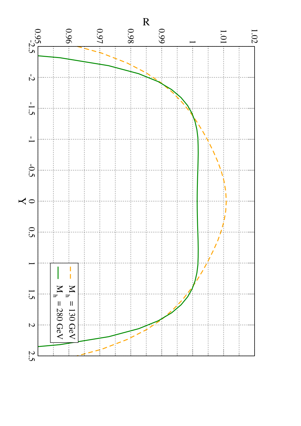
Refer to captionRefer to caption
Figure 5: The ratio of the rapidity distribution for Higgs production computed up to NLO using the matched expressions Eqs. (152-154) to the result in the heavy top limit of Ref. [25]. The ratio is rescaled by the corresponding ratio of total cross-sections. Results are shown for the LHC at 77 TeV (left) and 1414 TeV (right); the dashed yellow curves are for mh=130m_{h}=130 GeV and the solid green ones for mh=280m_{h}=280 GeV.

6 Conclusions and Outlook

In this paper we have accomplished for the first time small xx resummation of a differential cross-section (as opposed to a fully inclusive one). This has been done by extending to differential rapidity distributions the so-called high energy or kTk_{T} factorization, which expresses LLxx cross-sections in terms of standard partonic cross-sections, but computed with incoming off-shell gluons. The result has been made possible by exploiting the duality which relates LLxx and LLQ2Q^{2} evolution equations, to re-express high energy factorization in terms of standard collinear factorization, which in turns is straightforwardly extended to rapidity distributions.

Our final resummation prescription is quite close to the well-established one derived long ago for inclusive cross-sections [1]. Indeed, it is based on evaluating the LO rapidity distribution for the relevant process but with incoming off-shell gluons. As in the inclusive case, the leading high energy behavior is found by means of a pole approximation in Mellin space, whereby the Mellin variable which is conjugate to the gluon virtuality is identified with the LLxx anomalous dimension. However, one must now also take a Fourier transform with respect to rapidity, and the argument of LLxx anomalous dimensions undergoes an impact-parameter dependent shift in the complex plane of the variable which is Mellin conjugate to the scaling variable xx.

As first application, we have performed a resummation of the rapidity distribution for Higgs production in gluon-gluon fusion. We have computed the small xx limit of the rapidity distribution to NNLO, both in the heavy top mass approximation and for finite mtopm_{\rm top} (only the mtop→∞m_{\rm top}\to\infty NLO result being already available in closed form). We have shown the way these expressions are related to the results obtained by expanding to finite order the resummation formula and inverting the Fourier-Mellin transform, and we have seen that this involves nontrivial cancellations between terms which at the resummed level have different origins, thereby providing a nontrivial consistency check on the resummation procedure. As a first example of application we have constructed an approximate analytic expression for the NLO rapidity distribution with finite top mass, which appears to be in agreement with the numerical results of Ref. [27], but provides a prediction which is not affected by problems of numerical accuracy.

The potentially more interesting application of this formalism is to Drell-Yan rapidity distributions, which will be explored at very small xx at the LHC, specifically by the LHCb collaboration [18], and which may play an important role both in determining parton distributions and testing resummed QCD predictions at small xx. More in general, our result provide a first generalization of small xx factorization and resummation beyond the inclusive LLxx level. It will be interesting to see whether they can be generalized not only to less inclusive quantities, but also beyond the leading logarithmic approximation.

Acknowledgment We thank R. D. Ball for several discussions which are at the origin of this paper and for a critical reading of the manuscript. F.C. acknowledges many useful discussions with G. Diana, S.F. thanks V. del Duca for discussions during the early stage of this work, and S.M. thanks F. Petriello for fruitful correspondence on the fixed-order results. This work was supported in part by the European network HEPTOOLS under contract MRTN-CT-2006-035505 and by an Italian PRIN-2008 grant. The work of S.M. is supported by UK’s STFC.

Appendix

Appendix A The MS¯\overline{\textsc{MS}} subtraction procedure to all orders

Here we briefly sketch how to subtract collinear singularities arising from kernel iteration within the MS¯\overline{\textsc{MS}} scheme. Here we outline only the features which are relevant to understand how Eqs. (31), (42) are obtained. For a general treatment, including a discussion of ultraviolet and infrared singularities, as well as for a more detailed explanation, we refer the reader to the original papers [30, 21].

We start by writing a generic cross-section as the convolution product of a “bare” (i.e. unsubtracted) coefficient function M¯\bar{M} and a “bare” PDF Γ¯\bar{\Gamma}:

σ=M¯⊗Γ¯,\sigma=\bar{M}\otimes\bar{\Gamma}, (159)

where ⊗\otimes denotes the standard convolution product in xx space. We assume to work in d=4−2​ϵd=4-2\epsilon dimensions in order to regularize M¯\bar{M} and Γ¯\bar{\Gamma}. Following Sect. 2, we now write the coefficient function M¯\bar{M} as the product of a hard part HH and the iteration of a kernel KK:

M¯=H⊗x,kT(1+K+K⊗x,kTK+…)≡M⁡(1+K+K2+K3+…)=H​11−K,\bar{M}=H\otimes_{x,k_{T}}(1+K+K\otimes_{x,k_{T}}K+...)\equiv M(1+K+K^{2}+K^{3}+...)=H{{1}\over{1-K}}, (160)

where now the convolution ⊗x,kT\otimes_{x,k_{T}} stands both for normal convolution in xx space and for kTk_{T} integration in the transverse space. This convolution product will be understood in the following formal manipulations.

As a result of the kTk_{T} integrations, the coefficient function Eq. (160) contains multiple collinear poles of the form 1/ϵj1/\epsilon^{j} and thus it is meaningless in 4 dimensions. To perform the subtraction, we first introduce the “pole-part” projector PP which acting on a generic function FF selects just its 1/ϵk1/\epsilon^{k} poles, i.e.

P​F≡∑k>01ϵk​limϵ→0(ϵk​F).PF\equiv\sum_{k>0}{{1}\over{\epsilon^{k}}}\lim_{\epsilon\rightarrow 0}\left(\epsilon^{k}F\right). (161)

We now use this projector to factorize the kernel 1/(1−K)1/(1-K) in Eq. (160) into a finite part and a pure-pole part. To this purpose, we first consider the kernel (1−K)(1-K) and perform the following formal manipulations:

1−K=1−P​K−(1−P)​K=[1−P​K​(1−(1−P)​K)−1]​[1−(1−P)​K],1-K=1-PK-(1-P)K=\left[1-PK(1-(1-P)K)^{-1}\right]\left[1-(1-P)K\right], (162)

which leads to (note the reverse order):

11−K=[11−(1−P)​K]​[11−P​K​(1−(1−P)​K)−1].{{1}\over{1-K}}=\left[{{1}\over{1-(1-P)K}}\right]\left[{{1}\over{1-PK(1-(1-P)K)^{-1}}}\right]. (163)

This is the desired factorized expression: the term in the first square bracket is by construction free of collinear singularities, which have been moved to the second term. Using this factorized form, we can now rewrite the cross-section (159) as

σ=M¯​Γ¯={H⁡[11−(1−P)​K]}​{[11−P​K​(1−(1−P)​K)−1]​Γ¯}=M​Γ,\sigma=\bar{M}\bar{\Gamma}=\left\{H\left[{{1}\over{1-(1-P)K}}\right]\right\}\left\{\left[{{1}\over{1-PK(1-(1-P)K)^{-1}}}\right]\bar{\Gamma}\right\}=M\Gamma, (164)

with

M\displaystyle M ≡\displaystyle\equiv H⁡[11−(1−P)​K]\displaystyle H\left[{{1}\over{1-(1-P)K}}\right]
Γ\displaystyle\Gamma ≡\displaystyle\equiv [11−P​K​(1−(1−P)​K)−1]​Γ¯.\displaystyle\left[{{1}\over{1-PK(1-(1-P)K)^{-1}}}\right]\bar{\Gamma}. (165)

Now both MM and Γ\Gamma are finite, hence we can safely let ϵ=0\epsilon=0 and obtain a well-defined d=4d=4 result. Note that this subtraction scheme is uniquely defined once the action of PP is specified. The subtraction of the pure pole part (as in Eq. (161)) defines the MS scheme. In the MS¯\overline{\textsc{MS}} scheme one chooses to subtract also terms proportional to −γE+ln⁡4​π-\gamma_{E}+\ln 4\pi coming from angular integrations. At leading logarithmic accuracy the action of PP is defined as:

PMS¯​F=∑k>0(limϵ→0ϵk​F)×1ϵk​exp⁡[k​ϵ​(−γE+ln⁡4​π)].P_{\overline{\textsc{MS}}}~F=\sum_{k>0}\left(\lim_{\epsilon\rightarrow 0}\epsilon^{k}F\right)\times{{1}\over{\epsilon^{k}}}\exp\left[k\,\epsilon\left(-\gamma_{E}+\ln 4\pi\right)\right]. (166)

We now illustrate this subtraction procedure on the simple case of the t−t-channel iteration of Altarelli-Parisi gluons. In this case we have

K\displaystyle K =\displaystyle= (4​π)ϵΓ⁡(1−ϵ)​∫0Q2d​kT2(kT2)1+ϵ​αs​(μ2)ϵ​γ0​(N)=−1ϵ​(4​π)ϵΓ⁡(1−ϵ)​(αs​γ0​(N))​(μ2Q2)ϵ,\displaystyle{{(4\pi)^{\epsilon}}\over{\Gamma(1-\epsilon)}}\int_{0}^{Q^{2}}{{dk_{T}^{2}}\over{\left(k_{T}^{2}\right)^{1+\epsilon}}}\alpha_{s}\left(\mu^{2}\right)^{\epsilon}\gamma_{0}(N)=-{{1}\over{\epsilon}}{{(4\pi)^{\epsilon}}\over{\Gamma(1-\epsilon)}}\left(\alpha_{s}\gamma_{0}(N)\right)\left({{\mu^{2}}\over{Q^{2}}}\right)^{\epsilon},
K2\displaystyle K^{2} =\displaystyle= (4​π)ϵΓ⁡(1−ϵ)∫0Q2d​kT,22(kT,22)1+ϵ(αs(μ2)ϵγ0(N))(4​π)ϵΓ⁡(1−ϵ)×\displaystyle{{(4\pi)^{\epsilon}}\over{\Gamma(1-\epsilon)}}\int_{0}^{Q^{2}}{{dk_{T,2}^{2}}\over{\left(k_{T,2}^{2}\right)^{1+\epsilon}}}\left(\alpha_{s}\left(\mu^{2}\right)^{\epsilon}\gamma_{0}(N)\right){{(4\pi)^{\epsilon}}\over{\Gamma(1-\epsilon)}}\times
×\displaystyle\times ∫0kT,22d​kT,12(kT,12)1+ϵ​(αs​(μ2)ϵ​γ0​(N))=12​ϵ2​(4​π)2​ϵΓ2​(1−ϵ)​(αs​γ0​(N))2​(μ2Q2)2​ϵ\displaystyle\int_{0}^{k_{T,2}^{2}}{{dk_{T,1}^{2}}\over{\left(k_{T,1}^{2}\right)^{1+\epsilon}}}\left(\alpha_{s}\left(\mu^{2}\right)^{\epsilon}\gamma_{0}(N)\right)={{1}\over{2\epsilon^{2}}}{{(4\pi)^{2\epsilon}}\over{\Gamma^{2}(1-\epsilon)}}\left(\alpha_{s}\gamma_{0}(N)\right)^{2}\left({{\mu^{2}}\over{Q^{2}}}\right)^{2\epsilon}

and so on. Note that K2K^{2} contains both single and double poles:

K2αs2​γ02\displaystyle{{K^{2}}\over{\alpha_{s}^{2}\gamma_{0}^{2}}} =\displaystyle= 12​ϵ2+ln⁡(μ2Q2)+ln⁡(4​π)−γEϵ+(ln(μ2Q2)+ln(4π)−2γE)×\displaystyle{{1}\over{2\epsilon^{2}}}+{{\ln\left({{\mu^{2}}\over{Q^{2}}}\right)+\ln(4\pi)-\gamma_{E}}\over{\epsilon}}+\left(\ln\left({{\mu^{2}}\over{Q^{2}}}\right)+\ln(4\pi)-2\gamma_{E}\right)\times (168)
×(ln⁡(μ2Q2)+ln⁡(4​π))−π212+γE2+O⁡(ϵ).\displaystyle\quad\times\left(\ln\left({{\mu^{2}}\over{Q^{2}}}\right)+\ln(4\pi)\right)-{{\pi^{2}}\over{12}}+\gamma_{E}^{2}+O\left(\epsilon\right).

Careless subtraction of all poles and ln⁡(4​π)\ln(4\pi), γE\gamma_{E} terms would lead to the incorrect result

Ksub2=αs2​γ02​(N)​ln2​Q2μ2.K^{2}_{\text{sub}}=\alpha_{s}^{2}\gamma_{0}^{2}(N)\ln^{2}{{Q^{2}}\over{\mu^{2}}}. (169)

The correct MS¯\overline{\textsc{MS}} result is instead obtained following the procedure explained above: instead of subtracting poles from K2K^{2} we should consider (1−P)​[K​(1−P)​K](1-P)[K(1-P)K]. In this case we get

(1−P)​K\displaystyle(1-P)K =\displaystyle= (αs​γ0​(N))​(−1ϵ​(4​π)ϵΓ⁡(1−ϵ)​(μ2Q2)ϵ+Sϵϵ);\displaystyle\left(\alpha_{s}\gamma_{0}(N)\right)\left(-{{1}\over{\epsilon}}{{(4\pi)^{\epsilon}}\over{\Gamma(1-\epsilon)}}\left({{\mu^{2}}\over{Q^{2}}}\right)^{\epsilon}+{{S_{\epsilon}}\over{\epsilon}}\right);
K⁡(1−P)​K\displaystyle K(1-P)K =\displaystyle= (αs​γ0​(N))2​(12​ϵ2​(4​π)2​ϵΓ2​(1−ϵ)​(μ2Q2)2​ϵ+CLOSE\displaystyle\left(\alpha_{s}\gamma_{0}(N)\right)^{2}\left({{1}\over{2\epsilon^{2}}}{{(4\pi)^{2\epsilon}}\over{\Gamma^{2}(1-\epsilon)}}\left({{\mu^{2}}\over{Q^{2}}}\right)^{2\epsilon}+\right. (170)
OPEN−1ϵ2​(4​π)ϵΓ⁡(1−ϵ)​(μ2Q2)ϵ​Sϵ);\displaystyle-\left.{{1}\over{\epsilon^{2}}}{{(4\pi)^{\epsilon}}\over{\Gamma(1-\epsilon)}}\left({{\mu^{2}}\over{Q^{2}}}\right)^{\epsilon}S_{\epsilon}\right);
(1−P)​[K​(1−P)​K]\displaystyle(1-P)\left[K(1-P)K\right] =\displaystyle= (αs​γ0​(N))2​(12​ϵ2​(4​π)2​ϵΓ2​(1−ϵ)​(μ2Q2)2​ϵ+CLOSE\displaystyle\left(\alpha_{s}\gamma_{0}(N)\right)^{2}\left({{1}\over{2\epsilon^{2}}}{{(4\pi)^{2\epsilon}}\over{\Gamma^{2}(1-\epsilon)}}\left({{\mu^{2}}\over{Q^{2}}}\right)^{2\epsilon}+\right. (171)
OPEN−1ϵ2​(4​π)ϵΓ⁡(1−ϵ)​(μ2Q2)ϵ​Sϵ+12​ϵ2​Sϵ2)=\displaystyle\left.-{{1}\over{\epsilon^{2}}}{{(4\pi)^{\epsilon}}\over{\Gamma(1-\epsilon)}}\left({{\mu^{2}}\over{Q^{2}}}\right)^{\epsilon}S_{\epsilon}+{{1}\over{2\epsilon^{2}}}S_{\epsilon}^{2}\right)=
=\displaystyle= (αs​γ0​(N))2​12​ϵ2​((4​π)ϵΓ⁡(1−ϵ)​(μ2Q2)ϵ−Sϵ)2;\displaystyle\left(\alpha_{s}\gamma_{0}(N)\right)^{2}{{1}\over{2\epsilon^{2}}}\left({{(4\pi)^{\epsilon}}\over{\Gamma(1-\epsilon)}}\left({{\mu^{2}}\over{Q^{2}}}\right)^{\epsilon}-S_{\epsilon}\right)^{2};

with Sϵ≡exp⁡[ϵ⁡(ln⁡(4​π)−γE)]S_{\epsilon}\equiv\exp\left[\epsilon\left(\ln(4\pi)-\gamma_{E}\right)\right]. Note that this time

(1−P)​[K⁡(1−P)​K]=12​(αs​γ0)2​ln2​Q2μ2+O⁡(ϵ),(1-P)\left[K(1-P)K\right]={{1}\over{2}}\left(\alpha_{s}\gamma_{0}\right)^{2}\ln^{2}{{Q^{2}}\over{\mu^{2}}}+O(\epsilon), (172)

which is the correct MS¯\overline{\textsc{MS}} result.

This subtraction procedure can be easily iterated. In particular, with nn kernels the result is

(1−P)​K​…​(1−P)​K\displaystyle(1-P)K...(1-P)K =\displaystyle= (αs​γ0)n​(−1)nn!​1ϵn​((4​π)ϵΓ⁡(1−ϵ)​(μ2Q2)ϵ−Sϵ)n=\displaystyle\left(\alpha_{s}\gamma_{0}\right)^{n}{{(-1)^{n}}\over{n!}}{{1}\over{\epsilon^{n}}}\left({{(4\pi)^{\epsilon}}\over{\Gamma(1-\epsilon)}}\left({{\mu^{2}}\over{Q^{2}}}\right)^{\epsilon}-S_{\epsilon}\right)^{n}= (173)
=\displaystyle= (αs​γ0)n​1n!​lnn​Q2μ2+O⁡(ϵ).\displaystyle\left(\alpha_{s}\gamma_{0}\right)^{n}{{1}\over{n!}}\ln^{n}{{Q^{2}}\over{\mu^{2}}}+O(\epsilon).

Note that before performing the last (1−P)(1-P) subtraction, the nn-kernel result contains only a single 1/ϵn1/\epsilon^{n} pole.

A particularly important feature of this subtraction method is its iterative nature. This is especially well suited for the purpose of this paper, because we can perform all the universal kernel subtractions once for all, and consider separately the single collinear divergence coming from attaching the universal ladder to the process-dependent hard coefficient function, see Eqs. (31), (42). Also, the MS¯\overline{\textsc{MS}} subtraction factor SϵS_{\epsilon} exactly cancels all terms coming from (4​π)ϵ/Γ⁡(1−ϵ)(4\pi)^{\epsilon}/\Gamma(1-\epsilon): the full MS¯\overline{\textsc{MS}} result can be obtained by just neglecting all (4​π)ϵ/Γ⁡(1−ϵ)(4\pi)^{\epsilon}/\Gamma(1-\epsilon) terms and using Sϵ=1S_{\epsilon}=1. This simplification only relies on the fact that each emission is accompanied exactly by a (4​π)ϵ/Γ⁡(1−ϵ)(4\pi)^{\epsilon}/\Gamma(1-\epsilon) term, which happens if there are no angular correlations. Since in all our derivations angular correlations are subleading, in the main paper we have used this simplified version of the subtraction procedure.

Appendix B Resummation of rapidity distributions in MS¯\overline{\textsc{MS}}

In this appendix we provide an explicit derivation of the resummation of the rapidity distribution in the MS¯\overline{\textsc{MS}} scheme. Because rapidity is determined by the longitudinal momentum components, while collinear singularities appear in transverse momentum integrations, the main features of the MS¯\overline{\textsc{MS}} derivation are the same of the derivation in Sec. 3.

For simplicity we consider emissions from just one leg. Extension to the full case is straightforward. We start by writing the n−n-kernel fully differential cross-section in d=4−2​ϵd=4-2\epsilon dimensions, see Eq. (2.4) 66 6 Here again we omit all (4​π)ϵ/Γ⁡(1−ϵ)(4\pi)^{\epsilon}/\Gamma(1-\epsilon) terms in view of the MS¯\overline{\textsc{MS}} subtraction, as discussed in Appendix A.:

dσ¯n(x,μ2Q2,αs,zi,ξi;ϵ,)=\displaystyle{d}\bar{\sigma}^{n}\left(x,{{\mu^{2}}\over{Q^{2}}},\alpha_{s},z_{i},\xi_{i};\epsilon,\right)=
P(zn,(μ2Q2)ϵ,αs;ϵ)d​znznd​ξnξn1+ϵ×C(x,zi,ξi,αs;ϵ)×\displaystyle P\left(z_{n},\left({{\mu^{2}}\over{Q^{2}}}\right)^{\epsilon},\alpha_{s};\epsilon\right){{dz_{n}}\over{z_{n}}}{{d\xi_{n}}\over{\xi_{n}^{1+\epsilon}}}\times C\left(x,z_{i},\xi_{i},\alpha_{s};\epsilon\right)\times
×P⁡(zn−1,(μ2Q2)ϵ,αs,ϵ)​d​zn−1zn−1​d​ξn−1ξn−11+ϵ×…×P⁡(z1,(μ2Q2)ϵ,αs,ϵ)​d​z1z1​d​ξ1ξ11+ϵ,\displaystyle\times P\left(z_{n-1},\left({{\mu^{2}}\over{Q^{2}}}\right)^{\epsilon},\alpha_{s};\epsilon\right){{dz_{n-1}}\over{z_{n-1}}}{{d\xi_{n-1}}\over{\xi_{n-1}^{1+\epsilon}}}\times...\times P\left(z_{1},\left({{\mu^{2}}\over{Q^{2}}}\right)^{\epsilon},\alpha_{s};\epsilon\right){{dz_{1}}\over{z_{1}}}{{d\xi_{1}}\over{\xi_{1}^{1+\epsilon}}},

where as in Eq. (73) the splitting function PP is the inverse Mellin transform of the anomalous dimension γ\gamma in Eq. (2.4). Note that in Eq. (B) we have written CC as the most generic (2PI) function of all the relevant variables. Quasi-collinear kinematics determines the dependence of CC on its arguments. Because rapidity distributions do not factorize in N−N-Mellin space, for the time being we write everything in x−x-space.

The d−d-dimensional rapidity distribution is immediately obtained from the fully differential cross-section Eq. (B):

d​σ¯nd​y​(x,μ2Q2,y,αs,ϵ)=\displaystyle{{{d}\bar{\sigma}^{n}}\over{{d}y}}\left(x,{{\mu^{2}}\over{Q^{2}}},y,\alpha_{s};\epsilon\right)=
=∫x1d​znznP(zn,(μ2Q2)ϵ,αs;ϵ)×…×∫xz2​…​zn1d​z1z1P(z1,(μ2Q2)ϵ,αs;ϵ)×\displaystyle\quad=\int_{x}^{1}{{dz_{n}}\over{z_{n}}}P\left(z_{n},\left({{\mu^{2}}\over{Q^{2}}}\right)^{\epsilon},\alpha_{s};\epsilon\right)\times...\times\int_{{{x}\over{z_{2}...z_{n}}}}^{1}{{dz_{1}}\over{z_{1}}}P\left(z_{1},\left({{\mu^{2}}\over{Q^{2}}}\right)^{\epsilon},\alpha_{s};\epsilon\right)\times
×∫0∞d​ξnξn1+ϵ​Cy​(x,zi,ξi,y,αs,ϵ)​∫0ξnd​ξn−1ξn−11+ϵ×…×∫0ξ2d​ξ1ξ11+ϵ,\displaystyle\qquad\times\int_{0}^{\infty}{{d\xi_{n}}\over{\xi_{n}^{1+\epsilon}}}C_{y}\left(x,z_{i},\xi_{i},y,\alpha_{s};\epsilon\right)\int_{0}^{\xi_{n}}{{d\xi_{n-1}}\over{\xi_{n-1}^{1+\epsilon}}}\times...\times\int_{0}^{\xi_{2}}{{d\xi_{1}}\over{\xi_{1}^{1+\epsilon}}},

where the rapidity-dependent coefficient function is defined as

Cy(x,zi,ξi,y,αs;ϵ)≡Q22​s​z1​…​zn∫02​πd​θ2​π∫dΠℱ|ℳ⁡(𝒱⁡(n)+g∗​(pL)→ℱ)|2¯×\displaystyle C_{y}\left(x,z_{i},\xi_{i},y,\alpha_{s};\epsilon\right)\equiv{{Q^{2}}\over{2sz_{1}...z_{n}}}\int_{0}^{2\pi}{{d\theta}\over{2\pi}}\int d\Pi_{\mathcal{F}}\overline{\left|\mathcal{M}\left(\mathcal{V}(n)+g^{*}(p_{L})\rightarrow\mathcal{F}\right)\right|^{2}}\times
×δ4​(PI−Pf)×δ⁡(y−12​ln⁡E𝒮+p𝒮​zE𝒮−p𝒮​z),\displaystyle\quad\times\delta_{4}(P_{I}-P_{f})\times\delta\left(y-{{1}\over{2}}\ln{{E_{\mathcal{S}}+p_{\mathcal{S}z}}\over{E_{\mathcal{S}}-p_{\mathcal{S}z}}}\right), (176)

in terms of the spin and color averaged squared amplitude |ℳ|2¯\overline{\left|\mathcal{M}\right|^{2}} for the off-shell process 𝒱⁡(n)+g∗​(pL)→ℱ\mathcal{V}(n)+g^{*}(p_{L})\rightarrow\mathcal{F} (see Fig. 2), and the polarization sum for the off-shell gluon is performed through the projector 𝒫\mathcal{P} Eq. (12). We now use the fact that we are in quasi-collinear kinematics (i.e. ξi≪ξi+1\xi_{i}\ll\xi_{i+1}) and in the small xx regime Eq. (8). This implies first, that CyC_{y} is sensitive only to the largest transverse momenta ξn\xi_{n} and second, that up to terms which vanish when kT2≪sk_{T}^{2}\ll s the effect of the ladder insertion to CyC_{y} is just a longitudinal boost. We have thus

Cy​(x,zi,ξi,y,αs,ϵ)=\displaystyle C_{y}(x,z_{i},\xi_{i},y,\alpha_{s};\epsilon)=
=Cy​(xz1​…​zn,ξn,y−12​ln⁡z1−…−12​ln⁡zn,αs,ϵ)+O⁡(kT2s).\displaystyle\quad=C_{y}\left({{x}\over{z_{1}...z_{n}}},\xi_{n},y-{{1}\over{2}}\ln z_{1}-...-{{1}\over{2}}\ln z_{n},\alpha_{s};\epsilon\right)+O\left({{k_{T}^{2}}\over{s}}\right). (177)

Since upon integration O⁡(kT2/s)O(k_{T}^{2}/s) terms give rise to contributions suppressed by powers of xx, we can safely discard them.

Thanks to quasi-collinear kinematics we can thus write Eq. (B) as

d​σ¯nd​y​(x,μ2Q2,y,αs,ϵ)=\displaystyle{{{d}\bar{\sigma}^{n}}\over{{d}y}}\left(x,{{\mu^{2}}\over{Q^{2}}},y,\alpha_{s};\epsilon\right)=
=∫x1d​znznP(zn,(μ2Q2)ϵ,αs;ϵ)×…×∫xz2​…​zn1d​z1z1P(z1,(μ2Q2)ϵ,αs;ϵ)×\displaystyle=\int_{x}^{1}{{dz_{n}}\over{z_{n}}}P\left(z_{n},\left({{\mu^{2}}\over{Q^{2}}}\right)^{\epsilon},\alpha_{s};\epsilon\right)\times...\times\int_{{{x}\over{z_{2}...z_{n}}}}^{1}{{dz_{1}}\over{z_{1}}}P\left(z_{1},\left({{\mu^{2}}\over{Q^{2}}}\right)^{\epsilon},\alpha_{s};\epsilon\right)\times
×∫0∞d​ξnξn1+ϵCy(xz1​…​zn,ξn,y−12lnz1−…−12lnzn,αs;ϵ)×\displaystyle\times\int_{0}^{\infty}{{d\xi_{n}}\over{\xi_{n}^{1+\epsilon}}}C_{y}\left({{x}\over{z_{1}...z_{n}}},\xi_{n},y-{{1}\over{2}}\ln z_{1}-...-{{1}\over{2}}\ln z_{n},\alpha_{s};\epsilon\right)\times
×∫0ξnd​ξn−1ξn−11+ϵ×…×∫0ξ2d​ξ1ξ11+ϵ+O⁡(x).\displaystyle\times\int_{0}^{\xi_{n}}{{d\xi_{n-1}}\over{\xi_{n-1}^{1+\epsilon}}}\times...\times\int_{0}^{\xi_{2}}{{d\xi_{1}}\over{\xi_{1}^{1+\epsilon}}}+O(x). (178)

From now on we will systematically omit all O⁡(x)O(x) terms.

Convolution products in Eq. (178) turn into ordinary ones by Fourier-Mellin transformation:

d​σ¯nd​y(N,μ2Q2,b,αs;ϵ)=[γ(N−i​b2,(μ2Q2)ϵ,αs;ϵ)]×\displaystyle{{{d}\bar{\sigma}^{n}}\over{{d}y}}\left(N,{{\mu^{2}}\over{Q^{2}}},b,\alpha_{s};\epsilon\right)=\left[\gamma\left(N-{{ib}\over{2}},\left({{\mu^{2}}\over{Q^{2}}}\right)^{\epsilon},\alpha_{s};\epsilon\right)\right]\times
×∫0∞d​ξnξn1+ϵCy(N,ξn,b,αs;ϵ)×∫0ξn[γ(N−i​b2,(μ2Q2)ϵ,αs;ϵ)]d​ξn−1ξn−11+ϵ×\displaystyle\quad\times\int_{0}^{\infty}{{d\xi_{n}}\over{\xi_{n}^{1+\epsilon}}}C_{y}\left(N,\xi_{n},b,\alpha_{s};\epsilon\right)\times\int_{0}^{\xi_{n}}\left[\gamma\left(N-{{ib}\over{2}},\left({{\mu^{2}}\over{Q^{2}}}\right)^{\epsilon},\alpha_{s};\epsilon\right)\right]{{d\xi_{n-1}}\over{\xi_{n-1}^{1+\epsilon}}}\times
×…×∫0ξ2[γ⁡(N−i​b2,(μ2Q2)ϵ,αs,ϵ)]​d​ξ1ξ11+ϵ.\displaystyle\quad\times...\times\int_{0}^{\xi_{2}}\left[\gamma\left(N-{{ib}\over{2}},\left({{\mu^{2}}\over{Q^{2}}}\right)^{\epsilon},\alpha_{s};\epsilon\right)\right]{{d\xi_{1}}\over{\xi_{1}^{1+\epsilon}}}. (179)

This expression is identical to Eq. (2.4), but with the anomalous dimension γ\gamma is evaluated at N−i​b/2N-ib/2. This does not interfere with collinear singularities, hence the MS¯\overline{\textsc{MS}} subtraction is performed as in the inclusive case, with the result (see Eq. (44))

d​σd​y=∑n=1∞d​σ¯nd​y=γ(N−i​b2,(μ2Q2)ϵ,αs;ϵ)∫0∞d​ξξ1+ϵCy(N,ξ,b,αs;ϵ)×\displaystyle{{{d}\sigma}\over{{d}y}}=\sum_{n=1}^{\infty}{{{d}\bar{\sigma}^{n}}\over{{d}y}}=\gamma\left(N-{{ib}\over{2}},\left({{\mu^{2}}\over{Q^{2}}}\right)^{\epsilon},\alpha_{s};\epsilon\right)\int_{0}^{\infty}{{d\xi}\over{\xi^{1+\epsilon}}}C_{y}\left(N,\xi,b,\alpha_{s};\epsilon\right)\times
×exp⁡[1ϵ​∑kγ~k​(N−i​b2,αs,0)k​(1−(μ2Q2​ξ)k​ϵ​γ~k​(N−i​b/2,αs,ϵ)γ~k​(N−i​b/2,αs,0))],\displaystyle\times\exp\left[{{1}\over{\epsilon}}\sum_{k}{{\tilde{\gamma}_{k}\left(N-{{ib}\over{2}},\alpha_{s};0\right)}\over{k}}\left(1-\left({{\mu^{2}}\over{Q^{2}\xi}}\right)^{k\epsilon}{{\tilde{\gamma}_{k}(N-ib/2,\alpha_{s};\epsilon)}\over{\tilde{\gamma}_{k}(N-ib/2,\alpha_{s};0)}}\right)\right],

where γ~k\tilde{\gamma}_{k} was defined in Eq. (45). As in the inclusive case, Eq. (B) has a finite ϵ→0\epsilon\to 0 limit:

limϵ→0\displaystyle\lim_{\epsilon\rightarrow 0} 1ξ1+ϵ​exp⁡[1ϵ​∑iα¯sii​γi​(N−i​b2,0)​(1−(μ2Q2​ξ)i​ϵ​γi​(N−i​b/2,ϵ)γi​(N−i​b/2,0))]=\displaystyle{{1}\over{\xi^{1+\epsilon}}}\exp\left[{{1}\over{\epsilon}}\sum_{i}{{\bar{\alpha}_{s}^{i}}\over{i}}\gamma_{i}\left(N-{{ib}\over{2}},0\right)\left(1-\left({{\mu^{2}}\over{Q^{2}\xi}}\right)^{i\epsilon}{{\gamma_{i}(N-ib/2,\epsilon)}\over{\gamma_{i}(N-ib/2,0)}}\right)\right]= (181)
=\displaystyle= ξγ⁡(N−i​b2,αs)−1exp[γ(N−i​b2,αs)lnQ2μ2]e−∑iαsi​γ˙i​(N−i​b/2)i=\displaystyle\xi^{\gamma\left(N-{{ib}\over{2}},\alpha_{s}\right)-1}\exp\left[\gamma\left(N-{{ib}\over{2}},\alpha_{s}\right)\ln{{Q^{2}}\over{\mu^{2}}}\right]e^{-\sum_{i}{{\alpha_{s}^{i}\dot{\gamma}_{i}(N-ib/2)}\over{i}}}=
=\displaystyle= ξγ⁡(N−i​b2,αs)−1​exp⁡[γ⁡(N−i​b2,αs)​ln⁡Q2μ2]​ℛ​(N−i​b2,αs).\displaystyle\xi^{\gamma\left(N-{{ib}\over{2}},\alpha_{s}\right)-1}\exp\left[\gamma\left(N-{{ib}\over{2}},\alpha_{s}\right)\ln{{Q^{2}}\over{\mu^{2}}}\right]\mathcal{R}\left(N-{{ib}\over{2}},\alpha_{s}\right).

Using Eq. (181) the resummed result immediately follows (with μ2=Q2\mu^{2}=Q^{2}, thus omitting the explicit dependence on μ2/Q2\mu^{2}/Q^{2}):

d​σd​y(N,αs(Q2),b)=γ(N−i​b2,αs(Q2))×\displaystyle{{{d}\sigma}\over{{d}y}}(N,\alpha_{s}(Q^{2}),b)=\gamma\left(N-{{ib}\over{2}},\alpha_{s}(Q^{2})\right)\times
×∫0∞d​ξ​ξγ⁡(N−i​b/2,αs​(Q2))−1​C​(N,ξ,αs​(Q2),b)​ℛ​(N−i​b2,αs​(Q2)),\displaystyle\times\int_{0}^{\infty}d\xi\xi^{\gamma\left(N-ib/2,\alpha_{s}(Q^{2})\right)-1}C\left(N,\xi,\alpha_{s}(Q^{2}),b\right)\mathcal{R}\left(N-{{ib}\over{2}},\alpha_{s}(Q^{2})\right), (182)

which is the same of Eq.(47) but this time with a shifted ℛ\mathcal{R} factor. Note that at LLxx we also have

γ⁡(N−i​b2,αs)=γ⁡(αsN−i​b/2);ℛ⁡(N−i​b2,αs)=ℛ⁡(αsN−i​b/2).\gamma\left(N-{{ib}\over{2}},\alpha_{s}\right)=\gamma\left({{\alpha_{s}}\over{N-ib/2}}\right);\qquad\mathcal{R}\left(N-{{ib}\over{2}},\alpha_{s}\right)=\mathcal{R}\left({{\alpha_{s}}\over{N-ib/2}}\right). (183)

We finally show how to deal with a scheme change in rapidity distribution, thereby in particular explaining the shift in the argument of ℛ\mathcal{R} in Eq. (182). To this purpose, assume a scheme change from MS¯\overline{\textsc{MS}} to some “small xx” scheme is performed by dividing the parton distribution by a LLxx function 𝒩{\mathcal{N}}:

Msmall​x≡MMS¯​𝒩;Γsmall​x≡1𝒩​ΓMS¯.M_{\rm{small}~x}\equiv M_{\overline{\textsc{MS}}}\mathcal{N};\qquad\Gamma_{\rm{small}~x}\equiv{{1}\over{\mathcal{N}}}\Gamma_{\overline{\textsc{MS}}}. (184)

Using the MS¯\overline{\textsc{MS}} kernel expansion Eq. (165) we can rewrite Msmall​xM_{\rm{small}~x} as

Msmall​x=H​11−(1−P)​K​𝒩=H⁡[1+(1−P)​K+(1−P)​[K⁡(1−P)​K]+…]​𝒩.M_{\rm{small}~x}=H{{1}\over{1-(1-P)K}}\mathcal{N}=H\left[1+(1-P)K+(1-P)\left[K(1-P)K\right]+...\right]\mathcal{N}. (185)

where (see Appendix A) all products must be understood as convolution in xx and kTk_{T} spaces. It follows that the effect of the scheme change is the same as that of a kernel insertion on the first (outer) rung of the ladder:

d​σ¯1d​y(x,μ2Q2,y,αs;ϵ)=∫x1d​zz𝒩(z,αs;ϵ)×\displaystyle{{{d}\bar{\sigma}^{1}}\over{{d}y}}\left(x,{{\mu^{2}}\over{Q^{2}}},y,\alpha_{s};\epsilon\right)=\int_{x}^{1}{{dz}\over{z}}\mathcal{N}\left(z,\alpha_{s};\epsilon\right)\times
×∫x/zd​z1z1​P​(z1,αs,(μ2Q2)ϵ,ϵ)​∫0∞d​ξξ1+ϵ​C​(xz​z1,ξ,y−12​ln⁡z−12​ln⁡z1,αs,ϵ).\displaystyle\quad\times\int_{x/z}{{dz_{1}}\over{z_{1}}}P\left(z_{1},\alpha_{s},\left({{\mu^{2}}\over{Q^{2}}}\right)^{\epsilon};\epsilon\right)\int_{0}^{\infty}{{d\xi}\over{\xi^{1+\epsilon}}}C\left({{x}\over{zz_{1}}},\xi,y-{{1}\over{2}}\ln z-{{1}\over{2}}\ln z_{1},\alpha_{s};\epsilon\right).

In Fourier-Mellin space the convolutions in Eq. (B) turn into ordinary products

d​σ¯1d​y(N,μ2Q2,b,αs;ϵ)=𝒩(N−i​b2,αs;ϵ)×\displaystyle{{{d}\bar{\sigma}^{1}}\over{{d}y}}\left(N,{{\mu^{2}}\over{Q^{2}}},b,\alpha_{s};\epsilon\right)=\mathcal{N}\left(N-{{ib}\over{2}},\alpha_{s};\epsilon\right)\times
×γ⁡(N−i​b2,αs,(μ2Q2)ϵ,ϵ)​∫0∞d​ξξ1+ϵ​Cy​(N−i​b2,b,αs,ϵ),\displaystyle\quad\times\gamma\left(N-{{ib}\over{2}},\alpha_{s},\left({{\mu^{2}}\over{Q^{2}}}\right)^{\epsilon};\epsilon\right)\int_{0}^{\infty}{{d\xi}\over{\xi^{1+\epsilon}}}C_{y}\left(N-{{ib}\over{2}},b,\alpha_{s};\epsilon\right), (187)

so the argument of 𝒩\mathcal{N} ends up being also shifted when used for computing rapidity distributions. Clearly this holds also if we consider the full ladder and not only a single kernel insertion.

Collecting the results of this section, we can write the full MS¯\overline{\textsc{MS}} rapidity distribution resummation formula as

d​σd​y(N,μ2Q2,b,αs(μ2))=[γ(αs​(μ2)N−i​b2)exp[γ(αs​(μ2)N−i​b2)lnQ2μ2]×\displaystyle{{{d}\sigma}\over{{d}y}}\left(N,{{\mu^{2}}\over{Q^{2}}},b,\alpha_{s}(\mu^{2})\right)=\left[\gamma\left({{\alpha_{s}(\mu^{2})}\over{N-{{ib}\over{2}}}}\right)\exp\left[\gamma\left({{\alpha_{s}(\mu^{2})}\over{N-{{ib}\over{2}}}}\right)\ln{{Q^{2}}\over{\mu^{2}}}\right]\times\right.
×∫0∞dξξγ⁡(αs​(μ2)N−i​b/2)−1C(N,ξ,b,αs(μ2))]R(αs​(μ2)N−i​b2).\displaystyle\times\left.\int_{0}^{\infty}d\xi\xi^{\gamma\left({{\alpha_{s}(\mu^{2})}\over{N-ib/2}}\right)-1}C\left(N,\xi,b,\alpha_{s}(\mu^{2})\right)\right]R\left({{\alpha_{s}(\mu^{2})}\over{N-{{ib}\over{2}}}}\right). (188)

The extension of Eq. (188) to emissions from both legs along the lines of Sec. 3 is straightforward

d​σd​y(N,μ2Q2,b,αs(μ2))=γ(αs​(μ2)N−i​b2)exp[γ(αs​(μ2)N−i​b2)lnQ2μ2]×\displaystyle{{{d}\sigma}\over{{d}y}}\left(N,{{\mu^{2}}\over{Q^{2}}},b,\alpha_{s}(\mu^{2})\right)=\gamma\left({{\alpha_{s}(\mu^{2})}\over{N-{{ib}\over{2}}}}\right)\exp\left[\gamma\left({{\alpha_{s}(\mu^{2})}\over{N-{{ib}\over{2}}}}\right)\ln{{Q^{2}}\over{\mu^{2}}}\right]\times
×γ(αs​(μ2)N+i​b2)exp[γ(αs​(μ2)N+i​b2)lnQ2μ2]×R(αs​(μ2)N−i​b2)R(αs​(μ2)N+i​b2)×\displaystyle\quad\times\gamma\left({{\alpha_{s}(\mu^{2})}\over{N+{{ib}\over{2}}}}\right)\exp\left[\gamma\left({{\alpha_{s}(\mu^{2})}\over{N+{{ib}\over{2}}}}\right)\ln{{Q^{2}}\over{\mu^{2}}}\right]\times R\left({{\alpha_{s}(\mu^{2})}\over{N-{{ib}\over{2}}}}\right)R\left({{\alpha_{s}(\mu^{2})}\over{N+{{ib}\over{2}}}}\right)\times
×∫0∞d​ξ​ξγ⁡(αs​(μ2)N−i​b/2)−1​∫0∞d​ξ¯​ξ¯γ⁡(αs​(μ2)N+i​b/2)−1​C​(N,ξ,ξ¯,b,αs​(μ2)).\displaystyle\quad\times\int_{0}^{\infty}d\xi\xi^{\gamma\left({{\alpha_{s}(\mu^{2})}\over{N-ib/2}}\right)-1}\int_{0}^{\infty}d\bar{\xi}\bar{\xi}^{\gamma\left({{\alpha_{s}(\mu^{2})}\over{N+ib/2}}\right)-1}C\left(N,\xi,\bar{\xi},b,\alpha_{s}(\mu^{2})\right). (189)

References

  • [1] S. Catani, M. Ciafaloni and F. Hautmann, Nucl. Phys. B 366 (1991) 135.
  • [2] S. Catani and F. Hautmann, Nucl. Phys. B 427 (1994) 475 [arXiv:hep-ph/9405388].
  • [3] R. D. Ball and R. K. Ellis, JHEP 0105 (2001) 053 [arXiv:hep-ph/0101199].
  • [4] F. Hautmann, Phys. Lett. B 535, 159 (2002) [arXiv:hep-ph/0203140].
  • [5] S. Marzani, R. D. Ball, V. Del Duca, S. Forte and A. Vicini, Nucl. Phys. B 800, 127 (2008) [arXiv:0801.2544 [hep-ph]].
  • [6] S. Marzani, R. D. Ball, V. Del Duca, S. Forte and A. Vicini, Nucl. Phys. Proc. Suppl. 186 (2009) 98 [arXiv:0809.4934 [hep-ph]].
  • [7] S. Marzani and R. D. Ball, Nucl. Phys. B 814, 246 (2009) [arXiv:0812.3602 [hep-ph]].
  • [8] G. Diana, Nucl. Phys. B 824, 154 (2010) [arXiv:0906.4159 [hep-ph]].
  • [9] R. V. Harlander, H. Mantler, S. Marzani and K. J. Ozeren, arXiv:0912.2104 [hep-ph].
  • [10] R. V. Harlander and K. J. Ozeren, JHEP 0911 (2009) 088 [arXiv:0909.3420 [hep-ph]].
  • [11] A. Pak, M. Rogal and M. Steinhauser, JHEP 1002 (2010) 025 [arXiv:0911.4662 [hep-ph]].
  • [12] L. N. Lipatov, Sov. J. Nucl. Phys. 23 (1976) 338 [Yad. Fiz. 23 (1976) 642]. E. A. Kuraev, L. N. Lipatov and V. S. Fadin, Sov. Phys. JETP 45, 199 (1977) [Zh. Eksp. Teor. Fiz. 72, 377 (1977)]. I. I. Balitsky and L. N. Lipatov, Sov. J. Nucl. Phys. 28, 822 (1978) [Yad. Fiz. 28, 1597 (1978)].
  • [13] V. S. Fadin and L. N. Lipatov, Phys. Lett. B 429 (1998) 127 [arXiv:hep-ph/9802290]. G. Camici and M. Ciafaloni, Phys. Lett. B 412 (1997) 396 [Erratum-ibid. B 417 (1998) 390] [arXiv:hep-ph/9707390].
  • [14] See M. Ciafaloni, D. Colferai, G. P. Salam and A. M. Stasto, Phys. Rev. D 68 (2003) 114003 [arXiv:hep-ph/0307188] and ref. therein.
  • [15] See G. Altarelli, R. D. Ball and S. Forte, Nucl. Phys. B 742 (2006) 1 [arXiv:hep-ph/0512237] and ref. therein.
  • [16] R. D. Ball, Nucl. Phys. B 796 (2008) 137 [arXiv:0708.1277 [hep-ph]].
  • [17] G. Altarelli, R. D. Ball and S. Forte, Nucl. Phys. B 799 (2008) 199 [arXiv:0802.0032 [hep-ph]].
  • [18] R. McNulty, In *Perugia 2008, Multiple Partonic Interactions at the LHC (MPI08)* 155-163
  • [19] S. Catani, M. Ciafaloni and F. Hautmann, Phys. Lett. B 307 (1993) 147.
  • [20] G. Altarelli, R. D. Ball and S. Forte, Nucl. Phys. B 575, 313 (2000).
  • [21] G. Curci, W. Furmanski and R. Petronzio, Nucl. Phys. B 175 (1980) 27.
  • [22] R. D. Ball and S. Forte, Phys. Lett. B 359 (1995) 362 [arXiv:hep-ph/9507321].
  • [23] M. Ciafaloni, Phys. Lett. B 356 (1995) 74 [arXiv:hep-ph/9507307].
  • [24] G. Altarelli, R. D. Ball and S. Forte, Nucl. Phys. B 599 (2001) 383 [arXiv:hep-ph/0011270].
  • [25] C. Anastasiou, L. J. Dixon and K. Melnikov, Nucl. Phys. Proc. Suppl. 116 (2003) 193 [arXiv:hep-ph/0211141].
  • [26] C. Anastasiou, K. Melnikov and F. Petriello, Nucl. Phys. B 724 (2005) 197 [arXiv:hep-ph/0501130].
  • [27] C. Anastasiou, S. Bucherer and Z. Kunszt, JHEP 0910 (2009) 068 [arXiv:0907.2362 [hep-ph]].
  • [28] T. Jaroszewicz, Phys. Lett. B 116, 291 (1982);
  • [29] M. Ciafaloni, Nucl. Phys. B 296 (1988) 49.
  • [30] R. K. Ellis, H. Georgi, M. Machacek, H. D. Politzer and G. G. Ross, Nucl. Phys. B 152 (1979) 285.
  • [31] M. Ciafaloni and D. Colferai, JHEP 0509 (2005) 069 [arXiv:hep-ph/0507106].
  • [32] S. Marzani, R. D. Ball, P. Falgari and S. Forte, Nucl. Phys. B 783 (2007) 143 [arXiv:0704.2404 [hep-ph]].
  • [33] M. Kramer, E. Laenen and M. Spira, Nucl. Phys. B 511 (1998) 523 [arXiv:hep-ph/9611272].
  • [34] C. Anastasiou, S. Bucherer and Z. Kunszt, JHEP 0910 (2009) 068 [arXiv:0907.2362 [hep-ph]].
  • [35] R. Kirschner and M. Segond, Eur. Phys. J. C 68 (2010) 425 [arXiv:0910.5443 [hep-ph]].
  • [36] R. D. Ball, L. Del Debbio, S. Forte, A. Guffanti, J. I. Latorre, J. Rojo and M. Ubiali, Nucl. Phys. B 838 (2010) 136 [arXiv:1002.4407 [hep-ph]].