An approximate dual subgradient algorithm for multi-agent non-convex optimization
Abstract
We consider a multi-agent optimization problem where agents subject to local, intermittent interactions aim to minimize a sum of local objective functions subject to a global inequality constraint and a global state constraint set. In contrast to previous work, we do not require that the objective, constraint functions, and state constraint sets to be convex. In order to deal with time-varying network topologies satisfying a standard connectivity assumption, we resort to consensus algorithm techniques and the Lagrangian duality method. We slightly relax the requirement of exact consensus, and propose a distributed approximate dual subgradient algorithm to enable agents to asymptotically converge to a pair of primal-dual solutions to an approximate problem. To guarantee convergence, we assume that the Slater’s condition is satisfied and the optimal solution set of the dual limit is singleton. We implement our algorithm over a source localization problem and compare the performance with existing algorithms.
I Introduction
Recent advances in computation, communication, sensing and actuation have stimulated an intensive research in networked multi-agent systems. In the systems and controls community, this has translated into how to solve global control problems, expressed by global objective functions, by means of local agent actions. Problems considered include multi-agent consensus or agreement [14, 21], coverage control [6, 9], formation control [10, 26] and sensor fusion [29].
The seminal work [3] provides a framework to tackle optimizing a global objective function among different processors where each processor knows the global objective function. In multi-agent environments, a problem of focus is to minimize a sum of local objective functions by a group of agents, where each function depends on a common global decision vector and is only known to a specific agent. This problem is motivated by others in distributed estimation [19] [28], distributed source localization [25], and network utility maximization [15]. More recently, consensus techniques have been proposed to address the issues of switching topologies, asynchronous computation and coupling in objective functions; see for instance [17, 18, 32]. More specifically, the paper [17] presents the first analysis of an algorithm that combines average consensus schemes with subgradient methods. Using projection in the algorithm of [17], the authors in [18] further address a more general scenario that takes local state constraint sets into account. Further, in [32] we develop two distributed primal-dual subgradient algorithms, which are based on saddle-point theorems, to analyze a more general situation that incorporates global inequality and equality constraints. The aforementioned algorithms are extensions of classic (primal or primal-dual) subgradient methods which generalize gradient-based methods to minimize non-smooth functions. This requires the optimization problems under consideration to be convex in order to determine a global optimum.
The focus of the current paper is to relax the convexity assumption in [32]. In order to deal with all aspects of our multi-agent setting, our method integrates Lagrangian dualization, subgradient schemes, and average consensus algorithms. Distributed function computation by a group of anonymous agents interacting intermittently can be done via agreement algorithms [6]. However, agreement algorithms are essentially convex, and so we are led to the investigation of nonconvex optimization solutions via dualization. The techniques of dualization and subgradient schemes have been popular and efficient approaches to solve both convex programs (e.g., in [4]) and nonconvex programs (e.g., in [7, 8]).
Statement of Contributions. Here, we investigate a multi-agent optimization problem where agents desire to agree upon a global decision vector minimizing the sum of local objective functions in the presence of a global inequality constraint and a global state constraint set. Agent interactions are changing with time. The objective, constraint functions, as well as the state-constraint set, can be nonconvex. To deal with both nonconvexity and time-varying interactions, we first define an approximated problem where the exact consensus is slightly relaxed. We then propose a distributed dual subgradient algorithm to solve it, where the update rule for local dual estimates combines a dual subgradient scheme with average consensus algorithms, and local primal estimates are generated from local dual optimal solution sets. This algorithm is shown to asymptotically converge to a pair of primal-dual solutions to the approximate problem under the following assumptions: firstly, the Slater’s condition is satisfied; secondly, the optimal solution set of the dual limit is singleton; thirdly, dynamically changing network topologies satisfy some standard connectivity condition.
A conference version of this manuscript was published in [31]. Main differences are the following: (i) by assuming that the optimal solution set of the dual limit is a singleton, and changing the update rule in the dual estimates, we are able to determine a global solution in contrast to an approximate solution in [31]; (ii) we present a simple criterion to check the new sufficient condition for nonconvex quadratic programming; (iii) new simulation results of our algorithm on a source localization example and a comparison of its performance with existing algorithms are performed.
II Problem formulation and preliminaries
Consider a networked multi-agent system where agents are labeled by . The multi-agent system operates in a synchronous way at time instants , and its topology will be represented by a directed weighted graph , for . Here, is the adjacency matrix, where the scalar is the weight assigned to the edge pointing from agent to agent , and is the set of edges with non-zero weights. The set of in-neighbors of agent at time is denoted by . Similarly, we define the set of out-neighbors of agent at time as . We here make the following assumptions on network communication graphs:
Assumption II.1 (Non-degeneracy)
There exists a constant such that , and , for , satisfies for all .
Assumption II.2 (Balanced Communication)
It holds that for all and , and for all and .
Assumption II.3 (Periodical Strong Connectivity)
There is a positive integer such that, for all , the directed graph is strongly connected.
The above network model is standard to characterize a networked multi-agent system, and has been widely used in the analysis of average consensus algorithms; e.g., see [21, 22], and distributed optimization in [18, 32]. Recently, an algorithm is given in [12] which allows agents to construct a balanced graph out of a non-balanced one under certain assumptions.
The objective of the agents is to cooperatively solve the following primal problem ():
| (1) |
where is the global decision vector. The function is only known to agent , continuous, and referred to as the objective function of agent . The set , the state constraint set, is compact. The function are continuous, and the inequality is understood component-wise; i.e., , for all , and represents a global inequality constraint. We will denote and . We will assume that the set of feasible points is non-empty; i.e., . Since is compact and is closed, then we can deduce that is compact. The continuity of follows from that of . In this way, the optimal value of the problem () is finite and , the set of primal optimal points, is non-empty. We will also assume the following Slater’s condition holds:
Assumption II.4 (Slater’s Condition)
There exists a vector such that . Such is referred to as a Slater vector of the problem ().
Remark II.1
All the agents can agree upon a common Slater vector through a maximum-consensus scheme. This can be easily implemented as part of an initialization step, and thus the assumption that the Slater vector is known to all agents does not limit the applicability of our algorithm. Specifically, the maximum-consensus algorithm is described as follows:
Initially, each agent chooses a Slater vector such that . At every time , each agent updates its estimates by using the rule of , where we use the following relation for vectors: for , if and only if there is some such that for all and .
The periodical strong connectivity assumption II.3 ensures that after at most steps, all the agents reach the consensus; i.e., for all . In the remainder of this paper, we assume that the Slater vector is known to all the agents.
In [32], in order to solve the convex case of the problem () (i.e.; and are convex functions and is a convex set), we propose two distributed primal-dual subgradient algorithms where primal (resp. dual) estimates move along subgradients (resp. supergradients) and are projected onto convex sets. The absence of convexity impedes the use of the algorithms in [32] since, on the one hand, (primal) gradient-based algorithms are easily trapped in local minima; on the other hand, projection maps may not be well-defined when (primal) state constraint sets are nonconvex. In the sequel, we will employ Lagrangian dualization, subgradient methods and average consensus schemes to design a distributed algorithm which is able to find an approximate solution to the problem ().
Towards this end, we construct a directed cyclic graph where . We assume that each agent has a unique in-neighbor (and out-neighbor). The out-neighbor (resp. in-neighbor) of agent is denoted by (resp. ). With the graph , we will study the following approximate problem of problem ():
| (2) |
where , with a small positive scalar, and 1 is the column vector of ones. The problem (2) provides an approximation of the problem (), and will be referred to as problem (). In particular, the approximate problem (2) reduces to the problem () when . Its optimal value and the set of optimal solutions will be denoted by and , respectively. Similarly to the problem (), is finite and .
Remark II.2
The cyclic graph can be replaced by any strongly connected graph . Given , each agent is endowed with two inequality constraints: and , for each out-neighbor . This set of inequalities implies that any feasible solution of problem () satisfies the approximate consensus; i.e., . For simplicity, we will use the cyclic graph , with a minimum number of constraints, as the initial graph.
II-A Dual problems
Before introducing dual problems, let us denote by , , , and . The dual problem () associated with is given by
| (3) |
where , and . Here, the dual function is given as , where is the Lagrangian function
We denote the dual optimal value of the problem () by and the set of dual optimal solutions by . We endow each agent with the local Lagrangian function and the local dual function defined by
In the approximate problem (), the introduction of , , renders the and separable. As a result, the global dual function can be decomposed into a simple sum of the local dual functions . More precisely, the following holds:
Notice that in the sum of , each for any appears in two terms: one is , and the other is . With this observation, we regroup the terms in the summation in terms of , and have the following:
| (4) |
Note that is not separable since depends on neighbor’s multipliers , .
II-B Dual solution sets
The Slater’s condition ensures the boundedness of dual solution sets for convex optimization; e.g., [13, 16]. We will shortly see that the Slater’s condition plays the same role in nonconvex optimization. To achieve this, we define the function as follows:
Let be a Slater vector for problem (). Then with is a Slater vector of the problem (). Similarly to (3) and (4) in [32], which make use of Lemma 3.2 in the same paper, we have that for any , it holds that
| (5) |
where . Let , and be zero in (5), and it leads to the following upper bound on :
| (6) |
where and it can be computed locally. We denote
| (7) |
Since and are continuous and is compact, then that is continuous; e.g., see Theorem 1.4.16 in [2]. Similarly, is continuous. Since is also bounded, then we have that .
Remark II.3
The requirement of exact agreement on in the problem is slightly relaxed in the problem by introducing a small positive scalar . In this way, the global dual function is a sum of the local dual functions , as in (4); is non-empty and uniformly bounded. These two properties play important roles in the devise of our subsequent algorithm.
II-C Other notation
Define the set-valued map as ; i.e., given , the set is the collection of solutions to the following local optimization problem:
| (8) |
Here, is referred to as the marginal map of agent . Since is compact and , are continuous, then in (8) for any . In the algorithm we will develop in next section, each agent is required to obtain one (globally) optimal solution and the optimal value the local optimization problem (8) at each iterate. We assume that this can be easily solved, and this is the case for problems of , or and being smooth (the extremum candidates are the critical points of the objective function and isolated corners of the boundaries of the constraint regions) or having some specific structure which allows the use of global optimization methods such as branch and bound algorithms.
In the space , we define the distance between a point to a set as , and the Hausdorff distance between two sets as . We denote by and where .
III Distributed approximate dual subgradient algorithm
In this section, we devise a distributed approximate dual subgradient algorithm which aims to find a pair of primal-dual solutions to the approximate problem ().
For each agent , let be the estimate of the primal solution to the approximate problem () at time , be the estimate of the multiplier on the inequality constraint , (resp. )11 1 We will use the superscript to indicate that and are estimates of some global variables. be the estimate of the multiplier associated with the collection of the local inequality constraints (resp. ), for all . We let , for to be the collection of dual estimates of agent . And denote where and are convex combinations of dual estimates of agent and its neighbors at time .
At time , we associate each agent a supergradient vector
defined as
, where
, has
components ,
, and
for ,
while the components of are given by: , , and , for . For each agent , we define the set for some
where . Let
to be the projection onto the set . It is easy to check
that is closed and convex, and thus the projection map
is well-defined.
The Distributed Approximate Dual Subgradient (DADS) Algorithm is described in Table 1.
| (9) |
Remark III.1
The DADS algorithm is an extension of the classical dual algorithm, e.g., in [24] and [4] to the multi-agent setting and nonconvex case. In the initialization of the DADS algorithm, the value serves as an upper bound on . In Step , one solution in is needed, and it is unnecessary to compute the whole set .
In order to assure the primal convergence, we will assume that the dual estimates converge to the set where each has a single optimal solution.
Definition III.1 (Singleton optimal dual solution set)
The set of is the collection of such that the set is a singleton, where for each .
The primal and dual estimates in the DADS algorithm will be shown to asymptotically converge to a pair of primal-dual solutions to the approximate problem (). We formally state this in the following theorem:
Theorem III.1 (Convergence properties of the DADS algorithm)
Consider the problem () and the corresponding approximate problem () with some . We let the non-degeneracy assumption II.1, the balanced communication assumption II.2 and the periodic strong connectivity assumption II.3 hold. In addition, suppose the Slater’s condition II.4 holds for the problem (). Consider the dual sequences of , , and the primal sequence of of the distributed approximate dual subgradient algorithm with satisfying , , .
- 1.
(Dual estimate convergence) There exists a dual solution where and such that the following holds for all :
- 2.
(Primal estimate convergence) If the dual solution satisfies , i.e. is a singleton for all , then there is with such that, for all :
IV Discussion
Before proceeding with the technical proofs for Theorem III.1, we would like to make the following observations. First, our methodology is motivated by the need of solving a nonconvex problem in a distributed way by a group of agents whose interactions change with time. This places a number of restrictions on the type of solutions that one can find. Time-varying interactions of anonymous agents can be currently solved via agreement algorithms; however these are inherently convex operations, which does not work well in nonconvex settings. To overcome this, one can resort to dualization. Admittedly, zero duality gap does not hold in general for nonconvex problems. A possibility would be to resort to nonlinear augmented Lagrangians, for which strong duality holds in a broad class of programs [7, 8, 27]. However, we find here another problem, as a distributed solution using agreement requires separability, as the one ensured by the linear Lagrangians we use here. Thus, we have looked for alternative assumptions that can be easier to check and allow the dualization approach to work.
More precisely, Theorem III.1 shows that dual estimates always converge to a dual optimal solution. The convergence of primal estimates requires an additional assumption that the dual limit has a single optimal solution. Let us refer to this assumption as the singleton dual optimal solution set (SD for short). This assumption may not be easy to check a priori, however it is of similar nature as existing algorithms for nonconvex optimization. In [7] and [8], subgradient methods are defined in terms of (nonlinear) augmented Lagrangians, and it is shown that every accumulation point of the primal sequence is a primal solution provided that the dual function is required to be differentiable at the dual limit. An open question is how to resolve the above issues imposed by the multi-agent setting with less stringent conditions on the nature of the nonconvex optimization problem.
In the following, we study a class of nonconvex quadratic programs for which a sufficient condition guarantees that the SD assumption holds. Nonconvex quadratic programs hold great importance from both theoretic and practical aspects. In general, nonconvex quadratic programs are NP-hard, and please refer to [23] for detailed discussion. The aforementioned sufficient condition only requires checking the positive definiteness of a matrix.
Consider the following nonconvex quadratic program:
| (10) |
where and are real and symmetric matrices. The approximate problem of is given by
| (11) |
We introduce the dual multipliers as before. The local Lagrangian function can be written as follows:
where the term independent of is dropped and is a linear function of . The dual function and dual problem can be defined as before. Consider any dual optimal solution . If for all :
(P1) is positive definite;
(P2) ;
then the SD assumption holds. The properties (P1) and (P2) are easy to verify in a distributed way once a dual solution is obtained. We would like to remark that (P1) is used in [11] to determine the unique global optimal solution via canonical duality when is absent.
V Convergence analysis
This section provides a guide to the complete analysis of Theorem III.1. Recall that is continuous and is compact. Then there are such that and for all . We start our analysis from the computation of supergradients of . Due to space reasons, we will omit most technical proofs; these can be found in the enlarged version [30].
Lemma V.1 (Supergradient computation)
If , then is a supergradient of at ; i.e., the following holds for any :
| (12) |
Proof:
The proof is based on the computation of dual subgradients, e.g., in [4, 5]. ∎A direct result of Lemma V.1 is that the vector is a supergradient of at ; i.e., the following supergradient inequality holds for any :
| (13) |
Now we can see that the update rule (9) of dual estimates in the DADS algorithm is a combination of a dual subgradient scheme and average consensus algorithms. The following establishes that is Lipschitz continuous with some Lipschitz constant .
Lemma V.2 (Lipschitz continuity of )
There is a constant such that for any , it holds that .
Proof:
Similarly to Lemma V.1, one can show that if , then is a supergradient of at ; i.e., the following holds for any :
Since and , there is such that . Similarly, . We then reach the desired result. ∎
In the DADS algorithm, the error induced by the projection map is given by:
We next provide a basic iterate relation of dual estimates in the DADS algorithm.
Lemma V.3 (Basic iterate relation)
Under the assumptions in Theorem III.1, for any with for all , the following estimate holds for all :
| (14) |
Proof:
Recall that is closed and convex. The proof is a combination of the nonexpansion property of projection operators in [5] and the property of balanced graphs. ∎The lemma below shows the asymptotic convergence of dual estimates.
Lemma V.4 (Dual estimate convergence)
Under the assumptions in Theorem III.1, there exists a dual optimal solution such that , , and .
Proof:
By the dual decomposition property (4) and the boundedness of dual optimal solution sets, the dual problem is equivalent to the following:
| (15) |
Note that is affine and is convex, implying that the problem (15) is a constrained convex programming where the global objective function is a simple sum of local ones and the local state constraints are convex and compact. The rest of the proofs can be finished by following similar lines in [32], and thus omitted.∎
The remainder of this section is dedicated to characterizing the convergence properties of primal estimates. Toward this end, we present some properties of .
Lemma V.5 (Properties of marginal maps)
The set-valued marginal map is closed. In addition, it is upper semicontinuous at ; i.e., for any , there is such that for any , it holds that .
Proof:
Consider sequences and satisfying , and . Since is continuous, then we have
where in the inequality we use the property of , and in the last equality we use the continuity of . Then and the closedness of follows.
Note that . Recall that is closed and is compact. Then it is a result of Proposition 1.4.9 in [2] that is upper semicontinuous at ; i.e, for any neighborhood in of , there is such that , it holds that . Let , and we obtain upper semicontinuity at . ∎With the above results, one can show the convergence of primal estimates.
Lemma V.6 (Primal estimate convergence)
Under the assumptions in Theorem III.1, for each , it holds that where .
Proof:
The combination of upper semicontinuity of in Lemma V.6 and with given in Lemma V.4 ensures that each accumulation point of is a point in the set ; i.e., the convergence of to the set can be guaranteed. Since is singleton, then . We arrive in the desired result. ∎
Now we are ready to show the main result of this paper, Theorem III.1. In particular, we will show complementary slackness, primal feasibility of , and its primal optimality, respectively.
Proof for Theorem III.1:
Claim 1: , and .
Proof:
Rearranging the terms related to in (14) leads to the following inequality holding for any with for all :
| (16) | ||||
Sum (16) over , divide by , and we have
| (17) | ||||
| (18) |
We now proceed to show for each . Notice that we have shown that for all , and it also holds that for all . Let , for and , in (17). Recall that is not summable but square summable, and is uniformly bounded. Take , and then it follows from Lemma 5.1 in [32] that:
| (19) |
On the other hand, since , we have given the fact that is an upper bound of . Let where . Then we could choose a sufficiently small and in (17) such that where is given in the definition of and is given by: , for , , . Following the same lines toward (19), it gives that . Hence, it holds that . The rest of the proof is analogous and thus omitted. ∎The proofs of the following two claims are in part analogous and can be found in [30].
Claim 2: is primal feasible to the approximate problem ().
Proof:
We have known that . We proceed to show by contradiction. Since , we could choose a sufficiently small and where and in (17) as follows: if , then ; otherwise, , and , . The rest of the proofs is analogous to Claim 1.
Similarly, one can show and by applying analogous arguments. We conclude that is primal feasible to the approximate problem (). ∎
Claim 3: is a primal solution to the problem ().
Proof:
Since is primal feasible to the approximate problem (), then . On the other hand, it follows from Claim 1 that
We then conclude that . In conjunction with the feasibility of , this further ∎
VI Simulations
In the extended version [30], we examine several numerical examples to illustrate the performance of our algorithm. These present different cases of a robust source localization example, where (i) the SD assumption is satisfied, (ii) the SD assumption is violated, and (iii) a comparison with gradient-based algorithms is made. An additional example includes that of a non-convex quadratic program for which properties P1 and P2 can easily be verified.
VI-A Robust source localization
We consider a robust source localization problem where the objective function is adopted from [1, 20]. In particular, consider a network of four agents . The objective functions of agents are piecewise linear and given by . The local inequality functions are given by:
and, the local constraint sets are given by
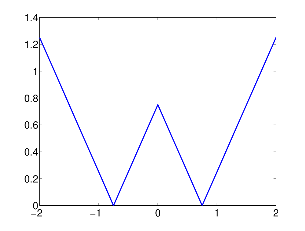
In the simulation, we choose the parameter . The local Lagrangian function can be written as by dropping the terms independent of and is linear in . Figure 4 shows the sectional plot of along -axle, demonstrating that is nonconvex and has local minima.
The inter-agent topologies are given by: is when is odd, and is when is even. It is easy to see that satisfies the periodical strong connectivity assumption II.3.
VI-A1 Simulation 1; the assumption of SD is satisfied
For this numerical simulation, we consider the set of parameters , , , and . Figure 2 shows the surface of the global objective function . The contour, Figure 2, indicates that the set of optimal solutions is a region around . Figure 4 is the sectional plot of along -axle.
From Figures 6–8, one can see that converges to some point . Hence, ; i.e., the assumption of SD is satisfied.
The simulation results are shown in Figures 10 to 10. In particular, Figure 10 (resp. Figure 10) shows the evolution of primal estimates of the primal solution (resp. ). After about 25 iterates, the primal estimates oscillate within a very small region and eventually agree upon the point which coincides with a global optimal solution.
VI-A2 Simulation 2; the assumption of SD is violated
VI-A3 Simulation 3; comparison with gradient-based algorithms
Consider the same set of parameters as in Simulation 1 without including the inequality constraints. The multi-agent interaction topologies are the same. We implement the diffusion gradient algorithm in [18] for this problem. Figures 16 and 16 show that the primal estimates reach the consensus value of after iterates. From Figure 2, it is clear that is not a global optimum. By comparing Figures 10, 10, 16 and 16, one can see that our algorithm is much faster than the diffusion gradient method at the expense of solving a global optimization problem at each iterate.
We also implement the incremental gradient algorithm in [28] for the same set of parameters in Simulation 1 without including inequality constraints. Figure 17 demonstrates that the performance of the incremental gradient method is analogous to the diffusion gradient algorithm; i.e., the estimates are trapped in some local minimum, and the convergence rate is slower than our algorithm.
VI-B Nonconvex quadratic programming
Consider a network of four agents where the topologies are the same as before. The local objective function is and the local constraint function is . In particular, we use the following parameters:
And the local constraint sets are given by
One can see that the sum of is
which is indefinite. We choose for the simulation.
The dual estimates associated with the inequality constraints converge to , , and in Figure 20. One can verify that properties P1 and P2 hold in this case:
The primal estimates converge to , , and in Figures 20 and 20, and the collection of these points consists of a global optimal solution to the approximate problem.
VII Conclusions
We have studied a distributed dual algorithm for a class of multi-agent nonconvex optimization problems. The convergence of the algorithm has been proven under the assumptions that (i) the Slater’s condition holds; (ii) the optimal solution set of the dual limit is singleton; (iii) the network topologies are strongly connected over any given bounded period. An open question is how to address the shortcomings imposed by nonconvexity and multi-agent interactions settings.
References
- [1] A. Abramo, F. Blanchini, L. Geretti, and C. Savorgnan. A mixed convex/nonconvex distributed localization approach for the deployment of indoor positioning services. IEEE Transactions Mobile Computing, 7(11):1325–1337, 2008.
- [2] J.P. Aubin and H. Frankowska. Set-valued analysis. Birkhäuser, 1990.
- [3] D. P. Bertsekas and J. N. Tsitsiklis. Parallel and Distributed Computation: Numerical Methods. Athena Scientific, 1997.
- [4] D.P. Bertsekas. Convex optimization theory. Anthena Scietific, 2009.
- [5] D.P. Bertsekas, A. Nedic, and A. Ozdaglar. Convex analysis and optimization. Anthena Scietific, 2003.
- [6] F. Bullo, J. Cortés, and S. Martínez. Distributed Control of Robotic Networks. Applied Mathematics Series. Princeton University Press, 2009. Available at http://www.coordinationbook.info.
- [7] R.S. Burachik. On primal convergence for augmented Lagrangian duality. Optimization, 60(8):979–990, 2011.
- [8] R.S. Burachik and C.Y. Kaya. An update rule and a convergence result for a penalty function method. Journal of Industrial Management and Optimization, 3(2):381–398, 2007.
- [9] J. Cortés, S. Martínez, T. Karatas, and F. Bullo. Coverage control for mobile sensing networks. IEEE Transactions on Robotics and Automation, 20(2):243–255, 2004.
- [10] J. A. Fax and R. M. Murray. Information flow and cooperative control of vehicle formations. IEEE Transactions on Automatic Control, 49(9):1465–1476, 2004.
- [11] D.Y. Gao, N. Ruan, and H. Sherali. Solutions and optimality criteria for nonconvex constrained global optimization problems with connections between canonical and Lagrangian duality. Journal of Global Optimization, 45(3):474–497, 2009.
- [12] B. Gharesifard and J. Cortés. Distributed strategies for generating weight-balanced and doubly stochastic digraphs. European Journal of Control, 2012. To appear.
- [13] J.-B. Hiriart-Urruty and C. Lemaréchal. Convex Analysis and Minimization Algorithms: Part 1: Fundamentals. Springer, 1996.
- [14] A. Jadbabaie, J. Lin, and A. S. Morse. Coordination of groups of mobile autonomous agents using nearest neighbor rules. IEEE Transactions on Automatic Control, 48(6):988–1001, 2003.
- [15] F. P. Kelly, A. Maulloo, and D. Tan. Rate control in communication networks: Shadow prices, proportional fairness and stability. Journal of the Operational Research Society, 49(3):237–252, 1998.
- [16] A. Nedic and A. Ozdaglar. Approximate primal solutions and rate analysis for dual subgradient methods. SIAM Journal on Optimization, 19(4):1757–1780, 2009.
- [17] A. Nedic and A. Ozdaglar. Distributed subgradient methods for multi-agent optimization. IEEE Transaction on Automatic Control, 54(1):48–61, 2009.
- [18] A. Nedic, A. Ozdaglar, and P.A. Parrilo. Constrained consensus and optimization in multi-agent networks. IEEE Transactions on Automatic Control, 55(4):922–938, 2010.
- [19] R. D. Nowak. Distributed EM algorithms for density estimation and clustering in sensor networks. IEEE Transactions on Signal Processing, 51:2245–2253, 2003.
- [20] P. Oguz-Ekim, J. Gomes, J. Xavier, and P. Oliveira. A convex relaxation for approximate maximum-likelihood 2D source localization from range measurements. In International Conference on Acoustics, Speech, and Signal Processing, pages 2698–2701, 2010.
- [21] R. Olfati-Saber and R. M. Murray. Consensus problems in networks of agents with switching topology and time-delays. IEEE Transactions on Automatic Control, 49(9):1520–1533, 2004.
- [22] A. Olshevsky and J. N. Tsitsiklis. Convergence speed in distributed consensus and averaging. SIAM Journal on Control and Optimization, 48(1):33–55, 2009.
- [23] P.M. Pardalos and S.A. Vavasis. Quadratic programming with one negative eigenvalue is NP-hard. Journal of Global Optimization, 1(1):15–22, 1991.
- [24] B.T. Polyak. A general method for solving extremum problems. Soviet Mathematics Doklady, 3(8):593–597, 1967.
- [25] M. G. Rabbat and R. D. Nowak. Decentralized source localization and tracking. In IEEE International Conference on Acoustics, Speech, and Signal Processing, pages 921–924, May 2004.
- [26] W. Ren and R. W. Beard. Distributed Consensus in Multi-vehicle Cooperative Control. Communications and Control Engineering. Springer, 2008.
- [27] R.T. Rockafellar and R.J.-B Wets. Variational analysis. Springer, 1998.
- [28] S. Sundhar Ram, A. Nedic, and V. V. Veeravalli. Distributed and recursive parameter estimation in parametrized linear state-space models. IEEE Transactions on Automatic Control, 55(2):488–492, 2010.
- [29] L. Xiao, S. Boyd, and S. Lall. A scheme for robust distributed sensor fusion based on average consensus. In Symposium on Information Processing of Sensor Networks, pages 63–70, Los Angeles, CA, April 2005.
- [30] M. Zhu and Martínez. An approximate dual subgradient algorithm for multi-agent non-convex optimization. IEEE Transactions on Automatic Control, 2013. Extended version in http://arxiv.org/abs/1010.2732.
- [31] M. Zhu and S. Martínez. An approximate dual subgradient algorithm for multi-agent non-convex optimization. In IEEE International Conference on Decision and Control, pages 7487–7492, Atlanta, GA, USA, December 2010.
- [32] M. Zhu and S. Martínez. On distributed convex optimization under inequality and equality constraints via primal-dual subgradient methods. IEEE Transactions on Automatic Control, 57:151–164, 2012.