On the stability of the secular evolution of the planar Sun–Jupiter–Saturn–Uranus system
Abstract
We investigate the long time stability of the Sun–Jupiter–Saturn–Uranus system by considering the planar, secular model. Our method may be considered as an extension of Lagrange theory for the secular motions. Indeed, concerning the planetary orbital revolutions, we improve the classical circular approximation by replacing it with a torus which is invariant up to order two in the masses; therefore, we investigate the stability of the elliptic equilibrium point of the secular system for small values of the eccentricities. For the initial data corresponding to a real set of astronomical observations, we find an estimated stability time of years, which is not extremely smaller than the lifetime of the Solar System ( Gyr).
Keywords:
n-body planetary problem , KAM theory , Nekhoroshev theory , normal form methods , exponential stability , Hamiltonian systems , Celestial Mechanics.2010 MSC
Primary: 70F10; Secondary: 37J40 , 37N05 , 70–08 , 70H08.1 Introduction
In this paper we revisit the problem of the stability of the Solar System, at least considering (some of) the major planets, in the light of both Kolmogorov and Nekhoroshev theories. Some aspects are also related to the theory of Lagrange and Laplace on the secular motions of perihelia and nodes of the planetary orbits.
One of our main aims is to point out the major dynamical and computational difficulties that arise in the application of Kolmogorov’s theorem. In view of this, we attempt to apply the Nekhoroshev theory by trying essentially an extension of Lagrange theory. Although the final results appear to be interesting, our conclusion will be that further and more refined investigations are needed. We consider indeed the present paper as the beginning of a more comprehensive study of systems with more than two planets in the framework of perturbation methods related to the theories above.
In 1954 Kolmogorov announced his celebrated theorem on the persistence under small perturbation of quasi periodic motions on invariant tori of an integrable Hamiltonian systems (see [30]). The relevance of that result for the problem of stability of the Solar System was pointed out by Kolmogorov himself, and later emphasized in the subsequent papers of Moser (see [48]) and Arnold (see [1]). The three papers mentioned above marked the beginning of the so called KAM theory.
However the actual applicability of Kolmogorov’s theorem to the planetary system encounters two major difficulties, namely: (i) the degeneracy of the Keplerian motion, and (ii) the extremely restrictive assumptions on the smallness of the perturbation.
The former difficulty is related to the elliptic form of the Keplerian orbits. Indeed a system including a central body (a star) and planets, after elimination of the known first integrals, has degrees of freedom, while only actions appear in the Keplerian part of the Hamiltonian. The way out proposed by Arnold, and inspired by the approach of Lagrange and Laplace, was to introduce in the proof two separate time scales for the orbital motion and for the secular evolution of the perihelia and of the nodes (see [2] and its recent extension in [9]). Such an approach has been successfully extended to the -body planetary systems thanks to the work done by Herman and Féjoz (see [11]).
Attacking the second difficulty (i.e., the unrealistic requirements on the smallness of masses, eccentricities and inclinations of the planets) with purely analytical methods seems to be unrealistic. However, some positive results could be attained using computer algebra. This means that we explicitly perform a few perturbation steps, thus getting an approximation of the wanted invariant torus which is good enough to allow us to apply analytical methods. Such an approach (also implementing interval arithmetic) allowed some authors to rigorously prove the existence of KAM tori for some interesting problems in Celestial Mechanics (see, e.g., [6], [7], [8], [44] and [12]). However, all these works consider models having just two degrees of freedom. This because increasing the number of independent variables makes the explicit calculation of perturbation steps a big challenge, due to the dramatic increase of the number of coefficients to be calculated, so that a sufficiently good initial approximation of an invariant torus is hardly obtained. For what concerns problems with more than two degrees of freedom, in a few cases only the availability of an algorithmic version of Kolmogorov’s theorem (see [3], [17] and [18]) allowed us to obtain a good approximation of the invariant tori, although this approach is not yet sufficient for a fully rigorous application of the theory. For instance, the constructed solution on a KAM torus has been successfully compared with the real motion of the Sun–Jupiter–Saturn system, which can be represented by a model with degrees of freedom (see [46] for all details). Moreover our recent work focuses on a first study of the long time stability in a neighborhood of such KAM torus (see [19]).
Besides the technical difficulty, the results of the numerical explorations have raised some doubts concerning the applicability of Kolmogorov theory to the major bodies of our planetary system, namely the Sun and the so called Jovian planets, i.e. Jupiter, Saturn, Uranus and Neptune, hereafter we will refer to this model as the SJSUN problem. Indeed, the motion of such planetary subsystem has been shown to be chaotic by Sussman and Wisdom (see [58]). Murray and Holman provided such an enlightening explanation of this phenomenon, that we think it is helpful to briefly summarize some of their results as follows (see [49] for completeness).
- (a)
The chaoticity of the Jovian planets appears to be due to the overlap of some resonances involving three or four bodies. An example is given by the resonances
where stands for the mean motion frequency of the -th planet, means the (secular) frequency of its perihelion argument and the indexes refer to Jupiter, Saturn and Uranus, respectively. In fact, during the planetary motion each angle corresponding to the resonances above moves from libration to rotation and viceversa. Many other resonances analogous to the previous ones are located in the vicinity of the real orbit of the SJSUN system, some of them involving also Neptune and the frequencies related to the longitudes of the nodes.
- (b)
The time needed by these resonances to eject Uranus from the Solar System is roughly evaluated to be about years.
- (c)
By moving the initial semi-major axis of Uranus in the range – AU one observes some regions that look filled by quasi-periodic ordered motions and other regions that are weakly chaotic, i.e., with a Lyapunov time ranging between and years. All the main resonances acting in this region involve the linear combination among the mean motion frequencies of Jupiter, Saturn and Uranus.
- (d)
The result (c) qualitatively persists also for the planar SJSUN system or when the influence of Neptune is neglected.
- (e)
Conversely, no chaotic motions are detected in the planar system including the Sun, Jupiter, Saturn and Uranus (hereafter, SJSU for shortness) for the same initial values of the semi-major axis of Uranus considered at point (c). This suggests that the resonances described at point (a) affect observable regions only when combined with some effects induced by Neptune or by the mutual inclinations.
By the way, we note that the resonances involving the linear combination are clearly related to the approximate ratio and between the orbital motion of Jupiter and Saturn and of Jupiter and Uranus, respectively. Similarly, the ratio between Uranus and Neptune appears also to be relevant (historically, this helped Le Verrier to predict the existence and the location of Neptune). The low order of the latter quasi-resonance may explain why the influence of Neptune induces some chaotic behavior, as pointed out in (d) and (e) above. An overlapping of resonances involving the linear combination among the mean motion frequencies of all the Jovian planets has been actually detected in a small region including their orbits; this has been made possible by a combined use of some refined numerical investigation methods (see [22] and [23]). Moreover, the coexistence of quasi-periodic and chaotic motions in a neighborhood of the real initial conditions (already pointed out in the remark (c) above) has been recently shown to be extremely complicated (see [24] and [25]).
The weak chaos in the motion of the Jovian planets (see, e.g., [29] for a review on this topic) makes somehow hopeless the task of describing their long-term evolution by a quasi-periodic approximation, as it is provided by the KAM theory. Therefore it appears to be more natural to look for exponential stability as assured by Nekhoroshev theory (see [50] and [51]). Indeed the theorem of Nekhoroshev applies to an open set of initial conditions, and states that the stability time increases exponentially with the inverse of the perturbation parameter. Our aim is to investigate whether the SJSU system may remain close to its current conditions for a time that exceeds the lifetime of the system itself; e.g., in our case the age of the Universe, which is estimated to be years, could be enough. We stress that the rather long time reported in (b) concerning the possible dissolution of the SJSUN system seems to support our hope. The approach based on Nekhoroshev theory has been applied during the last decades to the case of the Trojan asteroids, producing realistic results (see, e.g., [21], [56], [10] and [42]). Concerning the SJSUN system, we expect that a combination of both the KAM and the Nekhoroshev theory could prove that the motion remains close to an invariant torus for very long times (see [47] and [19]).
In the present paper, we restrict our attention to the SJSU planar system, due to the huge computational difficulties one encounters during the expansion of the Hamiltonian. Indeed, a rather long preliminary work is necessary in order to give the Hamiltonian a convenient form for starting more standard perturbation methods (see [44], [45] and [46]). We devote sects. 2 and 3.1 to this part of the problem.
Furthermore, in the line of Lagrange theory, we focus only on the secular part of the Hamiltonian, which is derived in subsect. 3.2. Let us emphasize that all along both sects. 2 and 3 we pay a special attention to include all the relevant terms related to the three-body mean motion quasi-resonance in view of the remarks reported at points (a) and (c) above).
The secular system turns out to have the form of a perturbed system of harmonic oscillators. Let us recall that the stability of its equilibrium point could be investigated using the theorem of Dirichlet. In fact, we can use as Lyapunov function either the secular Hamiltonian or another integral of motion that is related to the total angular momentum. For planar systems, the secular Hamiltonian is a first integral with a minimum corresponding to the case where all orbits are circular. This is enough to ensure that the eccentricities remain bounded forever if their initial values are small enough. Indeed, Lagrange and Laplace actually proved Dirichlet’s theorem for the special case of the secular part of the spatial planetary system, by using the third component of the total angular momentum as Lyapunov function. However, a chaotic evolution inside the stability domain is not excluded by their approach: the eccentricity or the inclination of a planet could increase up to the maximum value allowed. This is in contrast with the features of the motion of the Jovian planets, which have been discussed above. Thus, even when we limit ourselves to the study of the secular planar case, we think that it is useful to proceed by investigating the stability into the light of Nekhoroshev theory, since it provides also the information that the eccentricities of the planets essentially have a quasi-periodic behavior, apart from the very small contribution induced by the high order perturbing terms. Moreover, our approach can be extended to more refined models including the dependency on the mean motion angles. The study of the secular Hamiltonian by using the Nekhoroshev theory is worked out in sect. 4.
Finally, sect. 5 is devoted to the conclusions.
2 Classical expansion of the planar planetary Hamiltonian
Let us consider four point bodies , with masses , mutually interacting according to Newton’s gravitational law. Hereafter the indexes will correspond to Sun, Jupiter, Saturn and Uranus, respectively.
Let us now recall how the classical Poincaré variables can be introduced so to perform a first expansion of the Hamiltonian around circular orbits, i.e., having zero eccentricity. We basically follow the formalism introduced by Poincaré (see [52] and [53]; for a modern exposition, see, e.g., [40] and [41]). We remove the motion of the center of mass by using heliocentric coordinates , with . Denoting by the momenta conjugated to , the Hamiltonian of the system has degrees of freedom, and reads
| (1) |
where
The plane set of Poincaré’s canonical variables is introduced as
|
|
(2) |
for , where and are the semi-major axis, the eccentricity, the mean anomaly and the perihelion longitude, respectively, of the -th planet. One immediately sees that both and are of the same order of magnitude as the eccentricity .
Using Poincaré’s variables (2), the Hamiltonian can be rearranged so that one has
| (3) |
where , . Here, the small dimensionless parameter , , has been introduced in order to highlight the different size of the terms appearing in the Hamiltonian. Let us remark that the time derivative of each coordinate is but in the case of the angles . Therefore, according to the common language in Celestial Mechanics, in the following we will refer to and to their conjugate actions as the fast variables, while will be called secular variables.
We proceed now by expanding the Hamiltonian (3) in order to construct the first basic approximation of Kolmogorov’s normal form. We pick a value for the fast actions and perform a translation defined as
| (4) |
This is a canonical transformation that leaves the coordinates , and unchanged. The transformed Hamiltonian can be expanded in power series of around the origin. Thus, forgetting an unessential constant we rearrange the Hamiltonian of the system as
| (5) |
where the functions are homogeneous polynomials of degree in the actions and of degree in the secular variables . The coefficients of such homogeneous polynomials do depend analytically and periodically on the angles . The terms of the Keplerian part are homogeneous polynomials of degree in the actions , the explicit expression of which can be determined in a straightforward manner. In the latter equation the term which is both linear in the actions and independent of all the other canonical variables (i.e., ) has been separated in view of its relevance in perturbation theory, as it will be discussed in the next section. We also expand the coefficients of the power series in Fourier series of the angles . The expansion of the Hamiltonian is a traditional procedure in Celestial Mechanics. We work out these expansions for the case of the planar SJSU system using a specially devised algebraic manipulation. The calculation is based on the approach described in sect. 2.1 of [44], which in turn uses the scheme sketched in sect. 3.3 of [55].
| Jupiter () | Saturn () | Uranus () | |
|---|---|---|---|
The reduction to the planar case is performed as follows. We pick from Table IV of [57] the initial conditions of the planets in terms of heliocentric positions and velocities at the Julian Date . Next, we calculate the corresponding orbital elements with respect to the invariant plane (that is perpendicular to the total angular momentum). Finally we include the longitudes of the nodes (which are meaningless in the planar case) in the corresponding perihelion longitude and we eliminate the inclinations by setting them equal to zero. The remaining initial values of the orbital elements are reported in Table 1.
Having determined the initial conditions we come to determining the average values of the semi-major axes during the evolution. To this end we perform a long-term numerical integration of Newton’s equations starting from the initial conditions related to the data reported in Table 1. After having computed , we determine the values via the first equation in (2). This allows us to perform the expansion (5) of the Hamiltonian as a function of the canonical coordinates . In our calculations we truncate the expansion as follows. (a) The Keplerian part is expanded up to the quadratic terms. The terms include: (b1) the linear terms in the actions , (b2) all terms up to degree in the secular variables , (b3) all terms up to the trigonometric degree with respect to the angles . Our choice of the limits will be fully motivated in the next section. However, let us anticipate here that we focus our attention on the features of our final secular model: we aim to include there as much as possible of the effects of the quasi-resonances involving the mean motion frequencies of the three planets the impact of which on the dynamics has been discussed in the introduction. Thus, we push our expansion in and as high as possible, although a low order truncation in is used (see, e.g., [28] for some standard evaluation criteria).
3 The secular model
We look now for a good description of the secular dynamics. A straightforward method would be to include in the unperturbed Hamiltonian also the average of the perturbation over the fast angles. However, it has been remarked by Robutel (see [54]) that the frequencies of the quasi-periodic flow given by this secular Hamiltonian (often called of order one in the masses) are quite different from the true ones. The reason lies in the effect of the mean motion quasi-resonance . Therefore we look for an approximation of the secular Hamiltonian up to order two in the masses (see, e.g., [38], [39], [54], [44], [31] and [43]). To this end we follow the approach in [46], carrying out two “Kolmogorov-like” normalization steps in order to eliminate the main perturbation terms depending on the fast angles . We concentrate our attention on the quasi-resonant angles , and , which are the most relevant ones for the dynamics. Our aim is to replace the orbit with zero eccentricity with a quasi-periodic one that takes into account the effect of such quasi-resonances up to the second order in the masses. The procedure is a little cumbersome, and requires two main steps that we describe in the next two subsections.
3.1 Partial reduction of the perturbation
We emphasize that the Fourier expansion of the Hamiltonian (5) is generated just by terms due to two-body interactions, and so harmonics including more than two fast angles cannot appear. Thus, at first order in the masses only harmonics with the quasi-resonant angles and do occur. Actually, harmonics with the quasi-resonant angle are generated by the first Kolmogorov-like transformation, but are of second order in the masses, and should be removed by the second Kolmogorov-like transformation described in the next section.
Let us go into details. We denote by the Fourier expansion of a function truncated so as to include only its harmonics satisfying the restriction , being . We also denote by the average with respect to the angles , , . The canonical transformations are using the Lie series algorithm (see, e.g., [14]).
We set and transform the Hamiltonian (5) as with the generating function determined by solving the equation
| (6) |
Notice that, by definition, , which assures that equation (6) can be solved provided the frequencies are not resonant up to order , as it actually occurs in our planar model of the SJSU system.
The Hamiltonian has the same form of in (5), with the functions replaced by new ones, that we denote by , generated by the expanding the Lie series and by gathering all the terms having the same degree both in the fast actions and in the secular variables.
Now we perform a second canonical transformation , where the generating function (which is linear with respect to ) is determined by solving the equation
| (7) |
Again, the Hamiltonian can be written in a form similar to (5), namely
| (8) |
where the new functions are calculated as previously explained for . Moreover, they still have the same dependence on their arguments as in (5).
If terms of second order in are neglected, then the Hamiltonian possesses the secular -dimensional invariant torus and . Thus, in a small neighborhood of the origin of the fast actions and for small eccentricities the solutions of the system with Hamiltonian differ from those of its average by a quantity . In this sense the average of the Hamiltonian (8) approximates the real dynamics of the secular variables up to order two in the masses, and due to the choice takes into account the quasi-resonances between Jupiter and Saturn and between Jupiter and Uranus.
In this part of the calculation we produce a truncated series which is represented as a sum of monomials
The truncated expansion of contains such monomials. We truncate our expansion at degree 16 in the fast angles and at degree 18 in the slow variables (we shall justify this choice at the end of the next section).
3.2 Second approximation and reduction to the secular Hamiltonian
The huge number of coefficients determined till now does not allow us to continue by keeping all of them. Therefore, in view that we plan to consider the secular system, we perform a partial average by keeping only the main terms that contain the quasi-resonant angle . More precisely, we first consider the reduced Hamiltonian
| (9) |
namely we set , which results in replacing the orbit having zero eccentricity with a close invariant torus of the unperturbed Hamiltonian, and average by removing all the Fourier harmonics depending on the angles. Next, we select in the Fourier harmonics that contain the wanted quasi-resonant angle and add them to the Hamiltonian (9). Finally, we perform on the resulting Hamiltonian the second Kolmogorov-like step. With more detail, this is the procedure, which is an adaptation of a scheme already used in [44].
For we select the quasi-resonant terms
|
|
(10) |
Actually, this means that in our expression we just remove all monomials but the ones containing the wanted quasi-resonant angle. Using the selected terms we determine a generating function by solving the equation
| (11) |
Here we make the calculation faster by keeping only terms up to degree in , this allows us to keep the more relevant quasi-resonant contributions. Then, still following the procedure outlined in [44], we calculate only the interesting part of the transformed Hamiltonian , namely we keep in the transformation only the part which is independent of all the fast variables . This produces the secular Hamiltonian , which satisfies the formal equation , where
|
|
(12) |
Here, we denoted by and the terms of the Poisson bracket involving only the derivatives with respect the variables and , respectively.
The Hamiltonian so constructed is the secular one, describing the slow motion of eccentricities and perihelia. In view of D’Alembert rules contains only terms of even degree and so the lowest order significant term has degree 2 (see, e.g., [53] and also [26]–[27] for a modern approach, suitable for evaluating the non-zero coefficients). We have determined the power series expansion of the Hamiltonian up to degree 18 in the slow variables. In order to allow a comparison with other expansions, we reported our results up to degree 4 in in appendix A.
We close this section with a few remarks which justify our choice of the truncation orders. The limits on the expansions in the fast actions have been illustrated at points (a) and (b1) at the end of section 2, and they are the smallest ones that are required in order to make the Kolmogorov-like normalization procedure significant. Since we want to keep the quasi-resonant angles , and , we set the truncation order for Fourier series to , which is enough. The choice to truncate the expansion at degree in the secular variables is somehow subtler. In view of D’Alembert rules the harmonics and have coefficients of degree at least 3 and 6, respectively, in the secular variables. Furthermore, the quasi-resonant angle does not appear initially in the Hamiltonian, but is generated by Poisson bracket between the harmonics and , which produces monomials of degree in . Therefore, we decided to calculate the generating functions and up to degree (recall equations (6) and (7)). Finally, in the second Kolmogorov-like step we want to keep the secular terms generated by the harmonic , which are produced by Poisson bracket between monomials containing precisely this harmonic, and then the result has maximum degree in . This explains the final truncation order for the slow variables.
4 Stability of the secular Hamiltonian model
The lowest order approximation of the secular Hamiltonian , namely its quadratic term, is essentially the one considered in the theory first developed by Lagrange (see [32]) and furtherly improved by Laplace (see [35], [36] and [37]) and by Lagrange himself (see [33], [34]). In modern language, we say that the origin of the reduced phase space (i.e., ) is an elliptic equilibrium point (for a review using a modern formalism, see sect. 3 of [4], where a planar model of our Solar System is considered).
It is well known that (under mild assumptions on the quadratic part of the Hamiltonian which are satisfied in our case) one can find a linear canonical transformation which diagonalizes the quadratic part of the Hamiltonian, so that we may write in the new coordinates as
| (13) |
where are the secular frequencies in the small oscillations limit and is a homogeneous polynomial of degree in . The calculated values of in our case are reported in Table 2.
Thus, we are led to study the stability of the equilibrium for the Hamiltonian (13). As remarked in the introduction, perpetual stability in a neighborhood of the equilibrium is ensured by applying Dirichlet’s theorem. We can do it in two ways. Since all frequencies have the same sign (that is negative in our case), we can use as Lyapunov function; actually, a very rough evaluation of the size of the stability neighborhood gives us a value of the radius that is about times the distance (from the origin) of the actual initial data of the planets. Such an estimate should certainly be improved by a more accurate calculation, i.e., by determining the stationary points of a function in 6 variables. A second alternative approach focuses on the constant of motion related to the total angular momentum. In fact, is a first integral for the initial Hamiltonian described in (3). Thus, one can use as Lyapunov function the average of the angular momentum , when it is expressed as a function of the new secular canonical coordinates . However, we emphasize that the Dirichlet theory does not apply to a complete planetary system, that is not averaged with respect to the mean motion angles. Thus, as said in the introduction, we think it is more interesting to investigate the stability of the equilibrium in the light of Nekhoroshev theory, in view of its possible extension to more refined models.
4.1 Birkhoff’s normal form
Following a quite standard procedure we proceed to construct the Birkhoff’s normal form for the Hamiltonian (13) (see [5]; for an application of Nekhoroshev theory see, e.g., [13]). This is a well known matter, thus we limit our exposition to a short sketch adapted to the present context.
The aim is to give the Hamiltonian the normal form at order
| (14) |
where
| (15) |
are the actions of the system, and for is a homogeneous polynomial of degree in and in particular it is zero for odd . The un-normalized reminder terms , where , are homogeneous polynomials of degree in .
We proceed by induction. Assume that the Hamiltonian is in normal form up to a given order , which is trivially true for , and determine a generating function and the normal form term , by solving the equation
| (16) |
Using the algorithm of Lie series transform, we can write the new Hamiltonian as . It is not difficult to show that has a form analogous to that written in (14) with new functions of degree (where ) and the normal form part ending with , which is equal to zero if is even (see, e.g., [16]). As usual when using the Lie series methods, we denote by the new coordinates, so that the normal form possesses the approximate first integrals given by (15). By the way, the algorithm can be iterated up to the step provided that the non-resonance condition
| (17) |
is fulfilled.
4.2 Study of the stability time
It is well known that Birkhoff’s normal form at any finite order is convergent in some neighborhood of the origin, but the analyticity radius shrinks to zero when . Thus, the best one can do is to look for stability for a finite but long time. We use the algorithm reported in [20], that we describe here.
Let us pick three positive numbers and consider a polydisk with center at the origin of defined as
being a parameter. Let , and let be the initial point of an orbit, so that one has . Therefore, there is such that for we have , and so also . We call the estimated stability time, and our aim is to give a good estimate of it.
The key remark is that one has
| (18) |
which holds true for an arbitrary normalization order . This means that the time derivative of is small, being , so that the time may grow very large. The basis of Nekhoroshev theory is that one can choose an optimal value of as a function of letting it to get larger and larger when , so that grows faster than any power of . Here we give this argument an algorithmic form, thus producing an explicit estimate of .
Let us write a homogeneous polynomial of degree as
where the multiindex notation has been used. We define the quantity as
| (19) |
We claim that for one has
| (20) |
The estimate is checked as follows. In the plane consider a disk with radius . Then inside the disk the inequality holds true. In fact, after having set , one can easily check that . It is then straightforward to verify that for a monomial of degree one has
The wanted inequality is just the sum of the contributions of all monomials.
Using (20) and (18) we can estimate
| (21) |
for and with some . In fact, after having set smaller than the convergence radius of the remainder series (where ), the above inequality is true for some . In our calculation we set .
We come now to the calculation of the estimated stability time. Since , we have and, in view of inequality (21), also
Thus a majorant of the function is given by the solution of the equation . Setting as the initial value we conclude that for all , where
| (22) |
The latter estimate holds true for arbitrary normalization order . Therefore we select an optimal order by looking for the maximum over of , thus getting
| (23) |
This is the best estimate of the stability time given by our algorithm.
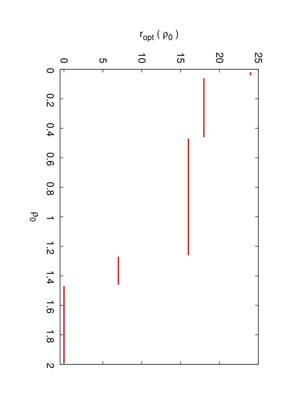

4.3 Application to the SJSU system
We apply the algorithm of the previous section to the secular Hamiltonian by explicitly performing the construction of Birkhoff’s normal form up to order . Meanwhile also the first term of the remainder has been stored, so that the estimate for is provided.
The calculation of the estimated stability time is performed by setting
| (24) |
These values have been calculated as where are the initial data reported in table 2, so that the initial point is on the border of the polydisk with .
Finally we proceed to calculating the optimal normalization order and the estimated stability time as functions of in an interval such that the optimal normalization order produced by our algorithm is less than . The results are reported in fig. 1. The fast increase of the time when decreases is evident from the graph. We also remark that for , which corresponds to the initial data for the planets, the normalization order is already . This shows that the mechanism of long time stability is already active. The estimated time with our algorithm is about years for . This seems to be quite short both with respect to the age of the Solar System (which is estimated to be years) and with respect to the numerical indications ( years). We shall comment on this point in the next section.
5 Conclusions and outlooks
In the framework provided by the Nekhoroshev’s theorem, the present paper describes the first attempt to study the stability of a realistic model with more than two planets of our Solar System. As remarked at the end of the previous section we are not yet able to prove the stability for a time comparable to the age of our planetary system, even restricting ourselves to consider just the secular part of a planar approximation including the Sun, Jupiter, Saturn and Uranus. Nevertheless, we think that our result is meaningful in that it indicates that the phenomenon of exponential stability in Nekhoroshev sense may play an effective role for the Solar System, at least for the biggest planets. On the other hand, we stress that our result is not dramatically far from the goal of proving stability for the age of the Solar System: such a time is reached for . By the way, it may be worth to note that a similar result, with the same value of the radius, has been found in [20] where the spatial problem for the Sun–Jupiter–Saturn system is considered. Such a value of appears to be not so small, especially if one recalls the rough estimates based on the first purely analytical proofs of the KAM theorem: in order to apply them to some model of our planetary system, the Jupiter mass should be smaller than that of a proton. Improvements are surely possible, and the relatively short history of the applications of the Nekhoroshev type estimates to Celestial Mechanics has shown definitely more remarkable improvements than the one required here (e.g., compare [15] with [21]).
Some drawbacks are immediately evident. The most relevant one is that the estimate in (22) actually assumes that the perturbation constantly forces the worst possible evolution. This is clearly pessimistic, and justifies the striking difference with respect to the indication given by the numerical integrations. On the other hand, general perturbation method are essentially based on estimates that are often very crude. The explicit calculation of normal forms and related quantities allows us to significantly improve our results, but the price is either a bigger and bigger computer power or more and more refined methods.
The natural question is whether there is a way to improve the present result. Our approach suggests that a better approximation of the true orbit could help a lot. This can be obtained, e.g., by first establishing the existence of a KAM torus close to the initial conditions of the planets, and then proving the stability in Nekhoroshev sense in a neighborhood of the torus that contains the initial data. Such an approach has been attempted in [19] for the Sun–Jupiter–Saturn case considering the full system, i.e., avoiding the approximation of the secular model. In that case the number of coefficients to be handled is so huge that the calculation can actually be performed only by introducing strong truncations on the expansions; this might artificially improve the results. Thus, some new idea is necessary, and this will be work for the future.
Acknowledgments
The authors have been supported by the research program “Dynamical Systems and applications”, PRIN 2007B3RBEY, financed by MIUR. M.S. has been partially supported also by the research program “Studi di Esplorazione del Sistema Solare”, financed by ASI.
Appendix A Expansion of the secular Hamiltonian of the planar SJSU system up to order 2 in the masses and 4 in eccentricities
Our secular model is represented by the Hamiltonian , which is defined in (12). Here, we limit ourselves to report the expansion of up to degree in . Therefore, as a consequence of the D’Alembert rules, the terms related to the quasi-resonance do not give any contribution to the coefficients listed below. Thus, the following expansion of the rhs of (12) actually takes into account just (recall that contains just terms of even degree in its variables ). The calculation of the functions and is performed how it has been explained in subsect. 3.1.
References
- [1] V. Arnold, Proof of a theorem of A.N. Kolmogorov on the invariance of quasi–periodic motions under small perturbations of the Hamiltonian, Usp. Mat. Nauk 18 (1963a). Russ. Math. Surv., 18, 9 (1963).
- [2] V. Arnold, Small denominators and problems of stability of motion in classical and celestial mechanics, Usp. Mat. Nauk 18 (1963b). Russ. Math. Surv. 18 6 (1963).
- [3] G. Benettin, L. Galgani, A. Giorgilli, J. Strelcyn, A Proof of Kolmogorov’s Theorem on Invariant Tori Using Canonical Transformations Defined by the Lie method, Nuovo Cimento 79 (1984) 201–223.
- [4] L. Biasco, L. Chierchia, E. Valdinoci, N–dimensional elliptic invariant tori for the planar (N+1)–body problem, SIAM Journal on Mathematical Analysis 37 (2006) 1560–1588.
- [5] G. Birkhoff, Dynamical systems, New York, 1927.
- [6] A. Celletti, Construction of librational invariant tori in the spin–orbit problem, J. of Applied Math. and Physics (ZAMP) 45 (1994) 61–80.
- [7] A. Celletti, L. Chierchia, On the stability of realistic three–body problems, Comm. Math. Phys. 186 (1997) 413–449.
- [8] A. Celletti, L. Chierchia, KAM stability and Celestial Mechanics, Memoirs of AMS 187 (2007).
- [9] L. Chierchia, G. Pinzari, Properly degenerate KAM theory (following V.I. Arnold), DCDS-S (2009). In press.
- [10] C. Efthymiopoulos, Z. Sándor, Optimized Nekhoroshev stability estimates for the Trojan asteroids with a symplectic mapping model of co–orbital motion, Mon. Not. R. Astron. Soc. 364 (2005) 253–271.
- [11] J. Fejoz, Démonstration du “théorème d’Arnold” sur la stabilité du système planétaire (d’après Michael Herman), Ergodic Theory Dyn. Sys. 24 (2005) 1521–1582.
- [12] F. Gabern, A. Jorba, U. Locatelli, On the construction of the Kolmogorov normal form for the Trojan asteroids, Nonlinearity 18 (2005) 1705–1734.
- [13] A. Giorgilli, Rigorous results on the power expansions for the integrals of a Hamiltonian system near an elliptic equilibrium point, Ann. Inst. H. Poincaré 48 (1988) 423–439.
- [14] A. Giorgilli, Quantitative methods in classical perturbation theory, in: From Newton to chaos: modern techniques for understanding and coping with chaos in N–body dynamical systems, Nato ASI school, A.E. Roy e B.D., 1995.
- [15] A. Giorgilli, A. Delshams, E. Fontich, L. Galgani, C. Simó, Effective stability for a Hamiltonian system near an elliptic equilibrium point, with an application to the restricted three body problem, J. Diff. Eqs. 20 (1989). Steves eds., Plenum Press, New York (1995).
- [16] A. Giorgilli, L. Galgani, Formal integrals for an autonomus Hamiltonian system near an elliptic equilibrium point, Celestial Mechanics and Dynamical Astronomy 17 (1978) 267–280.
- [17] A. Giorgilli, U. Locatelli, Kolmogorov theorem and classical perturbation theory, J. of App. Math. and Phys. (ZAMP) 48 (1997a) 220–261.
- [18] A. Giorgilli, U. Locatelli, On classical series expansion for quasi–periodic motions, MPEJ 3 (1997b) 1–25.
- [19] A. Giorgilli, U. Locatelli, M. Sansottera, Kolmogorov and Nekhoroshev theory for the problem of three bodies, Celestial Mechanics and Dynamical Astronomy 104 (2009) 159–173.
- [20] A. Giorgilli, U. Locatelli, M. Sansottera, Su un’estensione della teoria di Lagrange per i moti secolari, Rendiconti dell’Istituto Lombardo Accademi di Scienze e Lettere (2010). To appear.
- [21] A. Giorgilli, C. Skokos, On the stability of the Trojan asteroids, Astron. Astroph. 317 (1997) 254–261.
- [22] M. Guzzo, The Web of Three-Planet Resonances in the Outer Solar System, Icarus 174 (2005) 273–284.
- [23] M. Guzzo, The Web of Three-Planet Resonances in the Outer Solar System. II. A Source of Orbital Instability for Uranus and Neptune, Icarus 181 (2006) 475–485.
- [24] W. Hayes, Is the outer Solar System chaotic?, Nature Physics 3 (2007) 689–691.
- [25] W. Hayes, Surfing on the edge: chaos versus near-integrability in the system of Jovian planets, Monthly Not. Royal Astr. Soc. 386 (2008) 295–306.
- [26] K. Kholshevnikov, D’Alembertian Functions in Celestial Mechanics, Astronomy Reports 41 (1997) 135–142.
- [27] K. Kholshevnikov, The Hamiltonian in the Planetary or Satellite Problem as a D’Alembertian Function, Astronomy Reports 45 (2001) 577–579.
- [28] K. Kholshevnikov, A. Greb, E. Kuznetsov, The Expansion of the Hamiltonian of the Two-Planetary Problem into a Poisson Series in All Elements: Estimation and Direct Calculation of Coefficients, Solar System Research 36 (2001) 68–79.
- [29] K. Kholshevnikov, E. Kuznetsov, Review of theWorks on the Orbital Evolution of Solar System Major Planets, Solar System Research 41 (2007) 291–329.
- [30] A. Kolmogorov, Preservation of conditionally periodic movements with small change in the Hamilton function, Dokl. Akad. Nauk SSSR 98 (1954). Engl. transl. in: Los Alamos Scientific Laboratory translation LA-TR-71-67; reprinted in: Lecture Notes in Physics, 93.
- [31] E. Kuznetsov, K. Kholshevnikov, Dynamical Evolution of Weakly Disturbed Two-Planetary System on Cosmogonic Time Scales: the Sun–Jupiter–Saturn System, Solar System Research 40 (2006) 239–250.
- [32] J. Lagrange, Sur l’altération des moyens mouvements des planètes, Mem. Acad. Sci. Berlin 199 (1776). Oeuvres complètes, VI, 255, Gauthier–Villars, Paris (1869).
- [33] J. Lagrange, Théorie des variations séculaires des éléments des planètes. première partie contenant les principes et les formules générales pour déterminer ces variations, Nouveaux mémoires de l Académie des Sciences et Belles–Lettres de Berlin (1781). Oeuvres complètes, V, 125–207, Gauthier–Villars, Paris (1870).
- [34] J. Lagrange, Théorie des variations séculaires des éléments des planètes. Seconde partie contenant la détermination de ces variations pour chacune des planètes pricipales, Nouveaux mémoires de l Académie des Sciences et Belles–Lettres de Berlin (1782). Oeuvres complètes, V, 211–489, Gauthier–Villars, Paris (1870).
- [35] P. Laplace, Mémoire sur les solutions particulières des équations différentielles et sur les inégalités séculaires des planètes (1772). Oeuvres complètes, IX, 325, Gauthier–Villars, Paris (1895).
- [36] P. Laplace, Mémoire sur les inégalités séculaires des planètes et des satellites, Mem. Acad. royale des Sci. de Paris (1784). Oeuvres complètes, XI, 49, Gauthier–Villars, Paris (1895).
- [37] P. Laplace, Théorie de Jupiter et de Saturne, Mem. Acad. royale des Sci. de Paris (1785). Oeuvres complètes, XI, 164, Gauthier–Villars, Paris (1895).
- [38] J. Laskar, Secular evolution over 10 million years, Astronomy and Astrophysics 198 (1988) 341–362.
- [39] J. Laskar, A numerical experiment on the chaotic behaviour of the solar system, Nature 338 (1989a) 237–238.
- [40] J. Laskar, Systèmes de variables et éléments, in: D. Benest, C. Froeschlé (Eds.), Les Méthodes modernes de la Mécanique Céleste, Editions Frontières, 1989b, pp. 63–87.
- [41] J. Laskar, P. Robutel, Stability of the Planetary Three–Body Problem — I. Expansion of the Planetary Hamiltonian, Celestial Mechanics and Dynamical Astronomy 62 (1995) 193–217.
- [42] C. Lhotka, C. Efthymiopoulos, R. Dvorak, Nekhoroshev stability at L4 or L5 in the elliptic–restricted three–body problem — application to the Trojan asteroids, Mon. Not. R. Astron. Soc. 384 (2008) 1165–1177.
- [43] A. Libert, J. Henrard, Analytical study of the proximity of exoplanetary systems to mean–motion resonances, Astronomy and Astrophysics 461 (2007) 759–763.
- [44] U. Locatelli, A. Giorgilli, Invariant tori in the secular motions of the three–body planetary systems, Celestial Mechanics and Dynamical Astronomy 78 (2000) 47–74.
- [45] U. Locatelli, A. Giorgilli, Construction of the Kolmogorov’s normal form for a planetary system, Regular and Chaotic Dynamics 10 (2005) 153–171.
- [46] U. Locatelli, A. Giorgilli, Invariant tori in the Sun–Jupiter–Saturn system, DCDS-B 7 (2007) 377–398.
- [47] A. Morbidelli, A. Giorgilli, Superexponential stability of KAM tori, J. Stat. Phys. 78 (1995) 1607–1617.
- [48] J. Moser, On invariant curves of area–preserving mappings of an annulus, Nachr. Akad. Wiss. Gött., II Math. Phys. Kl 1962 (1962) 1–20.
- [49] N. Murray, M. Holman, The Origin of Chaos in Outer Solar System, Science 283 (1999) 1877–1881.
- [50] N. Nekhoroshev, Exponential estimates of the stability time of near–integrable Hamiltonian systems, Russ. Math. Surveys 32 (1977).
- [51] N. Nekhoroshev, Exponential estimates of the stability time of near–integrable Hamiltonian systems, 2, Trudy Sem. Petrovs. 5 (1979).
- [52] H. Poincaré, Les méthodes nouvelles de la Mécanique Céleste, Gauthier–Villars, Paris, 1892. Reprinted by Blanchard (1987).
- [53] H. Poincaré, Leçons de Mécanique Céleste, tomes I–II, Gauthier–Villars, Paris, 1905.
- [54] P. Robutel, Contribution à l’étude de la stabilité du problème planetaire des trois corps, Ph.D. thesis, Observatoire de Paris, 1993.
- [55] P. Robutel, Stability of the Planetary Three–Body Problem — II. KAM Theory and Existence of Quasiperiodic Motions, Celestial Mechanics and Dynamical Astronomy 62 (1995) 219–261.
- [56] C. Skokos, A. Dokoumetzidis, Effective stability of the Trojan asteroids, Astron. Astroph. 367 (2001) 729–736.
- [57] E. Standish, JPL Planetary and Lunar Ephemerides, DE405/LE405, Jet Propulsion Laboratory – Interoffice memorandum IOM 312.F – 98 – 048 (1998).
- [58] G. Sussman, J. Wisdom, Chaotic evolution of the solar system, Science 257 (1992) 56–62.