Capacity of 1-to-$K$ Broadcast Packet Erasure Channels with Channel Output Feedback

For any positive integer $K$, we use $[K]\stackrel{{\scriptstyle\Delta}}{{=}}\{1,2,\cdots,K\}$ to denote the set of integers from 1 to $K$, and use $2^{[K]}$ to denote the collection of all subsets of $[K]$.

Consider a 1-to-$K$ broadcast PEC from a single source $s$ to $K$ destinations $d_{k}$, $k\in[K]$. For each channel usage, the 1-to-$K$ broadcast PEC takes an input symbol $Y\in\mathop{\sf GF}\limits(q)$ from $s$ and outputs a $K$-dimensional vector ${\mathbf{Z}}\stackrel{{\scriptstyle\Delta}}{{=}}(Z_{1},\cdots,Z_{K})\in(\{Y\}\cup\{*\})^{K}$, where the $k$-th coordinate $Z_{k}$ being “$*$” denotes that the transmitted symbol $Y$ does not reach the $k$-th receiver $d_{k}$ (thus being erased). We also assume that there is no other type of noise, i.e., the individual output is either equal to the input $Y$ or an erasure “$*$.” The success probabilities of a 1-to-$K$ PEC are described by $2^{K}$ non-negative parameters: $p_{S\overline{[K]\backslash S}}$ for all $S\in 2^{[K]}$ such that $\sum_{S\in 2^{[K]}}p_{S\overline{[K]\backslash S}}=1$ and for all $y\in\mathop{\sf GF}\limits(q)$,

That is, $p_{S\overline{[K]\backslash S}}$ denotes the probability that the transmitted symbol $Y$ is received by and only by the receivers $\{d_{k}:k\in S\}$. In addition to the joint probability mass function $p_{S\overline{[K]\backslash S}}$ of the success events, the following notation will be used frequently in this work. For all $S\in 2^{[K]}$, we define

That is, $p_{\cup S}$ is the probability that at least one of the receiver $d_{k}$ in $S$ successfully receives the transmitted symbol $Y$. For example, when $K=2$,

is the probability that at least one of $d_{1}$ and $d_{2}$ receives the transmitted symbol $Y$. We sometimes use $p_{k}$ as shorthand for $p_{\cup\{k\}}$, which is the marginal probability that the $k$-th receiver $d_{k}$ receives $Y$ successfully.

We can repeatedly use the channel for $n$ time slots and let $Y(t)$ and ${\mathbf{Z}}(t)$ denote the input and output for the $t$-th time slot. We assume that the 1-to-$K$ broadcast PEC is memoryless and time-invariant, i.e., for any given function $y(\cdot):[n]\mapsto\mathop{\sf GF}\limits(q)$,

Note that this setting allows the success events among different receivers to be dependent, also defined as spatial dependence. For example, when two logical receivers $d_{k_{1}}$ and $d_{k_{2}}$ are situated in the same physical node, we simply set the $p_{S\overline{[K]\backslash S}}$ parameters to allow perfect correlation between the success events of $d_{k_{1}}$ and $d_{k_{2}}$. Throughout this paper, we consider memoryless 1-to-$K$ broadcast PECs that may or may not be spatially dependent.

We consider the following broadcast scenario from $s$ to $\{d_{k}:k\in[K]\}$. Assume slotted transmission. Source $s$ is allowed to use the 1-to-$K$ PEC exactly $n$ times and would like to carry information for $K$ independent downlink data sessions, one for each $d_{k}$, respectively. For each $k\in[K]$, the $k$-th session (from $s$ to $d_{k}$) contains $nR_{k}$ information symbols ${\mathbf{X}}_{k}\stackrel{{\scriptstyle\Delta}}{{=}}\{X_{k,j}\in\mathop{\sf GF}\limits(q),j\in[nR_{k}]\}$, where $R_{k}$ is the data rate for the $(s,d_{k})$ session. All the information symbols $X_{k,j}$ for all $k\in[K]$ and $j\in[nR_{k}]$ are independently and uniformly distributed in $\mathop{\sf GF}\limits(q)$.

We consider the setting with instant channel output feedback (COF). That is, for the $t$-th time slot, source $s$ sends out a symbol

which is a function $f_{t}(\cdot)$ based on the information symbols $\{X_{k,j}\}$ and the COF $\{{\mathbf{Z}}(\tau):\tau\in[t-1]\}$ of the previous transmissions. In the end of the $n$-th time slot, each $d_{k}$ outputs the decoded symbols

where $g_{k}(\cdot)$ is the decoding function of $d_{k}$ based on the corresponding observation $Z_{k}(t)$ for $t\in[n]$. Note that we assume that the PEC channel parameters $\left\{p_{S\overline{[K]\backslash S}}:\forall S\in 2^{[K]}\right\}$ are available at $s$ before transmission. See Fig. 1 for illustration.

We now define the achievable rate of a 1-to-$K$ broadcast PEC with COF.

The capacity of 1-to-2 broadcast PECs with COF has been characterized in [9]:

One scheme that achieves the above capacity region in (2) is the 2-phase approach in [9]. That is, for any $(R_{1},R_{2})$ in the interior of (2), perform the following coding operations.

In Phase 1, the source $s$ sends out uncoded information packets $X_{1,j_{1}}$ and $X_{2,j_{2}}$ for all $j_{1}\in[nR_{1}]$ and $j_{2}\in[nR_{2}]$ until each packet is received by at least one receiver. Those $X_{1,j_{1}}$ packets that are received by $d_{1}$ have already reached their intended receiver and thus will not be retransmitted in the second phase. Those $X_{1,j_{1}}$ packets that are received by $d_{2}$ but not by $d_{1}$ need to be retransmitted in the second phase, and are thus stored in a separate queue $Q_{1;2\overline{1}}$. Symmetrically, the $X_{2,j_{2}}$ packets that are received by $d_{1}$ but not by $d_{2}$ need to be retransmitted, and are stored in another queue $Q_{2;1\overline{2}}$. Since those “overheard” packets in queues $Q_{1;2\overline{1}}$ and $Q_{2;1\overline{2}}$ are perfect candidates for intersession network coding [11], they can be linearly mixed together in Phase 2. Each single coded packet in Phase 2 can now serve both $d_{1}$ and $d_{2}$ simultaneously. The intersession network coding gain in Phase 2 allows us to achieve the capacity region in (2).

Based on the same logic, [15] derives an achievability region for 1-to-$K$ broadcast PECs with COF under a perfectly symmetric setting. The main idea can be viewed as an extension of the above 2-phase approach. That is, for Phase 1, the source $s$ sends out all $X_{k,j}$, $\forall k\in[K],j\in[nR_{k}]$, until each of them is received by at least one of the receivers $\{d_{k}:k\in[K]\}$. Those $X_{k,j}$ packets that are received by $d_{k}$ have already reached their intended destination and will not be transmitted in Phase 2. Those $X_{k,j}$ packets that are received by some other $d_{i}$ but not by $d_{k}$ are the “overheard packets,” and could potentially be mixed with packets of the $i$-th session. In Phase 2, source $s$ takes advantage of all the coding opportunities created in Phase 1 and mixes the packets of different sessions to capitalize the network coding gain. [19] implements such 2-phase approach while taking into account of various practical considerations, such as time-out and network synchronization.

Although being throughput optimal for the simplest $K=2$ case, the above 2-phase approach does not achieve the capacity for the cases in which $K>2$. To illustrate this point, consider the example in Fig. 2.

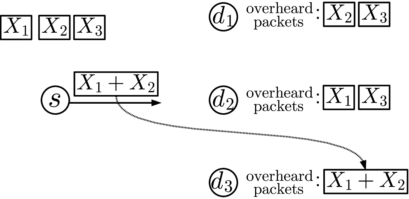
In Fig. 2(a), source $s$ would like to serve three receivers $d_{1}$ to $d_{3}$. Each $(s,d_{k})$ session contains a single information packet $X_{k}$, and the goal is to convey each $X_{k}$ to the intended receiver $d_{k}$ for all $k=1,2,3$. Suppose the 2-phase approach in Section II-C is used. During Phase 1, each packet is sent repeatedly until it is received by at least one receiver, which either conveys the packet to the intended receiver or creates an overheard packet that can be used in Phase 2. Suppose after Phase 1, $d_{1}$ has received $X_{2}$ and $X_{3}$, $d_{2}$ has received $X_{1}$ and $X_{3}$, and $d_{3}$ has not received any packet (Fig. 2(a)). Since each packet has reached at least one receiver, source $s$ moves to Phase 2.

One can easily check that if $s$ sends out a coded packet $[X_{1}+X_{2}]$ in Phase 2, such packet can serve both $d_{1}$ and $d_{2}$. That is, $d_{1}$ (resp. $d_{2}$) can decode $X_{1}$ (resp. $X_{2}$) by subtracting $X_{2}$ (resp. $X_{1}$) from $[X_{1}+X_{2}]$. Nonetheless, since the broadcast PEC is random, the coded packet $[X_{1}+X_{2}]$ may or may not reach $d_{1}$ or $d_{2}$. Suppose that due to random channel realization, $[X_{1}+X_{2}]$ reaches only $d_{3}$, see Fig. 2(a). The remaining question is what $s$ should send for the next time slot. For the following, we compare the existing 2-phase approach and a new optimal decision.

The existing 2-phase approach: We first note that since $d_{3}$ received neither $X_{1}$ nor $X_{2}$ in the past, the newly received $[X_{1}+X_{2}]$ cannot be used by $d_{3}$ to decode any information packet. In the existing results [15, 19, 9], $d_{3}$ thus discards the overheard $[X_{1}+X_{2}]$, and $s$ would continue sending $[X_{1}+X_{2}]$ for the next time slot in order to capitalize this coding opportunity created in Phase 1.

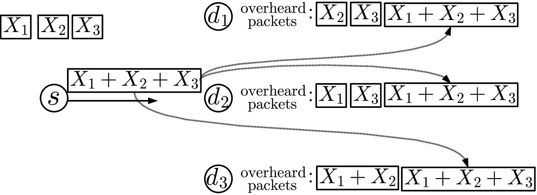
The optimal decision: It turns out that the broadcast system can actually benefit from the fact that $d_{3}$ overhears the coded packet $[X_{1}+X_{2}]$ even though neither $X_{1}$ nor $X_{2}$ can be decoded by $d_{3}$. More explicitly, instead of sending $[X_{1}+X_{2}]$, $s$ should send a new packet $[X_{1}+X_{2}+X_{3}]$ that mixes all three sessions together. With the new $[X_{1}+X_{2}+X_{3}]$ (see Fig. 2(b) for illustration), $d_{1}$ can decode the desired $X_{1}$ by subtracting both $X_{2}$ and $X_{3}$ from $[X_{1}+X_{2}+X_{3}]$. $d_{2}$ can decode the desired $X_{2}$ by subtracting both $X_{1}$ and $X_{3}$ from $[X_{1}+X_{2}+X_{3}]$. For $d_{3}$, even though $d_{3}$ does not know the values of $X_{1}$ and $X_{2}$, $d_{3}$ can still use the previously overheard $[X_{1}+X_{2}]$ packet to subtract the interference $(X_{1}+X_{2})$ from $[X_{1}+X_{2}+X_{3}]$ and decode its desired packet $X_{3}$. As a result, the new coded packet $[X_{1}+X_{2}+X_{3}]$ serves all destinations $d_{1}$, $d_{2}$, and $d_{3}$, simultaneously. This new coding decision thus strictly outperforms the existing 2-phase approach.

Two critical observations can be made for this example. First of all, when $d_{3}$ overhears a coded $[X_{1}+X_{2}]$ packet, even though $d_{3}$ can decode neither $X_{1}$ nor $X_{2}$, such new side information can still be used for future decoding. More explicitly, as long as $s$ sends packets that are of the form $\alpha(X_{1}+X_{2})+\beta X_{3}$, the “aligned interference” $\alpha(X_{1}+X_{2})$ can be completely removed by $d_{3}$ without decoding individual $X_{1}$ and $X_{2}$. This technique is thus termed “code alignment,” which is in parallel with the interference alignment method used in Gaussian interference channels [3]. Second of all, in the existing 2-phase approach, Phase 1 has the dual roles of sending uncoded packets to their intended receivers, and, at the same time, creating new coding opportunities (the overheard packets) for Phase 2. It turns out that this dual-purpose Phase-1 operation is indeed optimal (as will be seen in Sections IV and V). The suboptimality of the 2-phase approach for $K>2$ is actually caused by the Phase-2 operation, in which source $s$ only capitalizes the coding opportunities created in Phase 1 but does not create any new coding opportunities for subsequent packet mixing. One can thus envision that for the cases $K>2$, an optimal policy should be a multi-phase policy, say an $M$-phase policy, such that for all $i\in[M-1]$ (not only for the first phase) the packets sent in the $i$-th phase have dual roles of sending the information packets to their intended receivers and simultaneously creating new coding opportunities for the subsequent Phases $(i+1)$ to $M$. These two observations will be the building blocks of our achievability results.

We define any bijective function $\pi:[K]\mapsto[K]$ as a $K$-permutation and we sometimes just say that $\pi$ is a permutation whenever it is clear from the context that we are focusing on $[K]$. There are totally $K!$ distinct $K$-permutations. Given any $K$-permutation $\pi$, for all $j\in[K]$ we define $S^{\pi}_{j}\stackrel{{\scriptstyle\Delta}}{{=}}\{\pi(l):\forall l\in[j]\}$ as the set of the first $j$ elements according to the permutation $\pi$. We then have the following capacity outer bound for any 1-to-$K$ broadcast PEC with COF.

For any given permutation $\pi$, consider a new broadcast channel with $(K-1)$ artificially created information pipes connecting all the receivers $d_{1}$ to $d_{K}$. More explicitly, for all $j\in[K-1]$, create an auxiliary pipe from $d_{\pi(j)}$ to $d_{\pi(j+1)}$. See Fig. 3 for illustration. With the auxiliary pipes, any destination $d_{\pi(j)}$, $j\in[K]$, not only observes the corresponding output $Z_{\pi(j)}$ of the broadcast PEC but also has all the information $Z_{\pi(l)}$ of its “upstream receivers” $d_{\pi(l)}$ for all $l\in[j-1]$. Since we only create new pipes, any achievable rates of the original 1-to-$K$ broadcast PEC with COF must also be achievable in the new 1-to-$K$ broadcast PEC with COF in Fig. 3. The capacity of the new 1-to-$K$ broadcast PEC with COF is thus an outer bound on the capacity of the original 1-to-$K$ broadcast PEC with COF.

On the other hand, the new 1-to-$K$ broadcast PEC in Fig. 3 is a physically degraded broadcast channel with the new success probability of $d_{k}$ being $p_{\cup S_{k}^{\pi}}$ instead of $p_{\pi(k)}$ (see Fig. 3). [8] shows that COF does not increase the capacity of any physically degraded broadcast channel. Therefore the capacity of the new 1-to-$K$ broadcast PEC with COF is identical to the capacity of the new 1-to-$K$ broadcast PEC without COF. Since (3) is the capacity of the new 1-to-$K$ broadcast PEC without COF, (3) must be an outer bound of the capacity of the original 1-to-$K$ PEC with COF. By considering different permutation $\pi$, the proof of Proposition 1 is complete.  ∎

For the following, we first provide the capacity results for general 1-to-3 broadcast PECs. We then state an achievability inner bound for general 1-to-$K$ broadcast PECs with COF for arbitrary $K$ values, which, together with the outer bound in Proposition 1 can effectively bracket the capacities for the cases in which $K\geq 4$.

To state the capacity inner bound, we need to define an additional function: $f_{p}(S\overline{T})$, which takes an input $S\overline{T}$ of two disjoint sets $S,T\in 2^{[K]}$. More explicitly, we define $f_{p}(S\overline{T})$ as the probability that a packet $Y$, transmitted through the 1-to-$K$ PEC, is received by all those $d_{i}$ with $i\in S$ and not received by any $d_{j}$ with $j\in T$. For example, $f_{p}(S\overline{[K]\backslash S})=p_{S\overline{[K]\backslash S}}$ for all $S\in 2^{[K]}$. For arbitrary disjoint $S$ and $T$, we thus have

We also say that a strict total ordering “$\prec$” on $2^{[K]}$ is cardinality-compatible if

For example, for $K=3$, the following strict total ordering

is cardinality-compatible.

Since Proposition 3 holds for any cardinality-compatible, strict total ordering $\prec$. We can easily derive the following corollary:

To distinguish different strict total orderings, we append a subscript $l$ to $\prec$. For example, $\prec_{1}$ and $\prec_{2}$ correspond to two distinct strict total orderings. Overall, there are $L\stackrel{{\scriptstyle\Delta}}{{=}}\prod_{k=0}^{K}\left({K\choose k}!\right)$ distinct strict total ordering $\prec_{l}$, $\forall l\in[L]$, that are cardinality-compatible.

Remark: For some general classes of PEC parameters, one can prove that the inner bound of Proposition 3 is indeed the capacity region for arbitrary $K\geq 4$ values. Two such classes are discussed in the next subsection.

We first provide the capacity results for symmetric broadcast PECs.

The perfect channel symmetry condition in Proposition 4 may be a bit restrictive for real environments as most broadcast channels are non-symmetric. A more realistic setting is to allow channel asymmetry while assuming spatial independence between different destinations $d_{i}$.

Note: A symmetric 1-to-$K$ broadcast PEC needs not be spatially independent. A spatially independent PEC is symmetric if $p_{1}=p_{2}=\cdots=p_{K}$.

To describe the capacity results for spatially independent 1-to-$K$ PECs, we need the following additional definition.

The one-sided fairness contains many practical scenarios of interest. For example, the perfectly fair rate vector $(R,R,\cdots,R)$ by definition is also one-sidedly fair. Another example is when $\min(p_{1},\cdots,p_{K})>\frac{1}{2}$ and we allow the rate $R_{k}$ to be proportional to the corresponding marginal success probability $p_{k}$, i.e., $R_{k}=p_{k}R$, then the rate vector $(p_{1}R,p_{2}R,\cdots,p_{K}R)$ is also one-sidedly fair.

For the following, we provide the capacity of spatially independent 1-to-$K$ PECs with COF under the condition of one-sided fairness.

Proposition 5 implies that Proposition 1 is indeed the capacity region when focusing on the one-sidedly fair rate region $\Lambda_{\text{osf}}$.

The packet evolution scheme is described as follows. Recall that each $(s,d_{k})$ session has $nR_{k}$ information packets $X_{k,1}$ to $X_{k,nR_{k}}$. We associate each of the $\sum_{k=1}^{K}nR_{k}$ information packets with an intersession coding vector ${\mathbf{v}}$ and a set $S\subseteq[K]$. An intersession coding vector is a $\left(\sum_{k=1}^{K}nR_{k}\right)$-dimensional row vector with each coordinate being a scalar in $\mathop{\sf GF}\limits(q)$. Before the start of the broadcast, for any $k\in[K]$ and $j\in[nR_{k}]$ we initialize the corresponding vector ${\mathbf{v}}$ of $X_{k,j}$ in a way that the only nonzero coordinate of ${\mathbf{v}}$ is the coordinate corresponding to $X_{k,j}$ and all other coordinates are zero. Without loss of generality, we set the value of the only non-zero coordinate to one. That is, initially the coding vectors ${\mathbf{v}}$ are set to the elementary basis vectors of the entire $\left(\sum_{k=1}^{K}nR_{k}\right)$-dimensional message space.

For any $k\in[K]$ and $j\in[nR_{k}]$ the set $S$ of $X_{k,j}$ is initialized to $\emptyset$. As will be clear shortly after, we call $S$ the overhearing set³³ 3 Unlike the existing results [11], in this work the overhearing set does not mean that the receivers $d_{i}$ in $S(X_{k,j})$ have known the value of $X_{k,j}$. Detailed discussion of the overhearing set $S(X_{k,j})$ are provided in Lemma 2. of the packet $X_{k,j}$. For easier reference, we use ${\mathbf{v}}(X_{k,j})$ and $S(X_{k,j})$ to denote the intersession coding vector and the overhearing set of $X_{k,j}$.

Throughout the $n$ broadcast time slots, source $s$ constantly updates the $S(X_{k,j})$ and ${\mathbf{v}}(X_{k,j})$ according to the COF. The main structure of a packet evolution scheme can now be described as follows.

In summary, a group of target packets $\{X_{k,j_{k}}\}$ are selected according to the choice of the subset $T$. The corresponding vectors $\{{\mathbf{v}}(X_{k,j_{k}})\}$ are used to construct a coding vector ${\mathbf{v}}_{\text{tx}}$. The same coded packet $Y_{\text{tx}}$, corresponding to ${\mathbf{v}}_{\text{tx}}$, is then sent repeatedly for many time slots until one of the target packets $X_{k,j_{k}}$ evolves (when the corresponding $S(X_{k,j_{k}})$ changes). Then a new subset $T$ is chosen and the process is repeated until we use up all $n$ time slots. Three subroutines are used as the building blocks of a packet evolution method: (i) How to choose the non-empty $T\subseteq[K]$; (ii) For each $k\in[K]$, how to select a single target packets $X_{k,j_{k}}$ among all $X_{k,j}$ satisfying $(S(X_{k,j})\cup\{k\})\supseteq T$; and (iii) How to update the coding vectors ${\mathbf{v}}(X_{k,j_{k}})$ and the overhearing sets $S(X_{k,j_{k}})$. For the following, we first describe the detailed update rules.

Let us revisit the optimal coding scheme of the example in Fig. 2 of Section II-D. Before broadcast, the three information packets $X_{1}$ to $X_{3}$ have the corresponding ${\mathbf{v}}$ and $S$: ${\mathbf{v}}(X_{1})=(1,0,0)$, ${\mathbf{v}}(X_{2})=(0,1,0)$, and ${\mathbf{v}}(X_{3})=(0,0,1)$, and $S(X_{1})=S(X_{2})=S(X_{3})=\emptyset$. We use the following table for summary.

Consider a duration of 5 time slots.

Slot 1: Suppose that $s$ chooses $T=\{1\}$. Since $(\emptyset\cup\{1\})\supseteq T$, Packet Selection outputs $X_{1}$. The coding vector ${\mathbf{v}}_{\text{tx}}$ is thus a scaled version of ${\mathbf{v}}(X_{1})=(1,0,0)$. Without loss of generality, we choose ${\mathbf{v}}_{\text{tx}}=(1,0,0)$. Based on ${\mathbf{v}}_{\text{tx}}$, $s$ transmits a packet $1X_{1}+0X_{2}+0X_{3}=X_{1}$. Suppose $[X_{1}]$ is received by $d_{2}$, i.e., $S_{\text{rx}}=\{2\}$. Then during Update, $S_{\text{rx}}=\{2\}\nsubseteq S(X_{1})=\emptyset$. Update thus sets $S(X_{1})=\{2\}$ and ${\mathbf{v}}(X_{1})={\mathbf{v}}_{\text{tx}}=(1,0,0)$. The packet summary becomes

Slot 2: Suppose that $s$ chooses $T=\{2\}$. Since $(\emptyset\cup\{2\})\supseteq T$, Packet Selection outputs $X_{2}$. The coding vector ${\mathbf{v}}_{\text{tx}}$ is thus a scaled version of ${\mathbf{v}}(X_{2})=(0,1,0)$. Without loss of generality, we choose ${\mathbf{v}}_{\text{tx}}=(0,1,0)$ and accordingly $[X_{2}]$ is sent. Suppose $[X_{2}]$ is received by $d_{1}$, i.e., $S_{\text{rx}}=\{1\}$. Since $S_{\text{rx}}\nsubseteq S(X_{2})$, after Update the packet summary becomes

Slot 3: Suppose that $s$ chooses $T=\{3\}$ and Packet Selection outputs $X_{3}$. The coding vector ${\mathbf{v}}_{\text{tx}}$ is thus a scaled version of ${\mathbf{v}}(X_{3})=(0,0,1)$, and we choose ${\mathbf{v}}_{\text{tx}}=(0,0,1)$. Accordingly $[X_{3}]$ is sent. Suppose $[X_{3}]$ is received by $d_{1}$ and $d_{2}$, i.e., $S_{\text{rx}}=\{1,2\}$. Then after Update, the packet summary becomes

Slot 4: Suppose that $s$ chooses $T=\{1,2\}$. Since $(S(X_{1})\cup\{1\})\supseteq T$ and $(S(X_{2})\cup\{2\})\supseteq T$, Packet Selection outputs $\{X_{1},X_{2}\}$. ${\mathbf{v}}_{\text{tx}}$ is thus a linear combination of ${\mathbf{v}}(X_{1})=(1,0,0)$ and ${\mathbf{v}}(X_{2})=(0,1,0)$. Without loss of generality, we choose ${\mathbf{v}}_{\text{tx}}=(1,1,0)$ and accordingly $[X_{1}+X_{2}]$ is sent. Suppose $[X_{1}+X_{2}]$ is received by $d_{3}$, i.e., $S_{\text{rx}}=\{3\}$. Then during Update, for $X_{1}$, $S_{\text{rx}}=\{3\}\nsubseteq S(X_{1})=\{2\}$. Update thus sets $S(X_{1})=\{2,3\}$ and ${\mathbf{v}}(X_{1})={\mathbf{v}}_{\text{tx}}=(1,1,0)$. For $X_{2}$, $S_{\text{rx}}=\{3\}\nsubseteq S(X_{2})=\{1\}$. Update thus sets $S(X_{2})=\{1,3\}$ and ${\mathbf{v}}(X_{2})={\mathbf{v}}_{\text{tx}}=(1,1,0)$. The packet summary becomes

References

- [1] S. Avestimehr, S. Diggavi, and D. Tse, “A deterministic approach to wireless relay network,” in Proc. 45th Annual Allerton Conf. on Comm., Contr., and Computing. Monticello, IL, September 2007.
- [2] P. Bergmans, “Random coding theorem for broadcast channels with degraded components,” IEEE Trans. Inform. Theory, vol. 19, pp. 197–207, March 1973.
- [3] V. Cadambe and S. Jafar, “Interference alignment and degrees of freedom of the -user interference channel,” IEEE Trans. Inform. Theory, vol. 54, no. 8, pp. 3425–3441, August 2008.
- [4] P. Chou, Y. Wu, and K. Jain, “Practical network coding,” in Proc. 41st Annual Allerton Conf. on Comm., Contr., and Computing. Monticello, IL, October 2003.
- [5] T. M. Cover, “Comments on broadcast channels,” IEEE Trans. Inform. Theory, vol. 44, no. 6, pp. 2524–2530, Oct. 1998.
- [6] A. Dana, R. Gowaikar, R. Palanki, B. Hassibi, and M. Effros, “Capacity of wireless erasure networks,” IEEE Trans. Inform. Theory, vol. 52, no. 3, pp. 789–804, March 2006.
- [7] A. Das, S. Vishwanath, S. Jafar, and A. Markopoulou, “Network coding for multiple unicasts: An interference alignment approach,” in Proc. IEEE Int’l Symp. Inform. Theory. Austin, Texas, USA, June 2010.
- [8] A. El Gamal, “The feedback capacity of degraded broadcast channels,” IEEE Trans. Inform. Theory, vol. 25, no. 2, pp. 379–381, March 1978.
- [9] L. Georgiadis and L. Tassiulas, “Broadcast erasure channel with feedback — capacity and algorithms,” in Proc. 5th Workshop on Network Coding, Theory, & Applications (NetCod). Lausanne, Switzerland, June 2009, pp. 54–61.
- [10] T. Ho, M. Médard, R. Koetter, D. Karger, M. Effros, J. Shi, and B. Leong, “A random linear network coding approach to multicast,” IEEE Trans. Inform. Theory, vol. 52, no. 10, pp. 4413–4430, October 2006.
- [11] S. Katti, H. Rahul, W. Hu, D. Katabi, M. Médard, and J. Crowcroft, “XORs in the air: Practical wireless network,” in Proc. ACM Special Interest Group on Data Commun. (SIGCOMM), 2006.
- [12] J. Körner and K. Marton, “General broadcast channels with degraded message sets,” IEEE Trans. Inform. Theory, vol. 23, no. 1, pp. 60–64, January 1977.
- [13] D. Koutsonikolas, C.-C. Wang, and Y. Hu, “CCACK: Efficient network coding based opportunistic routing through cumulative coded acknowledgments,” in Proc. 29th IEEE Conference on Computer Communications (INFOCOM). San Diego, USA, March 2010, pp. 1–9.
- [14] ——, “ECR: enhanced coded retransmission for downlink access-point networks,” in ACM CoNEXT, 2010, to be submitted.
- [15] P. Larsson and N. Johansson, “Multi-user ARQ,” in Proc. IEEE Vehicular Technology Conference, 2006.
- [16] S.-Y. Li, R. Yeung, and N. Cai, “Linear network coding,” IEEE Trans. Inform. Theory, vol. 49, no. 2, pp. 371–381, February 2003.
- [17] X. Li, C.-C. Wang, and X. Lin, “Throughput and delay analysis on uncoded and coded wireless broadcast with hard deadline constraints,” in Proc. 29th IEEE Conference on Computer Communications (INFOCOM). San Diego, USA, March 2010, pp. 1–5.
- [18] L. Ozarow and S. Leung-Yan-Cheong, “An achievable region and outer bound for the Gaussian broadcast channel with feedback,” IEEE Trans. Inform. Theory, vol. 30, no. 4, July 1984.
- [19] E. Rozner, A. Iyer, Y. Mehta, L. Qiu, and M. Jafry, “ER: Efficient retranmission scheme for wireless LANs,” in Proc. ACM CoNEXT. New York, USA, December 2007.
- [20] J. Sundararajan, D. Shah, and M. Médard, “ARQ for network coding,” in Proc. IEEE Int’l Symp. Inform. Theory. Toronto, Canada, July 2008.
- [21] C.-C. Wang, “On the capacity of wireless 1-hop intersession network coding — a broadcast packet erasure channel approach,” in Proc. IEEE Int’l Symp. Inform. Theory. Austin, TX, USA, June 2010.
- [22] C.-C. Wang, A. Khreishah, and N. Shroff, “Cross-layer optimizations for intersession network coding on practical 2-hop relay networks,” in Proc. 43rd Asilomar Conference on Signals, Systems and Computers. Pacific Grove, CA, USA, November 2009, pp. 771–775.
- [23] H. Weingarten, Y. Steinberg, and S. Shamai, “The capacity region of the Gaussian multiple-input multiple-output broadcast channel,” IEEE Trans. Inform. Theory, vol. 52, no. 9, pp. 3936–3964, September 2006.
- [24] Y. Wu, “Broadcasting when receivers know some messages a priori,” in Proc. IEEE Int’l Symp. Inform. Theory. Nice, France, June 2007, pp. 1141–1145.
- [25] F. Xue and X. Yang, “Network coding and packet-erasure broadcast channel,” in Proc. the 5th IEEE Annual Communications Society Conference on Sensor, Mesh and Ad Hoc Communications and Networks Workshops (SECON). San Francisco, CA, USA, July 2008.