Anomalous decays of pseudoscalar mesons
von
Thimo Petri
Diplomarbeit in Physik
angefertigt am
Institut für Kernphysik
Forschungszentrum Jülich
vorgelegt der
Mathematisch-Naturwissenschaftlichen Fakultät
der
Rheinischen Friedrich-Wilhelms-Universität Bonn
im Juli/2010
Ich versichere, dass ich diese Arbeit selbständig verfasst und keine anderen als die angegebenen Quellen und Hilfsmittel benutzt sowie die Zitate kenntlich gemacht habe.
| Referent: | PD Dr. Andreas Wirzba |
| Koreferent: | Prof. Dr. Ulf-G. Meißner |
Chapter 1 Introduction
In this work we will discuss decays of the pseudoscalar mesons (, and ) which are governed by the chiral anomaly. The chiral anomaly is the non conservation of the axial vector current under quantization when gauge fields are present.
The anomalous decays of the were first measured in the 1960s ([1, 2]and [3]) and have been updated in the recent years [4]. Moreover, many calculations were performed in this sector, see e.g. [5, 6, 7, 8] and [9]. Some of these decays are of special interest because their study permits a deep insight into aspects of modern physics. Through the decays and the single or double off-shell behavior, respectively, of the pion-2-photon vertex can be analyzed. The decay was first measured by [10, 11]. Even most recent calculations ([12, 13, 14]) are still three standard deviations away from the modern measurements ([15]). This may open a window for the search of new physics.
By recent measurements of so-called -factories, e.g. WASA@CELSIUS, WASA@COSY ([16]), CB@MAMI, KLOE@DANE ([17]) or the CMD-2 Collaboration ([18]), the decays of the meson have become an important subject of modern hadron physics. Analogous to the -decays, the theoretical calculations of the decays , and can now be tested by modern measurements. While all the above mentioned decays proceed via the triangle anomaly, a study of the box anomaly is possible as well. This can be done by analyzing the decays and , see e.g. [19, 20] and [21, 22], respectively. Particularly these decays admit a study of CP-violations beyond the standard model. The decay allows a test of a formally unchecked CP-violating formalism. In the decay CP-violation can be observed via asymmetry measurements of the - with respect to the decay planes. Theoretical discussions can be found in [23], while measurements were done recently by KLOE@DANE ([17]) and are in progress by WASA@COSY.
In the sector experimental data are very scarce and only few theoretical calculations were done. New measurements are in progress, but it will take some time until precise findings can be expected. Still, theoretical predictions can be made. In addition to the analogous decays of the -sector, also the decay is kinematically allowed. Since the aim of this work is the study of the anomalous -decays and analogous decays in the - and -sector, -decays as the above mentioned process will not be discussed here.
Extrapolated to the chiral point, all anomalous decays are solely determined by the Wess-Zumino-Witten Lagrangian ([24, 25]). As we will see for decays into off-shell photon(s), we have to take the momentum dependency of the form factors into account. To describe that we will apply vector meson dominance (VMD) models. Over the years the so called hidden gauge model ([26, 27, 28]) has reached good agreement with the experimental data. Modern refinements were introduced by the authors of [29, 30] and [31] in the last years. We will calculate the decay rates and branching ratios for all mentioned decays using the hidden gauge model and its modern update in order to discuss the ability of these models to describe the experimental data.
This work is organized as follows. In the second Chapter we will give a short overview over pseudoscalar mesons and their decay channels. We will discuss symmetries in general in order to analyze the axial anomaly in particular. Thereafter we derive the Wess-Zumino-Witten Lagrangian according to [24, 25] and present the contact terms which determine the chiral triangle and box anomaly at the chiral point. The concept of vector mesons as dynamical gauge bosons of hidden local symmetries will be discussed to explain the solutions of the anomaly equation in the presence of vector mesons. Thereby we can present the mentioned vector meson dominance models (the hidden gauge model and the modified vector meson dominance model [29, 30] and [31]) which will be used in the following chapters.
The third Chapter contains the derivations of the decay rates and branching ratios of all mentioned anomalous decays. We will differentiate between the decays proceeding via the triangle anomaly and the ones progressing via the box anomaly, because each sector is separately governed by closely related form factors. We also present extensive discussions of the vector meson form factors for each decay. In the case of the box-anomaly decays, we will emphasize the contributions of the CP-violating form factors in addition to the leading-order contribution.
The calculations are presented in detail to be comprehensible for future students. Up to Chapter 3, this work can be seen as a handbook for anomalous decays, which is actually the reason for the detailed presentation of the calculations.
In the fourth Chapter we will discuss the results calculated for the decay rates and branching ratios with the various vector meson dominance models. We will show the dependence of the decay rates on the invariant masses of the outgoing particles and compare our results for the branching ratios to other theoretical works and experimental data.
In the last Chapter we give a conclusion of our work and a brief outlook on further studies.
Chapter 2 Theoretical background
2.1 Pseudoscalar mesons
In the quark model the different hadrons are classified according to their quark content. Because these particles are color-neutral states, hadrons have to be constructed from a quark and an antiquark or three valence quarks (or antiquarks). The hadrons constructed by two valence quarks , a quark and an anti-quark with color and ’anti-color’, respectively, are called mesons. The hadrons with three quarks with suitable colors are called baryons. These valence quarks give rise to the quantum numbers of the hadrons via their flavor and via their symmetry . Here is the total angular momentum containing orbital angular momentum and spin , while and stands for parity and charge conjugation. Baryons are constructed from three quarks, respectively, three antiquarks. Thus they are fermions. Mesons contain a quark-antiquark pair and thus are bosons. In the following work we are only interested in light mesons built by up, down or strange quarks, which are subject to an approximate U(3) flavor symmetry. The resulting nine states can be decomposed into a singlet and an octet state. Written in group notation this means:
| (2.1) |
The different mesons can be classified into types according to their spin configurations.
| Type | |||||
| Pseudoscalar meson | 0 | 0 | - | 0 | |
| Axial vector meson | 0 | 1 | + | 1 | |
| Vector meson | 1 | 0 | - | 1 | |
| Scalar meson | 1 | 1 | + | 0 | |
| Tensor meson | 1 | 1 | + | 2 | |
| … | |||||


The different types are shown in Table 2.1. The nonet of the pseudoscalar mesons () and the nonet of the vector mesons are shown in Figure 2.2 and Figure 2.2. Here the charge increases towards the right and the strangeness increases towards the upward direction. Note, that and are not the exact octet and singlet states, respectively. These are denoted by and . The physical, measured particles are mixings between the and states with an --mixing angle [32]. These states can be constructed from the flavor states according to
| (2.2) |
Since we want to study the decay of the pseudoscalar mesons and , we first give some general informations of this particles and then show their different decay modes.
The is the lightest meson with a mass of [33]. The quark content is:
| (2.3) |
Like all mesons, the pion is unstable, however w.r.t. electroweak decays. The decay modes are given in Table 2.2.
| Mode | Branching ratio |
|---|---|
| positronium | |
The and - in comparison to the pion - have also strange quark content:
| (2.4) | |||||
| (2.5) |
The masses of the mesons are and . The total decay widths were measured to for the -meson and for the . The decay modes and branching ratios are given in Table 2.3 and Table 2.4.
| Mode | Branching ratio |
|---|---|
| invisible | |
| Mode | Branching ratio |
|---|---|
| (including non-resonant ) | |
| neutrals | |
2.2 Symmetries and anomalies
Transformations which do not change the physics of a system are symmetry
transformations. In classical physics this means that the
action and thereby the equation of motion are unchanged. In a quantum mechanical
formulation, e.g. in a path integral formalism, a symmetry is given if the
Lagrangian and the path integral measure are invariant under the respective
transformation. The relationship between symmetries and conversation laws is
expressed via the Noether theorem which says that for every continuous
transformation that leaves the action invariant there exists a time
independent classical charge and a corresponding conserved current
.
There exist many different kinds of symmetries, which are all
realized by nature. We give a short overview and examples:
- •
exact symmetry: examples for exact symmetries are the electromagnetic gauge or the color symmetry of QCD;
- •
anomalous symmetry: If a classical symmetry is broken in quantum physics it is called anomalous. It is not a true symmetry. An example is the axial symmetry, which will be discussed below;
- •
explicitly broken symmetry: the symmetry is explicitly broken by a term in the Lagrangian that does not preserve the invariance. If this term is very small it is an approximate symmetry. The isospin symmetry is a common example;
- •
hidden symmetry: if the Lagrangian is invariant, but not the ground state the symmetry is called hidden. Examples are the broken invariance by Higgs fields (spontaneous symmetry breaking) or the chiral symmetry in the strong interactions (dynamical symmetry breaking).
We are interested in the chiral axial anomaly. The concept of anomalies was introduced by Adler, Bell and Jackiw ([35, 36]) and also by Fujikawa [37] via path integral formalism. We will give a short
overview of the calculations given in Chapter 19 of
[38].
In the massless Dirac
Lagrangian the left- and right- handed
fermions are decoupled and the Lagrangian is therefore invariant under the transformation of the fields11
1
We use the standard notation of the -matrices according to [39]. The parameter is real valued and is the total antisymmetric tensor in 3+1 dimensions:
| (2.6) |
The corresponding axial current
| (2.7) |
is classically conserved,
| (2.8) |
This does not hold quantum mechanically when gauge fields are present. The axial vector
current is built from two fermion fields. Because
the product of two local operators can induce singularities, we separate their
locations and , and take the limit in the
end. This is visualized in Figure 2.3.
The lowest order contribution (without background gauge fields) results in zero, because we have to take the trace over three -matrices. The next
order contribution instead gives a nonvanishing result. Therefore the
divergence of the current has the following form,
| (2.9) |
which is known as Adler-Bell-Jackiw anomaly [35, 36]. is the electromagnetic field strength tensor, .

Another approach uses the path integral method. The result is that the conservation of the axial current clashes with the gauge invariance of the fields. The transformation of the functional measure of the path integral gives an additional contribution via the Jacobian
| (2.10) |
In this case the divergence of the axial vector current reads as
| (2.11) |
where with d the number of space time dimensions. Taking reproduces exactly the Adler-Bell-Jackiw anomaly given in (2.9). The discussion in QCD is quite similar. The transformation has the following form
| (2.12) |
where with the Gell-Mann Matrix . The corresponding axial current reads:
| (2.13) |
The calculations done for the QED sector are valid here as well, either in the point splitting formalism via radiative corrections or in the path integral formalizm due to the jacobian. This yields the following result
| (2.14) |
with the gluon field strength tensor and the color matrices . Because of the flavor trace this term actually vanishes. We see that the axial flavor currents have no anomaly in QCD. But there is an anomaly in the electromagnetic sector which is given by
| (2.15) |
Here is the matrix of the electric charges of the quarks,
| (2.16) |
Since
| (2.17) |
Note, that annihilates a and we therefore get the anomaly contribution to the decay .
2.3 Wess-Zumino-Witten Lagrangian (WZW)
We want to present briefly the effective Wess-Zumino-Witten Lagrangian, which
summarizes and determines the effects of anomalies in current algebra. The
discussion will follow the presentation of [24] and [25].
The QCD Lagrangian is given by:
| (2.18) |
with
| (2.19) |
where is the vector field of the gluons, is the field strength tensor. Because of the inherent nonlinearity and the large effective coupling constant in the non-perturbative regime, it is difficult to derive predictions about hadrons directly from the QCD Lagrangian. The most successful way to deal with it is lattice QCD, although it needs very large computational power and the theoretical insight is limited. In the low-energy sector chiral perturbation theory (PT) as low-energy effective field theory of QCD has been successfully applied. Low energy PT exploits the global symmetry of the QCD Lagrangian in the limit of vanishing quark masses, which was mentioned in the previous Section. The lowest order effective chiral action is given by:
| (2.20) |
with the chiral unitary matrix
| (2.21) |
and is the physical pion decay constant and are the pseudoscalar fields
| (2.22) |
This Lagrangian does not only contain all symmetries of the QCD Lagrangian, but possesses
extra symmetries, which are not present in the QCD Lagrangian. According to
[25] these symmetries are naive parity
conjugation and a symmetry which counts the number of the
Goldstone bosons modulo two. These separately are not symmetries of the QCD Lagrangian,
but form a symmetry (total parity) if they are combined.
The equation of motion derived from (2.20) in the case without external fields is given by:
| (2.23) |
As shown in [25], the equation of motion which violates naive parity can be constructed by adding a symmetry violating extra term with the smallest possible number of derivatives. This is given by
| (2.24) |
Here is a constant. Note, that typically there appears a four-dimensional antisymmetric tensor due to the violation of the naive parity conjugation.
The next step is to construct a higher order Lagrangian which leads to this
equation of motion. The derivation is quite complicated and can be found
in [25].
Because it is not possible to construct a closed form expression in four dimensions which breaks the symmetries the Wess Zumino action is constructed in five dimensions [25]:
| (2.25) |
This integral over a five-dimensional Manifold can be expressed by Stokes’ theorem as an integral over the boundary of , which is ordinary Minkowski space .
This action is invariant under global charge rotations , where is a constant and the electric charge matrix of quarks. By turning this into a local symmetry also the Wess-Zumino action changes to:
| (2.26) | |||||
and the effective Lagrangian becomes:
| (2.27) |
which can be found in many publications, e.g
[40, 41, 42, 43] and also
in [32].
Note that after expanding and integrating by parts one can find
| (2.28) |
with the number of colors, which is exactly the part that describes the decay . The author of ref [25] also found that the Noether coupling describes a -vertex:
| (2.29) |
This vertex describes the coupling of a photon to three pseudoscalar mesons
and therefore the decays .
In summary the
Wess-Zumino-Witten Lagrangian already determines the triangle anomaly sector
via and the box anomaly sector via .
2.4 Vector meson dominance (VMD)
Using the WZW Lagrangian the decay of a pseudoscalar particle into two photons is described very well, as we will see in the next Chapter. Because the theoretical predictions for other anomalous decays differ from the experimental data an extended model is needed. Vector meson dominance models have reached good agreement in describing the experimental data of the triangle anomaly sector and are also valid in the box anomaly sector.
Original work for the so-called hidden gauge model has been done by [26, 44]. Overviews can be
found in [45] and [46]. We will present this subject according to [27]
and discuss the so-called ’total vector meson dominance’, the ’hidden gauge model’ and modern
improvements done by [29, 30] and [31] afterwards.
Vector mesons as dynamical gauge bosons of hidden local symmetries and the low-energy theorem
The nonlinear sigma model based on the manifold is a low energy effective theory of massless 3-flavored
QCD. The global symmetry is spontaneously broken down to the diagonal subgroup
. The dynamical gauge bosons of the hidden local symmetry
can be modelled as the vector mesons (). In this framework the KSFR relation and the
universally of -coupling can be shown (see [47, 48]).
Following [27] we introduce the variables and as
| (2.30) |
and non-abelian gauge fields . The global group is gauged with external fields and such that the corresponding covariant derivatives are given as
| (2.31) |
In the following we simplify
| (2.32) |
where is the electromagnetic field.
Using this, the Lagrangian reads
| (2.33) |
with an arbitrary parameter . In this term stands for the kinetic terms of the gauge fields and
By fixing the hidden local gauge to , the Lagrangians, when expanded, yield the following relations:
| (2.34) | |||||
| (2.35) | |||||
| (2.36) |
When the parameter is eliminated from the first two relations the low-energy theorem of hidden local symmetry follows,
| (2.37) |
which is known as KSFR relation ([27]). By setting the parameter we get another KSFR relation namely and the universality of the vector meson coupling . This was postulated by Sakurai in 1960 [49].
Solutions to the anomaly equation in the presence of vector mesons
In the presence of vector mesons the anomaly equation has the form [27]
| (2.38) |
with a constants . Here the gauge variation contains also a hidden local symmetry transformation, such that . The anomaly equation is an inhomogeneous linear differential equation. So the solution will be a special solution of the inhomogeneous equation, for which we take the Wess-Zumino action (2.26), and general solutions of the homogenous equation. As shown in [27, 45] and [30] six invariants that conserve total parity but violate intrinsic parity can be found. According to [50, 51] and [52] two of these invariants are charge conjugation odd and can therefore be omitted. So the interesting part of the action is given by the Wess-Zumino action and the remaining four invariants,
| (2.39) |
These additional terms do not contribute to anomalous processes like in the chiral limit, but can contribute away from the chiral limit via vector mesons decaying into photons, since they have the same quantum numbers. So the anomalous Lagrangian including all couplings is given by [30]:
| (2.40) |
Here , and denote the vector meson, pseudoscalar and electromagnetic fields. The different Lagrangian pieces are given by
| (2.41) |
Here is the universal vector coupling constant, is the quark charge matrix given in (2.32) and is the number of colors. The pseudoscalar fields are defined as
| (2.42) |
and the vector meson fields read
| (2.43) |
Note that the prefactors of [30] based on the normalizations of [29] differ from ours.
The original terms of the WZW Lagrangian are of course the ones in (2.41) and
without vector
meson couplings. The first three Lagrangians contribute to the triangle
anomaly, while the last two contribute to the box anomaly sector.
The various vector meson dominance models
As one can see, the Lagrangians only depend on three different parameter
combinations, namely , and . These parameters have to be
fixed by comparison with data. For different choices of these parameter sets different vector meson dominance models result.
Before we present the different models, we can give some general conditions on
the parameters by discussing briefly the triangle sector. In Ref
[30] the amplitude for the decay
is derived from the Lagrangians given in (2.41):
| (2.44) |
To make sure that the vector meson dominance factor is normalized to one at and
to recover the original WZW term we
set . In this case the second Lagrangian will always vanish. We now
present the different VMD models.
The first one is the ’full vector meson dominance’:
| (2.45) |
Inserting these values of the parameters in (2.41), one can easily see that
the second, third and last Lagrangian, which are the ones involving photon
fields, vanish and so photons can only couple to pseudoscalar mesons via a
vector meson. Although this model is successfully describing data in the triangle
sector we will not deal with it in our work for the following reasons: (i) In the
box anomaly sector at the chiral point, full VMD does not
produce the WZW interaction. As pointed out in
[32], the full VMD model gives a 50% larger value
at zero four momentum than the anomaly. (ii) The authors of
[27] and [46] calculated that the decay rate
of the decay is times smaller than
the respective experimental data.
The following model, which we present, has the same predictions as the full VMD
model in the triangle sector, because the values of and are the
same, but it also agrees reasonably well with the accepted data referring to the
box anomaly as was shown in [32]. The parameters are in this case:
| (2.46) |
Here only the first and last Lagrangian in (2.41) give contributions,
while the others vanish. We will refer to this model as the hidden gauge model
(see e.g. [27]).
The next model, modified VMD, which is of interest, is a further extention of the hidden gauge
model. The authors of Refs. [29, 30] and [31]
fitted the c-parameters of the different Lagrangians and the coupling constant
to the data of the the processes
below a CM energy of 1.05 GeV. Note that the fitted processes do not include , so it will be of special
interest and a nice proof of the extended model to compare the results for
the different models in the sector.
Ref. [30] presented various fits, where different data sets have been taken into
account. Two of these fits were indicated as the ones that represent the data
the best. These fits are given in table 3 of [30] and were denoted by the conditions (i) Global Fit with ND+CMD and (ii) Global Fit
with ND+CMD++CMD2. The corresponding values for and are listed in Table 2.5.
| (i) | (ii) | |
|---|---|---|
Because the fits indeed give very similar values in our calculations we
will refer to them as one model and state the discrepancies as an error range.
The vector meson mass is related to the coupling constant and the parameter via
(2.36). Therefore there appear different vector meson masses in [30] which vary between
and in some of the fits. This will
contribute to the error of the results in the end.
2.5 Definitions
2.5.1 The decay momenta
In the next Chapter we will discuss the kinematics of the different decays of
the pseudoscalar mesons. Therefore we try to make common definition for the
four-momenta. This will work for every decay mode except the one into four
leptons, which we will relabel in the corresponding Chapter. The general
definitions are discussed here. Some further relations as well as a
comparison to the essential kinematics can be found in Appendix A.
The decay momenta of a pseudoscalar meson into two, three or four
particles are defined as follows:
such that the following relations for the four-momenta are valid in any frame:
Furthermore, we use the following notations: a four-momentum is denoted by an italic letter, e.g. , whereas the corresponding three-momentum is signalled by a bold-faced letter , i.e.
| (2.47) |
Moreover,
| (2.48) | |||||
| (2.49) | |||||
| (2.50) |
where is the momentum in the -direction.
2.5.2 The identification of the momenta
By comparing with the text below the cross section formula (38.19) of Ref. [34], the following identifications can easily be made:
| (2.51) | |||||
i.e., is the three-momentum of particle 1 in the rest frame of particle 1 and 2. Note that in analogy to Eq. (2.51)
| (2.52) |
Furthermore,
| (2.53) | |||||
| (2.54) | |||||
where
| (2.55) |
Thus, is the momentum of particle 3 in the rest frame of the decaying particle. Note that Eq. (2.55) allows to relate moduli of momenta in different frames:
| (2.56) |
The variables , and are invariant in all frames. We will give our results in terms of these standard variables.
2.5.3 The identification of the angles
Let us define the angle as the angle between the three-momentum and the direction in the rest frame:
| (2.57) |
Furthermore, we define the angle as the angle between the three-momentum and the direction in the rest frame:
| (2.58) |
is actullay the angle we will use in our discussions, so we will refer to as to make things easier. In analogy we can define as the angle between the three-momentum and the three-momentum in the rest frame. Note that the three-momentum in the rest frame points into the negative -direction
| (2.59) |
We also define , the azimuthal angle between the plane formed by in the rest frame and the corresponding plane formed by .
Chapter 3 Anomalous decays
In the following Chapter we will discuss the decays of the neutral pseudoscalar mesons
that are induced by the chiral anomaly. We differentiate
between the ones which are governed by the triangle anomaly and the ones
resulting from the box anomaly, because the structure of the pertinent
form factors will be quite similar in the respective
cases.


The leading decays induced by the triangle anomaly are discussed next.
We add here the qualifier ’leading’ in order to discriminate these decays from
those which involve subleading sequential decays as, e.g., Bremsstrahlung
corrections etc. The discussed decays are
where are lepton-antilepton pairs. Obviously only electrons and muons are
involved, because the tauons are too heavy. In the
case of the box anomaly the decays are dynamically forbidden. The
leading decays induced by the box anomaly are:
Note that we are not dealing with the decay , although it would be very interesting because it was never measured.
We will present the squared matrix elements and the decay rates of all decays
listed above. The decays induced by the triangle anomaly will be related to the
decay into two photons, while the decays induced by the box anomaly are related to
the decay. We will also give explicit expressions for the
form factors and the different vector meson dominance models which currently
are used in the description of the respective decays.
3.1
We start with the decay . This is probably the most famous anomalous decay, because historically it was the first process wherein anomalies were discovered. Expressed in terms of the respective momenta it reads: , where and are the polarizations of the photons. The four momentum of the decaying meson is . As required by Lorentz invariance, parity conservation and gauge invariance, the amplitude has the general structure:
| (3.1) |
The form factor holds the information of the decaying particle and since the decay products are on-shell photons which are massless it is given by a constant
| (3.2) |
Here is the electromagnetic
fine structure constant, is the physical value
of the pion-decay constant and and are the singlet and octet Pseudo-Goldstone meson decay constants (see [32]). One
can nicely see the mixing between and to the pseudoscalar
mesons and via the mixing angle ([32]).
Note that the vector meson dominance (VMD) factor is set to unity. In all triangle
anomaly cases the three different terms ,
and contribute, i.e. the coupling of the pseudoscalar meson directly to the two on-shell photons,
the full vector meson coupling and the mixed form, where the pseudoscalar
meson couples directly to a photon and to a vector meson, which decays into a
photon. This is shown in Figures 3.5, 3.5 and 3.5.


Therefore the amplitude of the -decay is proportional to
| (3.3) |
As already discussed the coefficient is equal to in order to recover the usual WZW term and to make sure that the VMD term is normalized to 1 in the decay to two on-shell photons. So the contribution of the mixed term vanishes.
3.1.1 Squared matrix element
The squared matrix element of the decay is given by
| (3.4) |
If we assume that the polarizations of the photons remain unobserved, the photon polarization vectors can be summed over. We use the following relation:
| (3.5) | |||||
In this formula labels the two transversal polarizations of the photons, while is its three momentum. Since this expression will be contracted with the four-dimensional antisymmetric tensor the second and third term cancel out, because they contain either an additional or an additional . Thus we actually have the simplified form:
| (3.6) |
This expression can be found in standard quantum field theory books, e.g. equation (5.75) of [38]. Inserting (3.6) into (3.4), one fiends:
| (3.7) |
Using , because the photons are on-shell, and the following well-known identity, (e.g. equation (A.30) of [38])
| (3.8) |
we can derive the final expression of the squared amplitude of the decay as:
| (3.9) | |||||
3.1.2 Decay rate
We can now discuss the decay rate of . We use the general form for the decay into two particles (e.g. (38.17) of [34]) expressed in terms of the squared matrix element.
| (3.10) |
Here is the symmetry factor which appears because of the Bose symmetry of the two
outgoing photons. Inserting the relations , because the photon is massless, , and the
squared matrix element (3.9), we find the expression of the decay rate:
| (3.11) |
For the decay this expression simplifies to
| (3.12) |
where we inserted from (3.2). This is the same as given in [8], namely
| (3.13) |
with
| (3.14) |
where we just have to use the different form factors given in (3.2) for the respective decay. This leads to the results:
| theoretical values | 7.73 eV | 0.471 keV | 4.841 keV |
| experimental data [34] | eV | keV |
For the decay the theoretical value represents the
experimental data very nicely. It is consistent with most of the results
calculated via ChPT, e.g [53] and [54]. Other ChPT calculations lead to higher values: [55] and [56]. Recent calculations gain the result
[57]: . It is planned by the PrimEx experiment at JLab to reduce the error in
the experimental value down to 1-2% [58].
For the decays
this is not the case. The reason is the values of
[32]. By using other values we could be closer to the
experimental data. In the following we will give the values for the branching
ratios with respect to the decay and therefore the terms where
these values occur would vanish anyway.
3.2
The next decay that we want to discuss is the one of a pseudoscalar meson into a photon and a lepton-antilepton
pair , the so-called single off-shell decay or
Dalitz decay. It is related to the decay into two photons, but in this case
one of the photons is off-shell () and decays into the lepton
pair. Hence the form factors will be very similar, except that there is the
invariant mass dependence in this case. That is why we will present the final
result for the decay rate in terms of the double on-shell decay.
The leptons can be either electrons or muons, but this does not have an effect
on the kinematical formulae we present. We define the four-momenta for the process so that holds.
Since , the only occuring standard variables are
There is only one relevant angle appearing, namely . This can be
taken as the
angle between the outgoing lepton, , and the pseudoscalar in
the rest frame, namely .
The amplitude for the decay is given by the following expression:
| (3.15) |
Compared to the amplitude of the decay into two photons we see that the polarization of the off-shell photon turned into the current of the lepton pair, which is given by
| (3.16) |
where are the helicities of the outgoing leptons . The factor two is a symmetry factor, because each of the photons can go off-shell and would therefore turn into the current. The polarization of the outgoing photon is . The form factor can be written as follows:
| (3.17) |
Here the factor is the one given in the decay to two photons (3.2)
and still includes the information of the decaying particle. The factor is the
vector meson dominance factor. In this case the diagrams
contributing are given by the direct
term and the full VMD term , see Figure 3.7 and Figure 3.7. As mentioned the mixed term cancels because of the factor .


Thus the vector meson dominance factor becomes
| (3.18) |
Note, that this factor becomes unity in the on-shell case, , such that the normalization holds.
In this equations is the width of the vector meson. It is necessary to consider this width in the decays. Otherwise there would be singularities because the mass is larger than the vector meson mass. The width is given by
| (3.19) |
with , see e.g. [59]. Here we can switch between the different vector meson dominance models by inserting different values of . In the hidden gauge case () the direct term cancels and there is no direct coupling between a pseudoscalar meson and a photon. In the case of the modified model ( or , respectively) this term will give a small additional contribution.
3.2.1 Squared matrix element
In order to calculate the squared amplitude we will use the following projection tensor, which is derived in (A.108):
| (3.20) | |||||
The operator actually becomes given in (3.5) if the photon goes on-shell. Because of the total antisymmetric tensor in the amplitude the second term of (3.20) cancels. By the same reason only the first term of (3.5) gave a contribution. The squared amplitude then reads:
The structure gets simpler when the following momentum relations are inserted and the antisymmetric structure of the epsilon tensor is used again:
| (3.22) |
The squared amplitude is then:
We can now switch to the rest frame of the pseudoscalar meson where the relation holds. Note the sign change due to . Thus the squared amplitude reads now:
| (3.24) | |||||
The squared matrix element of the decay can now be given
in terms of the standard variables as
| (3.25) |
3.2.2 Decay rate
In order to calculate the decay rate we have to deal with the phase space first. The phase space for a three-body decay can be found, e.g., in (38.19) of [34]:
| (3.26) |
In our case this leads to the following form of the decay rate:
| (3.27) |
After integration over the angles we find the following result
| (3.28) |
where we inserted the relations
| (3.29) |
Note that the first factor is exactly . The final expression for the decay rate of the decay
can be expressed in terms of the decay as
| (3.30) |
3.3
We will now discuss the double off-shell decay of an pseudoscalar particle
in two lepton pairs. The decay is again related to the decay, but in this case both of the photons go off-shell . The general structure of the form factors will be very similar, but there will be a dependence on the invariant masses of both lepton pairs.
The leptons can be either muons or electrons, so that we are
dealing with the following three decays:
In the case that the pseudoscalar meson is a , only the decay into two
electron pairs is possible, of course.
We define the momenta of the decay as follows:
The relevant variables can now be written as:
with is the lepton mass of the outgoing leptons and . We define the angle as the angle between and in the rest frame, the angle as the angles between the planes formed by and and as the angles between the planes formed by and .
3.3.1 Amplitudes
Calculating the decay of a pseudoscalar meson into two lepton pairs we have to differentiate between the decay into two different lepton pairs and the decay into two identical lepton pairs . The matrix element squared of the decay can be calculated relatively straight forward by using the invariant decay amplitude (see Figure 3.9):
| (3.31) |


For the decays into two identical particle pairs we have to take another amplitude into account (see Figure 3.9):
| (3.32) |
In this case the a total amplitude is . In order to give the squared matrix element it is necessary to calculate the direct term , but also the crossed term and the interference term . The crossed term will look the same as the direct term when the variables are exchanged. To determine the decay rate we will have to integrate over the variables. Therefore the direct and crossed term will give the same contribution to the decay rate.
3.3.2 The reaction
The invariant decay amplitude mentioned above can also be written in the following form:
| (3.33) |
Here and are currents of the respective lepton pairs. In order to calculate the squared amplitude we need the projection tensor, which we used in (3.20), see also (A.108). Here it reads
| (3.34) |
The squared matrix amplitude then reads:
| (3.35) |
The following steps are as usual. We insert the relations between the momenta to make use of the antisymmetric tensor:
We can now switch to the rest frame of the pseudoscalar meson, where we use and . The squared amplitude can now be expressed in standard variables as follows:
| (3.36) |
The result is symmetric under the exchange of the momenta , and
, .
Note that the last line agrees with Eq.(16) of [8], expressed in standard variables. It also agrees with the result given in Appendix
B of [7].
3.3.3 The reaction
Direct and Mixed Term
We will now calculate the squared matrix element of the decay into two identical lepton pairs . The part of is of course the one given in (3.36). We can get by replacing and :
| (3.37) |
Note that this formula is given in different variables than used in all other decays. To compare this terms it is necessary to express the new variables in terms of the ones used before. The translation formulae are given in Appendix B.
Interference Term
We will now present the term . The
calculation is much more extensive than the calculations presented before, so
we will give less steps than before.
We have to deal with the traces at first. In the calculation there are traces over products of four, six and eight
-matrices. We therefore use the formula
which can be looked up in standard books on quantum field theory e.g. [60].
This leads to very long calculations in which errors, especially in signs, can
easily occur. Hence the following result was rechecked with the algebraic
program FORM (see [61]).
This equation is invariant under the permutation of and . As one
can easily check, the first and second term will turn into the sixth and
fifth term, while the third and fourth term stay invariant.
Note that this is not the formula given in Appendix B of
[7], which has an typological error. This was recognized by
the authors of Ref. [8], too.
Next we have to deal with the four-dimensional -tensors. Here we have to contract the
-tensors explicitly. We will again use FORM to control the
calculation. Inserting the relations and and identifying we find:
| (3.39) |
All terms of this formula are still valid for any Lorentz frame. So we can make use of the invariants given in Appendix A.2. This leads to another long calculation, but a check by any algebraic program (e.g. Maple) shows that this formula, written in standard variables, is given by
| (3.40) |
Note that this formula is exactly the one given in [8]. Only
the definitions of the angles differ, as mentioned in the Section referring to
the kinematics (see Appendix A).
The and terms in the denominator can be expressed again via
the relations given in (B.1) and (B.2).
3.3.4 Decay rate
The decay rate can now be stated in terms of the four-body phase space which is given in (A.115) in a general form:
| (3.41) |
Inserting the squared matrix element (3.36) and integrating over the angles, we get the final expression for the decay rate of the process :
In all decays induced by the triangle anomaly we will later give the branching ratios with respect to the decay rate of . This simplifies the calculations. Moreover, they will also be more precise, because many terms of the form factors are the same. Thus we neither have to take care of the various values of the / mixing angle nor the coupling constants and . In this case the branching ratio simplifies to:
Here the factor represents the vector meson dominance model that we used.
The interference term in this case becomes:
| (3.44) |
In this case the vector meson dominance factor depends on all four variables.
3.3.5 Vector meson dominance factor
In the final step we will show the terms of the used vector meson dominance model. We have again contributions from the terms and , while the -term vanishes, because of the prefactor . This is shown in Figure 3.11 and Figure 3.11.


Thus the factor for the direct and crossed term can be constructed as:
| (3.45) |
The normalization to unity can be tested by setting the invariant masses to
zero.
In this equations, is again the width of the vector meson as given in (3.19).
The corresponding factor for the interference term looks somewhat different. We build it
up via the expressions and .
Thus we have to calculate the real part of the term
Note the dependence on the four variables and
. The variables and can be expressed by the usual
variables as reported in (B.1) and (B.2).
In the discussion of the results we will compare the values of two different
vector meson dominance models, the ’hidden gauge’ and the ’modified’ one, with the values calculated without a VMD-factor. The different models can be specified by setting (hidden gauge) and , respectively, (modified VMD model). The two values for of the modified model will give approximately the same results, so we include them via the errors.
3.4
The final missing decay that proceeds via the triangle anomaly is the one of . A lot of work was done on this subject already by several groups e.g. [62, 63, 64, 65, 66] or [67]. We will mainly follow the work of [12, 68]. There the dependence on many different form factors was discussed, so we can study how the new optimized vector meson dominance model acts in comparison. In [14] additional corrections were handled and the results were completed.

We define the momenta of the decay such that the following relation holds:
| (3.47) |
We use the variable and of
course the momenta and masses of the respective leptons to describe the decays.
According to [67] the Feynman amplitude is given by:
| (3.48) | |||||
where
| (3.49) |
Here the form factor contains the vector meson dominance input and will
be discussed later in detail.
Using the informations given in Appendix C we can write the branching ratio of the decay in terms of the reduced, dimensionless amplitude :
| (3.50) |
with
| (3.51) |
as given in [65] and [12]. Note that
[67] differs from other calculation,
e.g. [65] by a factor 2 in the form factor.
To solve this integral we follow the
dispersion approach applied in many publications before, e.g. [62, 63, 65, 12]. Therefore, we will first calculate the
imaginary part of the amplitude using the Cutkosky rules
[69, 70] (for further calculations see
Appendix C):
| (3.52) |
This is the contribution of two on-shell photons in the intermediate
state. Therefore, the form factor is trivial and model independent, i.e. . We can give a lower limit for the
reduced branching ratio by using only the imaginary part . These unitary bounds are given in Chapter 4.
In order to calculate the branching ratio we have to deal also with the
real part of . According to [65] the once-subtracted dispersion
relation is given by:
| (3.53) |
The integral can be calculated using analytical programs. We are only interested in the integral for 11 1 The expressions for and are given in Ref. [12]., where is again the lepton mass, which is given by the following expression [12]:
| (3.54) |
with the dilogarithm function . To the leading order in this is given by
| (3.55) |
Thus all the nontrivial dynamics of the process are contained in the subtraction constant . The derivation of this constant is summarized in Appendix C according to the procedure of Ref. [12]. To the first order in , where is the vector meson mass, which appears in the calculations given in Appendix C, the expansion is given as follows22 2 Higher order corrections can be found in Ref. [14].:
| (3.56) |
where is a scale parameter, which can be set to . The constant depends on the VMD factor in symmetrized Euclidean kinematics:
| (3.57) | |||||
The VMD factor now depends only on one invariant mass which simplifies the calculations. Note that is independent on the parameter after integration of . Also note that is expressed in Euclidean space-time and we therefore do not need a width, because there are no singularities. The form factor can be written as follows:
| (3.58) |
where is again the c-parameter that differentiates between the various VMD models.
In the case of decays there is an additional contribution to the
imaginary part([14]). Because the mass of the is greater than the ones of the
and mesons, one vector meson can be on-shell. This contribution
can be calculated again with the help of the Cutkosky rules. The additional contribution is given as:
| (3.59) |
where . Note that in comparison to [14] the numerator and the denominator are exchanged.
3.5 and
In the next Section we will deal with the decays , and . The three decays are very similar in their basic structure, since the photon in the decay can be replaced by an off-shell one that decays into a lepton pair. Because of kinematic reasons only the and decays are possible, but not the decay. All of the decays governed by box anomaly proceed as shown in Figure 3.13.

These reactions are quite interesting, because there is the possibility to measure CP violation as in the equivalent kaonic decays [71]. To model this we have to take the usual magnetic vertex with a form factor into account and add another vertex, which is constructed as an CP violating electric dipole operator. The corresponding form factor was introduced by [72] for the decay and modified by [23] for the decay. The form factors will be presented after we have handled the kinematics of the respective decays. The structure of the decay amplitude is visualized in Figure 3.14. Note that the contribution of the Bremsstrahlung term is negligibly small (), see [73], as otherwise the electric dipole moment of the neutron would have been measured with a value bigger than the experimental upper bound tabulated by PDG ([34]).

In the squared amplitude
there appear terms proportional to and which are both CP
conserving. The relevant terms for a CP violating contribution are
proportional to Re(). As we will see it is not easy to construct these terms
and even harder to measure them.
We will use the definitions of Ref. [72] for the four-momenta of the decay
,
such that the following
relation is valid in any frame:
| (3.60) |
whereas the four-momenta for the decay are defined according to Ref. [23] as
| (3.61) |
In order to make the kinematics more obvious we will rename the standard variables , and as , and labelled by the respective particles and not by the momenta. Of course turns into and so on for the case.
3.5.1 The reaction
We start out with the decay and therefore with the invariant decay amplitude given in Eq. (2) of Ref. [72]:
| (3.62) |
Here we can nicely see the usual magnetic form factor attached to the total
antisymmetric tensor, which is typical for anomalous decays, and the new
contribution of the CP
violating electric form factor . Note that the form factors of Ref. [72] and Ref. [23] differ in structure and
normalization. Therefore, the subindex is added here.
The following steps are straight forward. We first insert , so that we can make use of the antisymmetric -tensor. The
amplitude then reads:
In the rest frame, where , the amplitude is then given by
| (3.64) | |||||
The squared amplitude reads
In Ref. [72] the following polarization vectors are used:
Thus the unpolarized squared decay amplitude reads
| (3.65) |
The contributions of the mixed term vanished when both photon polarizations
had been summed. This means that the CP
violation in this decay cannot be found, if the polarizations of the
photons are not measured explicitly.
The squared amplitude (3.65), expressed in standard variables and , reads
| (3.66) |
In terms of , and
(see Eq. (3.69)) it is given by
| (3.67) |
3.5.2 Decay rate
The decay rate for the three-body decay is given by relation (38.19) of Ref. [34]:
where the definition (2.51) was inserted for and the relations
| (3.69) | |||||
| (3.70) |
were used in the last line. Note that the minus sign in Eq. (3.70) cancels against a minus sign resulting under a switch of the upper and lower integration limits of the integration, since and vice versa, see Eq. (3.69). Also note that equation () is exactly the result (6) of Ref. [72].
3.5.3 The form factors for
We have marked the form factors of Ref. [72] for the decay (with a real photon) by a subindex , i.e. and . They differ in normalization and structure from the corresponding form factors and of Ref. [23] for the decay . Let us first focus on the magnetic form factor . Comparing the corresponding amplitudes (3.62) with (3.80) (i.e. Eq. (2) of Ref. [72] with Eq. (1) of Ref. [23]) we can read off the following relation between and :
| (3.71) |
Here contains the information of the decaying particle and the vector meson dominance input:
| (3.72) |
with
| (3.73) |
This means that is dimensionless, whereas has the dimension .
The vector meson dominance factor contains the contributions from the
terms , and also a small contribution
from the , which actually vanishes for the hidden gauge case. This
is shown in Figures 3.17, 3.17 and 3.17.


Therefore the vector meson dominance factor is given by
| (3.74) |
Note that neither form factor is normalized to one for the special cases
or . The vector meson dominance
factor instead is normalized to one.
The case of the electric form factor is more complicated since it differs also in
structure (and not only in normalization) from from [23].
- 0.
To leading order the form factor could simply be put to zero.
- 1.
A model with a intermediate CP-violating decay and a subsequent Bremsstrahlung corresponds to the following structure of the electric form factor ([72]):
(3.75) This model is very unlikely to lead to measurable results, since theory and phenomenology predict that the coupling constant is very tiny: is estimated to be less than in the Standard Model (via the CKM phase), less than under the presence of a strong term in QCD, and less than in spontaneous CP violating models (with more than one Higgs particle), see Refs. [72, 23] and references therein.
- 2.
In Ref. [72] a form factor was constructed in terms of a 4-quark-operator . This operator is assumed to be unconventional, which means that it is not constrained by known physics. Especially, it should not contribute directly to the decay and the well studied decays. It also should be a flavor-conserving CP violating four-fermion operator with explicit quark content, such that constraints from the empirical bounds on the electric dipole moment of the neutron are excluded as well. The following short-range operator does have these features:
(3.76) Here is a free, dimensionless, ’natural’ model-coefficient. The latter means that it is of order . It parameterizes the strength of the operator. Geng et al. ([72]) calculated the contribution under the assumption that the production of the photon results from the strangeness containing part, while the - and -quark part is responsible for the dipion-production from the vacuum. This means:
(3.77) which is visualized in Figure 3.18.

Figure 3.18: Structure-dependent contribution of the unconventional operator of Ref. [72] to .
In our calculations we will use the form factor given in item 2.
3.5.4 The reaction
We will now concentrate on the decay . We start out with the invariant decay amplitude given in Eq. (1) of Ref. [23]:
| (3.80) |
Note that the polarizations appearing in the process are now replaced by a current into a lepton pair. Furthermore, we will use the following ‘projection’ tensor constructed from the bilinear combination of the current under a summation over the final spins and of the outgoing pair, which can be found in Appendix A5:
| (3.81) |
If the Lorentz-indices are space-like (as it is the case for the on-shell photon, ), then gives a positive contribution.
Note that for on-shell and . Thus the spin-summed squared amplitude reads
| (3.82) |
Inserting into the antisymmetric products in (3.82) and making use of the total antisymmetric tensor, we get
| (3.83) |
In the rest frame of the meson, where , the spin-summed squared amplitude reads
| (3.84) |
where we used in the first term.
Since the scalar product over four-vectors is invariant in any frame, we can drop the tilde in the expressions
Formulated in terms of 3-vectors, the spin-summed squared amplitude reads then
After (i) the relations (A.77) and (A.78) are applied, (ii) the scalar products and are simplified with the help of (A.94) and (), respectively, and (iii) the relations (A.99), (A.100) and (A.4) are inserted in the electric terms, the spin-summed squared amplitude reads
| (3.85) |
We also used
and
| (3.86) | |||||
where is the angle between
and
in any frame (especially
also in the rest frame). Since , , and are parallel or antiparallel to each other and to the positive -direction,
is also the angle between the plane and the plane (see the text
below Eq. (1) of Ref.[23]).
Expressed in terms of the standard variables the squared matrix element
for the decay reads:
| (3.87) |
3.5.5 Decay rate
We will now insert the expression of the squared matrix element (3.87) into the formula of the decay rate (A.115).
Magnetic term
We will start with the magnetic term. As we will see in the next Chapter, it is the leading contribution. The final expression (with ) is:
| (3.88) | |||||
This expression exactly agrees with Eq. (4) of Ref. [21].
Mixed term
With the same definitions as before we can calculate the decay rate of the mixed term,
weighted by . Note that only the second
part of the mixed term () will give a contribution. The other two terms will be equal to zero for the following reasons: (i) they vanish if we integrate over the angle (and also over in case of the last term), because of the
dependence; (ii) the main reason – valid also for the
case of generalized form factors – is the integration over the angle
: with the weight this integration reduces all of the
above
mentioned terms to zero, unless there is the structure .
Note that this is actually the CP-violating term because
the remaining part is proportional to , which is in
fact CP-violating. The latter term would vanish, as in the -decay, if the norm
were not taken. This term can be measured by
analyzing the forward-backward asymmetry of the angle . If is not
zero in average, there does exist a term proportional to and so CP-violation can be measured.
The decay rate for the mixed term is given as
| (3.89) |
In the last step the approximation
was inserted. This can be justified for the case that the leptons are electrons.
The CP-violating observable which can be measured by the experiments is given
by the mixed term normalized to the total decay width (which is given to
leading order by the integral of Eq. (3.88)):
Note that our result for agrees with Eq. (3) of Ref. [23] when the mentioned approximation is inserted.
Electric terms
The decay rates of the electric terms can be calculated in the same way as the ones of the magnetic and mixed terms before.
In the following, we will separately construct the decay rates of the squared electric terms which are proportional to and the decay rate of the mixed electric terms proportional to :
| (3.91) |
The mixed term has a slightly different form compared to the previous expression and reads:
3.5.6 The form factors for the decay
Here we discuss the magnetic and electric form factors and for the
decay as defined in Ref. [23] and as used in the
last Section. The form factors are modeled according to the one of the -decay, but as mentioned before, they differ in the powers of
masses.
We start again with the magnetic form factor . This is again:
| (3.92) |
where is the pertinent vector meson dominance factor and is given by:
| (3.93) |
with the pion decay constant ,
the octet pseudoscalar decay constant , the singlet pseudoscalar decay constant
and the – mixing angle
, see Ref. [32].
The VMD form factor again contains contributions from the
terms , and as
it was already shown in figure 3.17, figure 3.17 and figure 3.17.
Especially differs from of
Ref. [23] by an additional form factor related to this part of the off-shell photon (decaying
into the pair) that according to Ref. [27]
does not directly couple
to the complex, see Ref. [21]:
| (3.94) |
Therefore the vector meson dominance factor has the following form:
| (3.95) | |||||
By adjusting the values of the -parameters, we can switch between the various VMD models. Note that for the hidden gauge case the term vanishes.
The electric form factors which contribute via the combination to the squared CP-breaking amplitude are model-dependent.
- 0)
To leading order, can be put to zero.
In Refs. [72, 23] two models for can be found:
- 1)
The first model consists of induced Bremsstrahlung of an intermediate state which violates CP symmetry (see Eqs.(7)–(14) of Ref. [23]):
(3.96) As argued in the previous Section, this model will not play a role in our discussions.
- 2)
The second model of Refs. [72, 23] describes the CP violating decay to a short-range operator, which was constructed for the -decay. According to Eqs.(15–17) of Ref. [23] the electric form factors have the following parameterization:
with the form factor and a free model coefficient of order .
Note that in this case
(3.98) which is in fact independent of , while
(3.99) contains even and odd powers in .
In general, the difference between and is a function of only even powers of , i.e.
| (3.100) |
whereas the squared moduli of and have the following dependencies:
Chapter 4 Results
In this Chapter we will state the results for the branching ratios of pseudoscalar
mesons for all discussed modes. The calculations
have to be done numerically. In practice, we applied the Gaussian routine of
the CERNLIB library [76] to perform the integration over the squared invariant masses of the
outgoing particles. The decays into three particles, namely and , can be handled easily, because one has
to integrate over just one variable. In comparison, the decays into four
particles, and ,
are more complicated, since one has to integrate over two variables which
depend on each other.
We compare the results for the different vector meson dominance models (the hidden
gauge and the new modified one) with the experimental data
and other already published theoretical calculations.
The listed errors can be traced back to the different vector meson masses
which occur in the VMD factor. As pointed out in the second Chapter, see Eq. (2.36), the coupling constant is
related to the vector meson mass. So according to the different fits given in
[30] various vector meson masses are used in our
calculations to take this into account. For the hidden gauge model the vector meson mass varies from
to . For the modified model we use a vector
meson masses from to , because the relevant fits generate very high coupling constants.
As for the modified model,
there exist also a small contribution to the total uncertainty by the
ambiguity of the two fits of Ref [30]. This contribution will be in range
of a couple of per cent of the total errors, so that we
will not notice them in the most cases. Because we normalize the decays and to the two-photon decay, there appear no
errors from the mixing angle of and and the coupling
constants and . They are indeed present when the absolute decay rates for
the - and -decays are given.
4.1
We start with the discussion of the decay of a pseudoscalar meson into
a lepton-antilepton pair and a photon. We show the dependence of the branching ratio expressed relative to the decay into two photons on the invariant masses of the leptons and give the branching ratios expressed relative to the decay into two photons:
| (4.1) |
The dependence for the relative branching ratio of on the invariant mass of the electrons, , is shown in Figure 4.1:

The strong peak for small masses is typical for branching ratios plotted
against the invariant mass of electrons, , as we will see in
following sections. The errors are smaller than the width of the line11
1
Here and in the following calculations based on two on/off-shell photons the differential branching ratios are calculated as ratios to the total 2-photon decay rate, such that the coefficients of the , , and the mixing angle drop out. The plotted values are therefore dimensionless.. Also
the different models, the one without VMD, the hidden gauge, and the modified VMD
model all give the same graph.
In Table 4.1 the results for the branching ratios of the decay
are listed for the cases (i) without a VMD
factor, (ii) with the hidden gauge model, and (iii) with the modified hidden gauge model. The errors are smaller than the number of decimal places, so we do not show them.
| without VMD | hidden gauge | modified VMD | |
|---|---|---|---|
| ()() |
There is a small difference between the values with and without a VMD
factor, but the difference between the two VMD models is hardly noticeable.
In Table 4.2 we list the corresponding values calculated by other groups and compare
them to the experimental data.
The next results which we present are the ones of the decays and . The dependences on the invariant
masses of the dileptons are shown in Figure 4.2:


The curve plotted against is almost the same as in the
analogous -decay, except for the amplitude. The graph plotted against
is wider and also has a smaller amplitude. The errors are
again smaller than the width of the lines, but the contribution of
the VMD factor is visible now.
The branching ratios for these decays are listed in Table 4.3.
| without VMD | hidden gauge | modified VMD | |
|---|---|---|---|
| ()() | |||
| ()() |
Qualitatively, the results of the decay are similar to
the ones in the sector. The differences between the values
calculated without
VMD and the with VMD are still small, while the two VMD models generate
almost the same results.
For the decay , however, there is a clear discrepancy between
the predictions with and without VMD. The two VMD models are still in the same range, although the
difference has increased to 0.3% now.
Other theoretical values and experimental data are listed in Table
4.4.
| [7] | [9] | exp. data [34] | |
|---|---|---|---|
| ()() | |||
| ()() |
The values given in Ref. [7] agree with our calculation without
a VMD factor. These values fit the data for the decay , but have no overlap with the experimental data of the decay
. For the case of the -decay, the values of [9] are larger than ours,
while both calculations are consistent for the -decay. Note that our VMD values represent the data very
well, compare Table 4.3 and 4.4.
The authors of [77] calculated also the corresponding
branching ratio in the framework of VMD, i.e. with the hidden gauge model and
without a VMD factor, respectively. The corresponding values are totally analogous to ours.
Finally, we discuss the results for the decays. The dependence of the differential branching ratio of the decay looks basically the same as in the sector. As shown in Figure 4.3 there is again a very strong peak for small energies. But there is also a contribution from the width, a bend in the region of the vector meson mass. To visualize that we plotted also the relevant sector (see Figure 4.3).


In the decay the contribution of the width is very large. It is shown also in Figure 4.4.

The branching ratios are listed in Table 4.5.
| without VMD | hidden gauge | modified VMD | exp. data [34] | |
|---|---|---|---|---|
| ()() | ||||
| ()() |
The trend of the decay channels is repeated here. The values of the
various VMD models hardly differ, while the values calculated without VMD are clearly
smaller.
All results are compatible with the upper experimental limit of the decay. For the case of the decay , the value
calculated without a VMD factor is out of the experimental range. Both VMD
results are smaller than the experimental data, and only the
hidden gauge model has a small overlap. This may be significant, but notice
that the
experimental accuracy in the sector is also not very high.
Summary
In general, the theoretical values represent the data very well. The contribution of the VMD factor is very small for the decays and increases with the mass of the decaying particle. One can see that for the decays a vector meson dominance model is needed for an accurate description of the data, but no preference of any model can be given.
4.2
We will now present the results for the rates of the decays of a
pseudoscalar meson, , into four leptons.
The direct term and the crossed term give the same result under integration,
so we just need to calculate one of them. The interference term is more complicated to
calculate, because there appear functions of the three respective angles,
namely , and see Eq. (3.44),
(B.1), (B.2) and (B.5), in the denominator. Thus the
angle integrations are no longer trivial. So instead of a
two-dimensional integration the task now is to perform a Gaussian integration over five variables.
We start with the four lepton decay of the . Here only the decay into is possible. The dependence of the branching ratio on the invariant mass of the electron () is shown in Figure 4.5. Note that the x-axis is of logarithmic scale and the interference term is scaled up by a factor of .
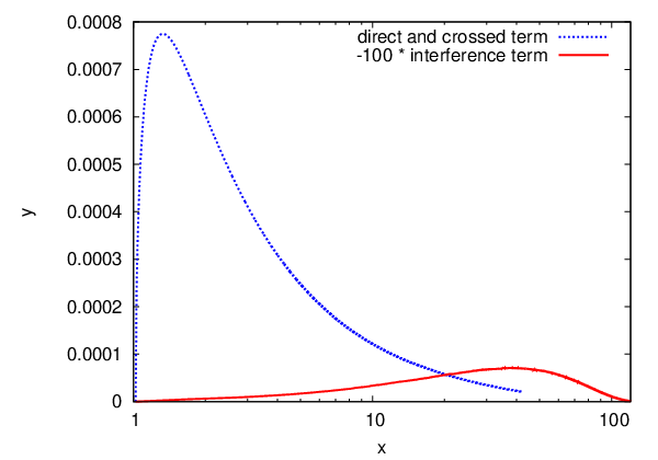
For the direct (crossed) term we can see a peak at very small
. The interference term in contrast is negative and wider. The different VMD
models give almost the same curves for the direct (crossed) and the
interference term. So we just plotted one curve, respectively. The errors
are smaller than the width of the lines.
The calculated values of the branching ratios are given in Table
4.6. The errors are again very small so that we do not show them.
| without VMD | hidden gauge | modified VMD | |
|---|---|---|---|
As one can see the contribution of the interference term () is of the order of one per cent
compared with the leading direct and crossed term (). Note that the
interference term has a negative
sign. The difference between the VMD models is very small for this
decay. We display four decimal places just to see a difference in the values
of the interference term. Moreover the errors are small. This is
compatible with the small
contribution of the VMD.
We can compare our results with other theoretical calculations and the
experimental data, see Table 4.7.
| [6] | [7] | [8] | [9] | Data [34] | |
|---|---|---|---|---|---|
| 3.47 | 3.29 |
For the case of the total rate we agree with all values of the recent references, namely
[6], [7],[8] and
[9]. Note that the comparison has to be done with the first column of Table 4.6, because
none of them used a vector meson dominance model. With respect to the interference
term, we totally agree with the values given in [8]. In
agreement with this reference we also differ by a factor of 5 compared with the result of Ref. [7]. All of
the predictions for the total branching ratio are consistent with the experimental data.
In the case of the , all three decays into two -pairs, two -pairs and an - plus a -pair are possible. The dependence of the differential branching ratio on the invariant masses can be seen in Figures 4.7 and 4.6.


The decay into two -pairs is similar to the analogous decay of the
. The errors are again smaller than the width of the line, but we can
see the difference between the used models. The curve without VMD is smaller
than the ones calculated with VMD models. For the direct and crossed term we
can also see a small difference between the hidden gauge and the modified VMD
model.
The graph for the decay into two -pairs is very different. We
do not need a logarithmic scale to present the values appropriately because
the direct and crossed terms are much wider. Also the amplitude is
smaller. The difference between the used models is obvious, even for the
interference term. For the first time we can see the errors in the direct and
crossed terms.


The differential ratio for the decay plotted versus has basically the same
structure than the decay into two -pairs. Here only the amplitude is
smaller. On the other hand, the differential ratio plotted versus is similar to the decay into two -pairs, with
bigger and wider amplitude.
Now we present our results of the branching ratios for these three
decays, calculated without VMD, with the hidden gauge, and
with the modified model, and compare them with other theoretical values
as well as the experimental data (Table 4.8).
| without VMD | hidden gauge | modified VMD | [7] | [9] | Data [34] | |
| 6.26 | ||||||
| 1.48 | ||||||
| 4.27 | ||||||
The relative branching ratio of the -decay is much smaller
than the branching ratios of the other 4-lepton decays. This is caused by the very small
phase space in this reaction. The interference term is again of the order of
one per
cent.
In Ref. [77] the decays
and were
calculated with VMD models and without. These values
totally agree with ours.
Our values of the decays and calculated without a VMD form factor approximately agree with the results given in
[7]. The difference may be caused by the improved input data
that we
used. We also agree with [9] for the -decay
while their values for are much smaller. We
disagree again for the values of the interference term. Our interference term
is here about 10 times smaller than the values given in
[7]. Ref. [9] did not calculate an
interference term. We also disagree in the total branching ratio of the
decay , but the factor 2 of [7] may be due to a
typographical error in their calculations. This was already pointed out by the
authors of [8], when they compared the respective results of the decay
. It is clearly visible that Ref. [9] gives even
smaller values than [7].
The vector meson dominance factor now gives a big contribution. Especially for
the - and -decays this
factor is essential. While the results of the two VMD models are still very close to
each other, the one without VMD is distinctly
smaller. Unfortunately the existing experimental data only give upper bounds
which all of the models can meet. More precise measurements are needed to
falsify the VMD model.
Also for the case all three decay modes (, and ) are possible. The dependence of the branching ratios on the invariant mass is almost the same as in the analogous -decays. In general, the amplitudes in the -decays are greater. Also the differences between the VMD models are bigger. This holds also for the errors. Differences can be seen in the curve of the decay , where the width gives a very strong contribution to the branching ratio in the region of the vector meson mass when plotted against the invariant mass of the muons . This can be seen in Figure 4.8.

Plotted against the invariant mass
of the electrons one can not see the contribution of the width. Because of the
high mass of the muons the
energy of the electron pair does not get in the region of the vector meson mass.
In the curve of the decay the contribution of the width gives a small bend in the region of the
vector meson mass but this is hardly noticeable because the values in this area
are very small. Therefore we plotted the respective range in Figure 4.9.


For the decay again the width does not play a role, because the energy of the muons is lower than the vector meson mass. Therefore the dependence of the differential branching ratio on the invariant mass is similar to the one in the decay .
The branching ratios corresponding to the decays are given in Table 4.9.
| without VMD | hidden gauge | modified VMD | |
The contribution of the interference term is again of the same range. Because of the larger mass and thereby a bigger phase space, the
difference between the decay mode and the
other modes is smaller than for the -decays. We have again a huge effect of the
vector meson dominance factor for the case, and
even more so for the -decay. However, the theoretical and experimental status
is much worse than for the and cases, since no data exist.
Summary
In summary, the effect of VMD again increases with the value of the mass of the decaying particle and the lepton mass. It is very small for the case of the decay into four electrons and increases roughly by a factor of or , respectively, for the cases of the decay into four muons. The effect of the modified VMD model is noticeable, but not very large. A test whether a VMD model is needed or not and especially which version of the VMD model should be applied will be at least very difficult for these decay modes due to the lack of precise data.
4.3
The last of the decays via the triangle anomaly that we want to discuss is the one
of a pseudoscalar meson into a lepton pair . As mentioned in the
Chapter 3.2 a lot of work was done there before.
As discussed in Chapter 3 we can give a value for the subtraction constant
, see (3.56), which contains all of the nontrivial dynamics. The results calculated with the
hidden gauge model and the modified VMD model are compared to theoretical
values and experimental data in Table 4.10.
| hidden gauge | modified VMD | [12] | exp. data [78] | |
|---|---|---|---|---|
In [12] the authors presented the values of and the resulting
branching ratios calculated for various phenomenological models. All these
results basically fall into the same region (the predictions from the quark models
are even higher in absolute magnitude, varying between and ), higher in magnitude than the
experimental data. Our result matches very nicely the theoretical predictions,
but does not overlap with the experimental data.
This situation persists for the branching ratios of the decay . We present the unitary bound as discussed in Chapter 3 and also the branching ratios with respect to the total decay rate and the one into two photons in Table 4.11.
| unitary bound | hidden gauge | modified VMD | ||
|---|---|---|---|---|
For the decay an overview of theoretical predictions calculated via different models and a comparison with the latest KTeV result [78] can be found in [68], see Figure 4.10.

Most of these theoretical values can not describe the data
([78]) and this is the same for our calculations. The
values calculated via VMD models ([79, 66, 80]) are basically consistent with each other and
also with the values of modern calculations [12, 14]. The
overview contains calculations of ChPT
[81, 82, 83]. The calculated values of
[81] have very large uncertainties and are therefore the only
values, which can describe the data. The values given in
[82] and [83] have smaller uncertainties and
an overlap with the values of [81]. Though these values do not
overlap with each other. The authors of [82] provided a
consistent description of the decays , , and . According to [83] these
calculations did not take contributions of suppressed counterterms into account. In contrast the calculations of [83] contain
these contributions. Note that the values of [83] are
consistent with the values of VMD models and of modern calculations.
We will compare our results to the recent calculations given in [12]
and [14] and the existing experimental data explicitly, and also show
briefly the values of the various ChPT calculations.
The theoretical calculations of [12] and [14] and experimental data are given in Table 4.12.
| [12] | [14] | exp. data [78] | ||
|---|---|---|---|---|
Our calculated values agree with these theoretical
predictions. But although our value is a little bit higher, the theoretical
predictions are still approximately three standard deviations lower than the
experimental data.
The branching ratio calculated by [81] is the following:
| (4.2) |
As mentioned this value overlaps with the experimental data, but has a very large uncertainty. The braching ratio of [82] is
| (4.3) |
This value is higher than all other calculated values and also higher than the data. The values of [83] are given with respect to the decay into two photons and are consistent with our values:
| (4.4) |
We will now discuss the situation in the -sector. In addition to the decay also the decay is possible. Our calculated values are given in Table 4.13.
| unitary bound | hidden gauge | modified VMD | ||
|---|---|---|---|---|
We can compare our values to the theoretical ones and the experimental data, see Table 4.14.
| [12] | [14] | exp. data [34, 84, 16] | ||
|---|---|---|---|---|
Our results fall between the two different theoretical calculations given
in [12] and [14]. It is interesting to see
that the approach given in [14], which is a little bit closer to the
experimental data of the decay gives now worse predictions
for the decay if we compare it to the experimental
data. As in [12], we also reach a small
overlap with the experimental data. For the decay all
values meet the experimental bound.
The authors of [81] gave predictions for the decay :
| (4.5) |
One can see again the large theoretical uncertainty. The authors of Ref. [82] calculated this branching ratio as follows:
| (4.6) |
In Ref. [83] there are values given for both decays and :
| (4.7) |
The values of [83] are again consistent with our calculations.
The values of the -decays are given in Table 4.15. Experimental data do not exist.
| un. bound | hidden gauge | modified VMD | [12] | [14] | ||
|---|---|---|---|---|---|---|
| | 1.86 | |||||
| | ||||||
| | 1.30 | |||||
| |
It is remarkable that the branching ratio for the decay
is lower than the lower limit given by the unitary bound as can be seen in
our calculations and the ones of [14]. The reason is the
additional imaginary part which occurs because one of the intermediate vector mesons can go
on-shell. For the decays our calculated values are lower than both of
the other theoretical values.
In the sector there are only ChPT calculations done by [82]:
| (4.8) |
The branching ratio for the decay is very close to other theoretical values, while the one of is higher.
Summary
4.4 and
In this Section we will present the final results for the branching ratios of the
decays and for the
hidden gauge and the modified VMD model. There
exist several theoretical calculations ([22],
[19], [21]) and experimental
data ([34], [17], [16]), especially in the
sector, to compare with. We will also
give predictions for the CP violating terms and the electric terms. Finally an upper limit for the
model coefficient will be given.
and
We start with the dependence of the rate of the decay on the invariant mass of the decaying particle. We plot the leading (magnetic) term calculated, with the hidden gauge model and the modified VMD model, and the electric term which is scaled up to make it comparable (see Figures 4.11 and 4.12).


The behavior is quite similar to the graphs we showed before. With respect to
the dependence on
the invariant mass of the electrons, there is a large peak at low energies. The
behavior of the invariant mass dependence of the pions is much broader
with a smaller peak.
For the decay , the graphs are shown in Figures
4.13 and 4.14.


It is interesting that in these decays the electric terms seem to be much bigger
than in the previous case. But this is actually not the case if one compares the calculated values of the decay rates and branching ratios.
These values for the sector are listed in Table
4.16. Here the branching ratios relative to the total
decay width and to the width of the -decay are listed. The
asymmetry term is defined according to Eq. (2) of [23] with
the mixed term normalized to the total
width, see Eq. () of Chapter 3. The electric terms are independent of the various VMD models and
normalized to the total width.
| hidden gauge | modified VMD | ||
| 1.6 independent on VMD | |||
| 0.889 independent on VMD | |||
One can see that the branching ratio of is
much smaller than the other branching ratios. This is due to the smaller phase space. The
electric terms are about two orders of magnitude smaller for the decay and one order of magnitude smaller for the decay, even if we set to one. So it
is obvious that the magnetic terms still determines the leading
contribution. The difference in predictions of the various VMD models are
highly visible for the case of and the -decay. It is interesting that the CP-violating asymmetry term has a
negative sign. This is due to the negative sign of the VMD term relative to the
contact term. In the case of the magnetic term this term
appears squared, so it does not affect the sign there.
We can now compare our values with other data, see Table 4.16 and 4.17. Note that the authors of
[19] and [21] used the hidden gauge
model as well, while [22] calculated in the framework of unitary chiral
perturbation theory. So it will be more interesting to compare our values with
[22], because an agreement would be a verification of both models. The discrepancies between our values calculated via the hidden gauge model, and the ones given in
[19] for the and in
[21] for the decay can be
explained by the modern values of the constants , and as well as
the mixing angle. The data of [17] are the
most recent
published data and also the most interesting.
| [22] | [19], [21] | PDG [34] | KLOE [17] | ||
| 5.22 | |||||
For the -decay all theoretical values represent
the data very well. The modified VMD result is closer to
[22] than the hidden gauge result.
The decay is more interesting. One
can see by comparing Table 4.16 and 4.17 that the hidden gauge model does not agree with [22],
but that the modified model gives nearly the same value. The experimental situation
is even more interesting. The values of the hidden gauge model actually
represent the data of [34] better than the modified model,
although both are consistent. The recent data of the KLOE measurement
[17] are much smaller than the other experimental data and
also have extremely small errors. Neither other theoretical calculations [22] nor our values have an overlap. It would be very
interesting to see whether the measurement of the WASA@COSY experiment is compatible with
the one of KLOE, when their new data appear. (The most recent published data
of WASA@CELSIUS are already included in the PDG value and can be found in Ref.
[16].) If the data were confirmed a new theoretical view on this decay
channel would be needed.
The ratio is
relatively constant within the various VMD models, which makes sense, since
the VMD factors should approximately cancel. The errors are smaller because some prefactors cancel also. Note that our values are in agreement with
the ones of [22].
The comparison of this ratio to the recent KLOE data is again of special interest (see Table 4.18).
| PDG | ||||
|---|---|---|---|---|
Normalized to the PDG value the fraction is smaller than the theoretical predictions and has no overlap with these values.
The normalization to the recent CLEO data ([85]) gives a larger value, because the data of the CLEO experiment is smaller than the PDG value ().
This ratio has a small overlap with the UChPT value ([22]), as already pointed out in Ref. [17], but barely overlaps with our results.
Note that the PDG value does not include the CLEO data.
The PDG value is larger than all the other values. It has no overlap with any theoretical value. A measurement of this branching ratio in one experiment would be usefull.
We can now take a look at the CP violating asymmetry term
, see Eq. () of Chapter 3. Theoretically it was estimated by Ref. [23] as which is about half of our calculated value. was
measured for the first time via the forward-backward asymmetry by Ref.
[17]. According to these data we can give constraints for
the model coefficient . To make sure that our calculated values are
consistent with the KLOE data is has to be
| (4.9) |
This agrees with the assumption that is natural.
For the -decay, the choice of the VMD model does not have a
serious effect on the branching ratio, which is remarkable. Our values are
consistent with the ones of [22] and meet the upper
experimental bound easily.
and
In the curves of the differential decay rate of the decay there is a very strong contribution of the width as one can see in Figure 4.15. For the leading magnetic contribution the curve is shifted to the right for larger vector meson masses. The dependence of the asymmetry term is very interesting.


For the branching ratios the situation is somewhat different as we will discuss using the calculated values of the branching rations, see Table 4.19.
| hidden gauge | modified VMD | th. values [22] | exp. data [34] | ||
The calculation of the modified model now gives larger
values than the calculations of the hidden gauge model. We can see that the
CP violating terms are one order of magnitude lower than we the ones in the
-decays and are of positive sign. The electric terms
are visibly smaller than in the -decays. As we pointed out before we can assume
and so the electric terms do not have any effect.
In contrast to the -decay, the agreement of our values and the ones
of [22] does not hold any longer. For the and the channel the discrepancies are very small. However, for the
decay there is only a small overlap, although the
errors of [22] are very large.
Both of our VMD models as well as the values of [22] are
consistent with the data [34], though our values are less constraint by
the data. More precise measurements, especially for the
decay, are needed to see which model
represents the data the best.
Summary
For the decays the values calculated with the modified VMD model are closer to the experimental data. One can see that the modified model is indeed useful in the box anomaly sector. The lesser agreement for the -decays is due to the scarce data. This could also be the reason why the values of [22] are different especially for the decay . The asymmetry term was only measured for the decay . Although the errors given for the total branching ratios are extremely small, the ones for the asymmetry term are still much higher than the value itself. For the other decays we made predictions for the asymmetry term, which will be more accurate if the parameter can be given more precisely.
Chapter 5 Summary and outlook
In this work we studied anomalous decays of pseudoscalar mesons. We calculated explicit expressions for the decay rates and branching ratios and discussed the relevance of the form factors of the various vector meson dominance models. Thereafter, we presented our results of the branching ratios for the different vector meson dominance models and compared them to other theoretical values and experimental data.
For the decay our results represented the experimental data very well. Also the theoretical values calculated by other groups totally agreed with ours. The difference between the values calculated with and without VMD models was very pronounced for the decays . We were able to conclude that the VMD factor is needed here to represent the data, but we had no preference on one of the models. For the we also showed the contribution of the width.
The situation in the -channel was slightly different. Our values and the other presented theoretical values of the decay could represent the experimental data equally well. For the interference term we found differences to the results of the older calculations of [7] which had also been found by [8]. We calculated very different values for the decays in comparison to the other theoretical groups. We can refer again to [8] where an error in the calculations of [7] was found. Unfortunately experimental data are very scarce and only give upper bounds that all theoretical predictions could meet, so we could not constrain our results there. Theoretical calculations and experimental data for the respective -decays do not exist so that we could only make predictions. In the sector we also found contributions of the width in the decays and .
Our improvements in the case of were very limited. We basically followed the calculations of [12] and [14]. Our calculated values for the decay are very close to the ones they calculated and still far away from the experimental data. For the decays our results fall between the values of [12] and [14] and even have an overlap with the experimental data for the decay channel. The values for the decays are again very close to the ones of [12] and [14], but there exist no data to compare with.
In general, we found that the differences between the VMD models in the triangle anomaly sector are insignificant. This result is welcome, because the hidden gauge model could already describe the data very well.
In the box anomaly sector, we found that the modified VMD model led to improvements. The calculated values for the branching ratios of the decay represented the data very well for both VMD models, but the improved VMD model achieved a better agreement with the theoretical values calculated via unitary chiral perturbation theory ([22]). This was also valid for the decay . On the other hand the experimental situation is different, because the recent measurements done by KLOE supplied distinctly smaller values. Here the modified VMD model was closer to the experimental data and could almost reach an overlap. The calculated values for the decay matched with the ones of other theoretical calculations and met the upper experimental bound.
In the decay we also analyzed the CP-violating asymmetry term and compared our values to recent experimental data. We calculated an upper bound for the model specific factor . This factor scales a CP-violating, flavor-conserving local four-quark operator which is sensitive to the content of and and determines the strength of the additional electric form factor . We verified the claim that it could be of natural size. We also gave a prediction for the asymmetry term of the decay .
For the decays the situation was again different. The only existing
data were the ones of the decay . Here all models
represented the data very well. For the decay our
values were very different from the one calculated by
[22], but the experimental situation is too scarce that a
preference of any work can be justified. We found again very interesting contributions of the width in the sector. Especially for the asymmetry term we had a change in the algebraic sign in the region of the vector meson mass.
We completed the calculations concerning the anomalous decays of the and the in the framework of vector meson dominance. The only decays where the experimental data could not be described by theoretical calculations were the ones into two leptons and the decay . If the experimental data are confirmed, the probability that new physics is needed to describe the data is high indeed. The same holds for the decay , although the theoretical values and data are much closer than in the decay into two leptons.
The anomalous -decay should be investigated. The kinematics should be very similar to the ones of the decays , especially an interference term will contribute, but the form factor would be of special interest.
Appendix A Kinematics
A.1 The parallel boosts
Throughout we assume that all boosts are performed parallel (or anti-parallel) to the virtual- or real-photon axis which should point parallel to the -axis. Therefore only the and components of the 4-vectors will be affected by the boosts (e.g. and ), whereas the and components and will remain untouched. This is the reason for the notation and introduced in (2.49) and (2.50). Without loss of generality, we can therefore always mangage to rewrite (3.61) as
Note that the frames and boosts have been chosen in such a way that . Therefore, we always have
| (A.34) | |||
| (A.35) |
as it was applied in (A.1).
A.2 The relevant frames
The coordinates and four-momenta
in the rest frame are denoted here by a tilde (),
the ones
in the rest frame by an asterix (⋆), and the ones in the
rest frame by a
a diamond (⋄).
Thus, the relation (A.1) is given in the rest frame by
| (A.36) |
whereas in the rest frame it reads as
Switching the asterix (⋆) with a diamond (⋄) and with this relation holds in the rest frame.
A.3 Comparison with other kinematics
Note that is exactly the angle defined below Eq. (6) of Ref. [72]. Moreover, since the three-momentum of the meson in the rest frame is identical to the three-momentum in that frame (see (A.2)), the angle is identical to the angle defined below Eq. (1) of Ref. [23], i.e. identical to the angle between the three-momentum and the three-momentum in the rest frame:
| (A.76) |
Finally note
| (A.77) |
and in total analogy
| (A.78) |
See Ref.[23] for the definition of : i.e. is
the angle between the three-momentum and the three-momentum in the
rest frame. Note that the three-momentum in the
rest frame points into the negative -direction, therefore should be replaced
by if a common coordinate system (which involves ) is used.
Equations (A.76), (A.77) and (A.78) are the essential
formulae.
The kinematic of the decay is very close to the kinematics of the decay, the decay process of one kaon into two pions, one anti-lepton and one (to the lepton corresponding) neutrino, e.g.: The corresponding kinematics were introduced and described in Cabibbo and Maksymovicz [86], Pais and Treiman [87] and Bijnens et al. [71]. There is, however, one subtlety: the mass of the neutrino is of course assumed to be zero, whereas here both leptons have the non-vanishing mass . This induces changes in e.g. (A.89), (A.90) (A.94), (), (A.96) see below.
Refs. [86], [87] and [71] utilize the follwing five variables (see Fig. 1 of Ref. [86] or Fig. 5.1 of Ref. [71]) transcribed to the decay :

- 1.
- 2.
- 3.
- 4.
- 5.
Ref. [87] uses a convention for the metric opposite to the standard Bjorken-Drell metric.
The latter is applied here and in Refs.[86, 71].
Thus
and
In Ref. [86, 71] the following explicit construction can be found: Let v be a unit vector along the direction of flight of the in the rest frame (), i.e. . Furthermore, let c (d) a unit vector along the projection of () perpendicular to v (),
| c | (A.79) | ||||
| d | (A.80) |
Then one has
| (A.81) | |||||
| (A.82) | |||||
| (A.83) | |||||
| (A.84) | |||||
Thus .
A.4 Invariant expressions of the decay momenta
The interesting relations read:
| (A.85) | |||||
| (A.86) | |||||
| (A.87) | |||||
| (A.88) | |||||
| (A.89) | |||||
| (A.90) | |||||
| (A.91) | |||||
| (A.92) | |||||
| (A.93) | |||||
| (A.94) | |||||
| (A.96) |
Some of the relations given above deserve some additional remarks: Equation (A.92) can be rewritten as
| (A.97) |
It can be combined with correspondingly rewritten equation (A.93)
| (A.98) | |||||
such that the following relations hold:
| (A.99) | |||||
| (A.100) | |||||
| (A.101) | |||||
| (A.102) |
Note that these expressions deviate from Eqs.(10) and (11) of Ref. [23], where
there is a factor instead of in front of .
In fact, the normalization of Eq. (A.98) exactly agrees with the normalization
of the first relation of Eq. (3) from Ref. [87], when Eqs. (2’) and (3’) of that reference
are inserted into this relation.
Using (A.94) and () we will get the following expressions:
In order to derive the relation () we used the relation
| (A.104) |
This expression can be calculated via
The zero component can be expressed via (A.92) and
(A.94) to
| (A.105) |
With this relations we can calculate the expression
| (A.106) |
which is essential for the structure of ().
Finally we list the scalar products:
A.5 Projection tensor
The projection tensor, which we needed in Chapter 3, can be constructed via the summation over the final spins and of the current
| (A.108) | |||||
A.6 Decay rate
We will now discuss the decay rate for a decay of a particle with momentum
into four particles with momenta and . The
notation of the particles follows the ones of the momenta. The decay rates into two and three particles are also
given, (A.112) and (A.113).
The decay rate is defined as follows:
| (A.109) |
with the four body phase space:
is the matrix element squared.
We investigate the case where decays into three particles with momenta and , where the third particle , in our decay it is always a (off-shell) photon, decays into the remaining two particles via a two-body decay:
| (A.111) |
with the following expressions for the two body and three body decays [34]:
| (A.112) |
| (A.113) |
The decay rate becomes
| (A.114) |
The angles are defined as ; is the solid angle of the
in the rest frame, is the angle of
in the rest frame; and is the angle of in the rest frame.
We use the relation
in the integration. The momenta are the same as defined in the previous Section.
Because the squared matrix element only contains the angles
, and we can integrate over the
remaining angles. Therefore, we combine the azimuthal angles of and to the corresponding
angle as the difference between the planes and integrate over the
remaining independent angle in Fig. A.1. The angles stay untouched and can be
integrated out.
The decay rate becomes
| (A.115) |
Appendix B Translation formulae for the mixed and interference term of the decay
Most of the expressions are invariant and independent of the different rest frames and therefore easy to be calculated in terms of the equations given in Appendix A:
| (B.1) | |||
| (B.2) |
Using the above expressions, one can easily
calculate as well as and .
The expressions for the angles ,
and are more complicated, but can also be given
in terms of the invariants:
| (B.3) | |||
| (B.4) | |||
| (B.5) |
Appendix C Further calculations for the decay
C.1 Numerator of the amplitude Eq. (3.48)
To calculate the numerator of the Integral in we first deal with in (3.48). This form is rather unusual, because normally the completeness relations have a form with the same particle operator and the same momenta, e.g. . The derivation of such terms can be found in Appendix A of [64]. Therefore we calculate structures with different momenta first and insert the different operators via the expressions , respectively, . A general form for all structures is given in equation (A6) of that paper. Using this expressions general forms of projection operators on the singlet and triplet state of an outgoing lepton pair can be calculated. Because the total angular momentum of the lepton pair is it can only be either in a singlet or in a triplet state. The decaying particle is a pseudoscalar meson with and , such that . Since of the lepton pair is given by the outgoing lepton pair has to be in a singlet state to keep -invariance. We can now replace the term in (3.48) by the projector on the singlet state given in equation (A16) of [64]. This reads,
| (C.1) | |||||
where
| (C.2) |
were inserted. With this the amplitude changes to
| (C.3) |
is the singlet projection of the final lepton pair, which can be given by calculating the trace
| (C.4) |
Combining the remaining momenta and dealing with the two total antisymmetric tensors, we can derive
| (C.5) |
where we used the well known expression
| (C.6) |
C.2 Calculation of the imaginary part of the reduced amplitude
To calculate the imaginary part of the integral we use the rules of Cutkosky ([69]) where the off-shell propagators are replaced by -functions:
Moreover we switch to the rest frame of the decaying particle to rewrite its momentum as . The VMD part of course is equal to unity for on-shell photons. This leads to
| (C.7) |
We can now insert and rewrite the -functions
After integrating over spherical coordinates this reads
which is exactly the desired result
| (C.8) |
C.3 Derivation of the reduced amplitude
We will give the derivation of the subtraction constant following the work of [13]. To evaluate the amplitude we first transform the integral from Minkowski to Euclidean space by . Now we will rewrite the VMD form factor in terms of a double Mellin transformation. According to e.g. [88] a Mellin transformation is defined as
| (C.9) |
with the inverse Mellin transformation given as
| (C.10) |
So, the double-mellin-transformed form factor is given by
| (C.11) |
Here is the characteristic scale for the form factor, in our case the vector meson mass , , the vector , and is the inverse Mellin transform of the VMD form factor given as
| (C.12) |
The integral (3.51) can be rewritten using Feynman parameters. Therefore the denominator reads (see e.g. equation (6.42) of [38]):
| (C.13) | |||||
with . Applying this we can calculate the loop integral:
| (C.14) | |||||
Using the Mellin transformed form factor and the loop integral (C.14) this leads to [13]
| (C.15) | |||||
Because we are only interested in we set . Using again equation (6.42) of [38] to integrate over the Feynman parameters and setting and this reads
| (C.16) | |||||
The integral can be solved, as in [13],with the help of the residues:
| (C.17) |
The authors of [13] followed the work of [89] and found two contributions to the integral according to the residues
| (C.18) |
| (C.19) |
They give the following contributions to the integral [13]:
| (C.20) | |||||
| (C.21) | |||||
| (C.22) |
We need to give expressions for the Mellin transformed form factor. This can be done using Mellin transforms of derivatives as mentioned in Chapter 4.2 of [88]. It can be proven that the following relation holds:
| (C.23) |
Here denotes the derivatives of order of with respect to the corresponding arguments of the form factor. Thus the following relation obviously holds:
| (C.24) |
Setting we can easily integrate over :
| (C.25) | |||||
In the last step we used , which is obviously the case for our VMD form factor. If we extend this relations to two arguments of , we can now give the following expressions for the Mellin-transformed VMD form factors [13].
| (C.26) |
Inserting (C.26) in (C.21) and (C.22) one gets the following result:
This can be expanded in , and in the limit we get
| (C.28) | |||||
To the lowest order of one gets the desired result [13]
| (C.29) |
To the next order one finds:
| (C.30) |
Bibliography
- [1] N. P. Samios, Phys. Rev. 121, 275 (1961).
- [2] Y. A. Budagov, S. Viktor, V. P. Dzhelepov, and P. F. Ermolov, Sov. Phys. JETP 11, 755 (1960).
- [3] D. W. Joseph, Nuovo Cim. 16, 997 (1960).
- [4] A. Beddall and A. Beddall, Eur. Phys. J. C54, 365 (2008).
- [5] L. G. Landsberg, Phys. Rept. 128, 301 (1985).
- [6] N. M. Kroll and W. Wada, Phys. Rev. 98, 1355 (1955).
- [7] T. Miyazaki and E. Takasugi, Phys. Rev. D8, 2051 (1973).
- [8] A. R. Barker, H. Huang, P. A. Toale, and J. Engle, Phys. Rev. D67, 033008 (2003), hep-ph/0210174.
- [9] C.-C. Lih, (2009), 0912.2147.
- [10] A. Deshpande et al., Phys. Rev. Lett. 71, 27 (1993).
- [11] K. S. McFarland et al., Phys. Rev. Lett. 71, 31 (1993).
- [12] A. E. Dorokhov and M. A. Ivanov, Phys. Rev. D75, 114007 (2007), 0704.3498.
- [13] A. E. Dorokhov and M. A. Ivanov, JETP Lett. 87, 531 (2008), 0803.4493.
- [14] A. E. Dorokhov, M. A. Ivanov, and S. G. Kovalenko, Phys. Lett. B677, 145 (2009), 0903.4249.
- [15] KTeV, E. Abouzaid et al., Phys. Rev. Lett. 100, 182001 (2008), 0802.2064.
- [16] M. Berlowski et al., Phys. Rev. D77, 032004 (2008).
- [17] KLOE, F. Ambrosino et al., (2008), 0812.4830.
- [18] CMD-2, R. R. Akhmetshin et al., Phys. Lett. B501, 191 (2001), hep-ex/0012039.
- [19] C. Picciotto, Phys. Rev. D45, 1569 (1992).
- [20] C. Q. Geng, C. C. Lih, and W.-M. Zhang, Phys. Rev. D62, 074017 (2000), hep-ph/0007252.
- [21] C. Picciotto and S. Richardson, Phys. Rev. D48, 3395 (1993).
- [22] R. Nissler and B. Borasoy, AIP Conf. Proc. 950, 188 (2007).
- [23] D.-N. Gao, Mod. Phys. Lett. A17, 1583 (2002), hep-ph/0202002.
- [24] J. Wess and B. Zumino, Phys. Lett. B37, 95 (1971).
- [25] E. Witten, Nucl. Phys. B223, 422 (1983).
- [26] M. Bando, T. Kugo, and K. Yamawaki, Prog. Theor. Phys. 73, 1541 (1985).
- [27] T. Fujiwara, T. Kugo, H. Terao, S. Uehara, and K. Yamawaki, Prog. Theor. Phys. 73, 926 (1985).
- [28] U.-G. Meißner, N. Kaiser, A. Wirzba, and W. Weise, Phys. Rev. Lett. 57, 1676 (1986).
- [29] M. Benayoun, P. David, L. DelBuono, O. Leitner, and H. B. O’Connell, Eur. Phys. J. C55, 199 (2008), 0711.4482.
- [30] M. Benayoun, P. David, L. DelBuono, and O. Leitner, Eur. Phys. J. C65, 211 (2010), 0907.4047.
- [31] M. Benayoun, P. David, L. DelBuono, and O. Leitner, (2009), 0907.5603.
- [32] B. R. Holstein, Phys. Scripta T99, 55 (2002), hep-ph/0112150.
- [33] Particle Data Group, G. P. Yost et al., Phys. Lett. B204, 1 (1988).
- [34] Particle Data Group, C. Amsler et al., Phys. Lett. B667, 1 (2008).
- [35] S. L. Adler, Phys. Rev. 177, 2426 (1969).
- [36] J. S. Bell and R. Jackiw, Nuovo Cim. A60, 47 (1969).
- [37] K. Fujikawa, Phys. Rev. Lett. 42, 1195 (1979).
- [38] M. E. Peskin and D. V. Schroeder, Reading, USA: Addison-Wesley (1995) 842 p.
- [39] J. D. Bjorken and S. D. Drell, Bibliograph.Inst./Mannheim 1967, 409 P.(B.I.- Hochschultaschenbücher, Band 101).
- [40] O. Kaymakcalan, S. Rajeev, and J. Schechter, Phys. Rev. D30, 594 (1984).
- [41] H. Gomm, O. Kaymakcalan, and J. Schechter, Phys. Rev. D30, 2345 (1984).
- [42] O. Kaymakcalan and J. Schechter, Phys. Rev. D31, 1109 (1985).
- [43] P. Jain, N. W. Park, J. Schechter, R. Johnson, and U.-G. Meißner, In *Storrs 1988, Proceedings, 4th Meeting of the Division of Particles and Fields of the APS* 587-589.
- [44] M. Bando, T. Kugo, and K. Yamawaki, Nucl. Phys. B259, 493 (1985).
- [45] U.-G. Meißner, Phys. Rept. 161, 213 (1988).
- [46] M. Harada and K. Yamawaki, Phys. Rept. 381, 1 (2003), hep-ph/0302103.
- [47] K. Kawarabayashi and M. Suzuki, Phys. Rev. Lett. 16, 255 (1966).
- [48] Riazuddin and Fayyazuddin, Phys. Rev. 147, 1071 (1966).
- [49] J. J. Sakurai, Annals Phys. 11, 1 (1960).
- [50] M. Bando, T. Kugo, and K. Yamawaki, Phys. Rept. 164, 217 (1988).
- [51] S.-Y. Furui, R. Kobayashi, and K. Ujiie, Prog. Theor. Phys. 76, 963 (1986).
- [52] P. Jain, R. Johnson, U.-G. Meißner, N. W. Park, and J. Schechter, Phys. Rev. D37, 3252 (1988).
- [53] J. Bijnens, A. Bramon, and F. Cornet, Phys. Rev. Lett. 61, 1453 (1988).
- [54] L. Ametller, Phys. Scripta T99, 45 (2002), hep-ph/0111278.
- [55] J. L. Goity, A. M. Bernstein, and B. R. Holstein, Phys. Rev. D 66, 076014 (2002).
- [56] B. Moussallam, Phys. Rev. D 51, 4939 (1995).
- [57] B. L. Ioffe and A. G. Oganesian, Phys. Lett. B647, 389 (2007), hep-ph/0701077.
- [58] Prim Ex, M. Kubantsev, I. Larin, and A. Gasparyan, (2006), physics/0609201v1.
- [59] T. E. O. Ericson and W. Weise, Oxford, UK: Clarendon (1988) 479 P. (The International Series of Monographs on Physics, 74).
- [60] C. Itzykson and J. B. Zuber, New York, USA: McGraw-Hill (1980) 705 P.(International Series In Pure and Applied Physics).
- [61] J. A. M. Vermaseren, (2000), math-ph/0010025.
- [62] B.-Y. Young, Phys. Rev. 161, 1620 (1967).
- [63] M. Pratap and J. Smith, Phys. Rev. D5, 2020 (1972).
- [64] B. R. Martin, E. De Rafael, and J. Smith, Phys. Rev. D2, 179 (1970).
- [65] L. Bergstrom, Zeit. Phys. C14, 129 (1982).
- [66] L. Bergstrom, E. Masso, L. Ametller, and A. Bramon, Phys. Lett. B126, 117 (1983).
- [67] Z. K. Silagadze, Phys. Rev. D74, 054003 (2006), hep-ph/0606284.
- [68] A. E. Dorokhov, Nucl. Phys. Proc. Suppl. 181-182, 37 (2008), 0805.0994.
- [69] R. E. Cutkosky, J. Math. Phys. 1, 429 (1960).
- [70] S. Mandelstam, Phys. Rev. 115, 1741 (1959).
- [71] J. Bijnens, G. Colangelo, G. Ecker, and J. Gasser, (1994), hep-ph/9411311.
- [72] C. Q. Geng, J. N. Ng, and T. H. Wu, Mod. Phys. Lett. A17, 1489 (2002), hep-ph/0201191.
- [73] M. Gorchtein, (2008), 0803.2906.
- [74] C. Q. Geng, C. C. Lih, and W.-M. Zhang, Phys. Rev. D57, 5697 (1998), hep-ph/9710323.
- [75] A. A. Poblaguev, Phys. Lett. B238, 108 (1990).
- [76] CERNLIB, http://cernlib.web.cern.ch/cernlib/ .
- [77] J. Bijnens and F. Perrsson, (1999), hep-ph/0106130.
- [78] KTeV, E. Abouzaid et al., Phys. Rev. D75, 012004 (2007), hep-ex/0610072.
- [79] K. S. Babu and E. Ma, Phys. Lett. B119, 449 (1982).
- [80] L. Ametller, A. Bramon, and E. Masso, Phys. Rev. D48, 3388 (1993), hep-ph/9302304.
- [81] M. J. Savage, M. E. Luke, and M. B. Wise, Phys. Lett. B291, 481 (1992), hep-ph/9207233.
- [82] D. Gomez Dumm and A. Pich, Phys. Rev. Lett. 80, 4633 (1998), hep-ph/9801298.
- [83] M. Knecht, S. Peris, M. Perrottet, and E. de Rafael, Phys. Rev. Lett. 83, 5230 (1999), hep-ph/9908283.
- [84] R. Abegg et al., Phys. Rev. D50, 92 (1994).
- [85] CLEO, A. Lopez et al., Phys. Rev. Lett. 99, 122001 (2007), 0707.1601.
- [86] N. Cabibbo and A. Maksymowicz, Phys. Rev. 137, B438 (1965).
- [87] A. Pais and S. B. Treiman, Phys. Rev. 168, 1858 (1968).
- [88] I. H. Sneddon, McGraw-Hill, Inc (1972).
- [89] M. Passare, A. K. Tsikh, and A. A. Cheshel, Theor. Math. Phys. 109, 1544 (1997), hep-th/9609215.