Conditions for Correct Sensor Network Localization
Using SDP Relaxation
Abstract
A Semidefinite Programming (SDP) relaxation is an effective computational method to solve a Sensor Network Localization problem, which attempts to determine the locations of a group of sensors given the distances between some of them. In this paper, we analyze and determine new sufficient conditions and formulations that guarantee that the SDP relaxation is exact, i.e., gives the correct solution. These conditions can be useful for designing sensor networks and managing connectivities in practice.
Our main contribution is threefold: First, we present the first non-asymptotic bound on the connectivity (or radio) range requirement of randomly distributed sensors in order to ensure the network is uniquely localizable with high probability. Determining this range is a key component in the design of sensor networks, and we provide a result that leads to a correct localization of each sensor, for any number of sensors. Second, we introduce a new class of graphs that can always be correctly localized by an SDP relaxation. Specifically, we show that adding a simple objective function to the SDP relaxation model will ensure that the solution is correct when applied to a triangulation graph. Since triangulation graphs are very sparse, this is informationally efficient, requiring an almost minimal amount of distance information. Finally, we analyze a number of objective functions for the SDP relaxation to solve the localization problem for a general graph.
1 Introduction
Graph Realization is a commonly studied topic which attempts to map the nodes in a graph to point locations in Euclidean space based on the non-negative weights of the edges in ; that is, the weight of each edge corresponds to the Euclidean distance between the incident points. There are a number of applications of the graph realization problem [9, 13, 16, 25, 21]. In this paper, we focus on the application to Sensor Network Localization (SNL).
A sensor network consists of a collection of sensors whose locations are unknown, and anchors whose locations are known. A common property of a sensor network is that each sensor detects others within a given connectivity (or radio) range and determines the distance from itself to these nearby sensors. Given this set of known distances, the goal is to determine the exact location of each sensor. The problem becomes a graph realization problem by forming the weighted undirected graph , where the node set represents the sensors and each non-negative weighted edge in represents a known distance between two sensors.
The SNL problem has received a lot of attention recently because of the formulation of its relaxation as a Semidefinite Program (SDP) [11, 30, 2, 24]. This formulation can find the exact locations of the sensors, given that the graph possesses certain properties.
Definition 1
A correct localization, or a correct solution, provides a set of points that is exactly equal to the sensor locations. That is, the solution not only solves a given formulation, but it provides the correct sensor locations in the desired dimension.
In this paper, we present a number of additional sufficient conditions that guarantee unique localizability (and hence a correct localization) of the SDP relaxation of the SNL problem. These conditions can be useful for designing sensor networks and managing connectivities in practice.
1.1 Background
We are given a graph in a fixed dimension , where the nodes, or points, of are partitioned into two sets: the set of anchors (where ) whose locations are known and the set of sensors, whose locations are unknown. The edge set also consists of two distinct sets: the set of edges between sensors, and the set of edges between an anchor and a sensor. Moreover, for each (or ) the Euclidean distance between sensor and sensor (respectively, anchor and sensor ) is known as (respectively ). The problem of finding the locations of the sensors can be formulated as finding points that satisfy a set of quadratic equations:
| (SNL-norm) |
From this, a number of fundamental questions naturally arise: Is there a localization or realization of ’s that solves this system? If there is a solution, is it unique? And is there a way to certify that a solution is unique? Is the network instance partially localizable, i.e., is the localization solution for a subset of the sensors unique? These questions were extensively studied in the graph rigidity and discrete geometry communities from a more combinatorial and theoretical prospective (see [20, 15] and references therein). However, the question of whether there is an efficient algorithm to numerically answer some of these questions remains open.
The SDP relaxation model (SNL-SDP) and corresponding method aim to answer these questions computationally (see [11, 30]). Let represent the th column of the identity matrix in , and define the symmetric matrices and , where is the vector of all zeros. The SDP relaxation can be represented as:
| (SNL-SDP) |
Here, represents the upper-left -dimensional principle submatrix of , the matrix dot-product refers to the sum of element-wise products , and means that the symmetric variable matrix is positive semidefinite. Note that problem (SNL-SDP) is a convex semidefinite program and can be approximately solved in polynomial time by interior-point algorithms.
One can see that the solution matrix of (SNL-SDP) is a matrix that can be decomposed into submatrices,
The constraint holds if and only if . If , then the above formulation finds a matrix such that the columns of its submatrix satisfy all quadratic equations in (SNL-norm).
Definition 2
Note that the notion of unique localizability is stronger than the notion of global rigidity. A sensor network is globally rigid only if there is a unique that satisfies (SNL-norm), but it may also have a solution in a higher dimension space, that is a nontrivial extension of , which satisfies (SNL-norm) [30, 1].
The following theorem was proved in [30]:
Theorem 1
The theorem asserts that the certification of a uniquely localizable network instance can be achieved by solving a convex optimization problem; the proof is constructive and produces a unique realization or localization solution for the original problem (SNL-norm).
The dual of the SDP relaxation (SNL-SDP)
| minimize | ||||
| subject to | (SDP-dual) |
is also useful, in that the solution to the dual tells us key properties about the primal. We define the dual slack matrix as
for . The dual slack matrix is optimal if and only if it is feasible and meets the complementarity condition, . If complementarity holds, then rank rank, and since rank, this means that rank. Thus, if an optimal dual slack matrix has rank , then every solution to (SNL-SDP) has rank [30]. In fact, we have a stronger notion on localizability:
Definition 3
A sensor network is strongly localizable if there exists an optimal dual slack matrix with rank .
Again, such a max-rank dual solution matrix can be computed approximately in polynomial time using SDP interior-point algorithms.
1.2 Our Contributions
In this paper, we present new conditions that guarantee unique localizability of the SDP relaxation of the problem, i.e., conditions that ensure the SDP will give the correct solution so that the sensor network can be localized in polynomial time. We also enhance the relaxation such that the new SDP relaxation will produce a correct solution in dimension to satisfy (SNL-norm), even when the standard SDP relaxation (SNL-SDP) may not. More precisely, our result is twofold:
- 1.
A very popular graph in the context of sensor network localization is the unit-disk graph, where any two sensor points (or a sensor point and an anchor point) are connected if and only if their Euclidean distance is less than a given connectivity radius . It has been observed that when the radius (or radio range) increases, more sensors in the network can be correctly localized. There is an asymptotic analysis to explain this phenomenon when the sensor points are uniformly distributed in a unit-square [3]. In this paper, we present a non-asymptotic bound on the radius requirement of the points in order to ensure the network is uniquely localizable with high probability. Specifically, we decompose the area into sub-regions, which allows us to analyze whether the locations of points in each sub-region can be determined, as opposed to analyzing each point individually. We then determine the probability that the locations of all sensors can be determined, given a specified concentration of the sensors in a given area. This may have practical impact by providing guidance on communication power ranges that ensure the network is uniquely localizable.
- 2.
The basic SDP localization model (SNL-SDP) is an SDP feasibility problem. An open question has been to determine whether adding a certain objective function to the basic model improves localizability of the problem; that is, if the SDP feasible region contains high-rank solutions, is the SDP optimal solution guaranteed to be unique and low-rank with a certain objective? We give an affirmative answer for a generic class of graphs, by identifying an objective function that will always result in a correct localization for this class of graphs. Our result may also have an influence on Compressed Sensing, which uses an objective function to produce the sparsest solution. Based on this idea, we present numerical results by comparing several SDP objective functions to illustrate their effectiveness.
Moreover, although our theoretical analyses are based on exact distance measurements, similar extensions of our model (established in earlier SDP work) would be applicable to noisy distance data.
1.3 Paper Organization
The organization of this paper is as follows. First, Section 2 derives a lower bound for the connectivity radius in a sensor network that guarantees unique localizability with high probability. In Section 3, we prove that given a triangulation (i.e., a planar, chordal and convex) graph, if the sum of the distances between nodes that do not have an edge between them is maximized, then the graph will be strongly localizable. We use this idea, and test a number of heuristic objective functions on a large number of random sensor networks to determine how well each works in practice. Our results for these heuristics are presented in Section 4.
2 Bounding the Connectivity Radius
In this section, we consider the unit-disk graph model [7, 8, 14] for sensor networks, where the Euclidean distance between any two sensor points (or a sensor point and an anchor point) is known (i.e., the two points are connected) if and only if the distance between them is less than a given connectivity radius . Assuming that the sensor points are randomly distributed in a region, we then establish a lower bound on radius that guarantees unique localizability, with high probability, of the sensor network formed based on radius . We do this by establishing a lower bound on radius to ensure that the unit-disk graph is a -lateration graph, which is a sufficient condition for unique localizability.
Definition 4
For some , the graph is a (+1)-lateration graph if there exists a permutation of the points, , such that the edges of the sub-graph form a complete graph, and each successive point for is connected to points in the set . This permutation of the points, , is called a -lateration ordering.
It is shown in [35] that if a sensor network graph contains a spanning -lateration graph and the points are in general position, then it is uniquely localizable. Zhu et al. [35] provide a rigorous proof, which is based on the intuitive concept that given points in general position forming a complete graph, the locations of the points can be always be uniquely determined, and the location of any point connected to points with known locations can also be determined.
Define to be the smallest connectivity radius of the randomly distributed sensor points that ensures the network is uniquely localizable with probability at least . To find a lower bound on , we can find a connectivity radius for which the unit-disk graph will contain a spanning -lateration graph with at least probability .
We approach the problem by considering a unit hypercube , which contains all the sensor points. We then split the region into a grid of equal sub-hypercubes in dimension , say , where each sub-hypercube will have a volume of , and the length of each of its edges will be . Without loss of generality, we can assume , where is a positive integer and . Similarly, if the region considered is a hyper-rectangle in dimension , we can assume , where for are positive integers. This partition will allow us to analyze the probability that the locations of sensors in a given region can be determined, as opposed to analyzing each individual point.
2.1 Ensuring a Clique in the Graph
Since a -lateration ordering on the points must begin with a -clique, we first find a lower bound on the radius to ensure there exists at least one clique of points in the graph.
Proposition 1
Let contain points, and and (or equivalently ). Then, there exists at least one clique of points in the unit-disk graph .
Proof: Note that is the length of the diagonal of each sub-hypercube . Thus, if is lower-bounded by the given value, then every point in a sub-hypercube will be connected to any other point in the same sub-hypercube. Furthermore, since there are at most sub-hypercubes, by the pigeon-hole principle, at least one of them contains at least points and they must form a clique of points in the unit-disk graph with given radius .
In what follows, we fix . We will initialize the spanning -lateration graph construction by choosing according to this lower bound, and let the points in the -clique be the first points in the lateration ordering. Since these points are randomly distributed, they must be in general position with probability one. Thus, we may assume that these points are anchors for the sensor network. This assumption is without loss of generality, because our bound on the radius established in the following sections will be much greater than the bound specified in Proposition 1, simply because we need to ensure that not only does there exist a clique of points, but also all sensor points in form a spanning -lateration graph with a high probability.
2.2 Binomial Distribution Model
One way to let the sensor points be randomly distributed throughout the area of is to let the points be binomially distributed throughout each sub-hypercube of . More specifically, the number of points, , placed in each sub-hypercube , for , will be independently and binomially generated according to with . Once is generated, we let these sensor points be arbitrarily placed in general position within sub-hypercube .
Using this binomial distribution model, let denote the total number of points in the hypercube . Since the values are independently and identically distributed and all sub-hypercubes are equally sized, the total number of points will be more or less evenly distributed in the entire hypercube . Furthermore, by properties of the binomial distribution,
Thus, almost surely and the assumption of binomially distributed sensor points throughout each sub-hypercube is statistically equivalent to assuming a uniform distribution of points throughout the whole region when is sufficiently large.
2.3 Connectivity Bound
We now form further conditions on the connectivity radius to ensure that the unit-disk graph contains a spanning -lateration graph. We have assumed that the points are binomially distributed in each sub-hypercube, parametrized as . First, must satisfy Proposition 1, since it ensures a ()-clique in . These points in the clique will represent the first points in the lateration ordering of a spanning -lateration graph (Definition 4).
We construct an improved bound on the probability of localizability through an ordering of the hypercubes, , and hence an ordering on the points. For simplicity, we prove the following lemmas for the case of , and we refer to the sub-hypercubes as sub-squares. We also refer to -lateration when as trilateration. However, we note that the same analysis can be applied to hypercubes in higher dimensions, and our bound in Lemmas 1–3 is analogous to the bound in dimension .
Lemma 1
Assume that each sub-square in has at least one point, and . If the points of three sub-squares in the same row in three consecutive columns are in the trilateration ordering, then the points in all sub-squares in those three columns are also in the ordering. Similarly, if the points in three consecutive sub-squares in the same column are in the trilateration ordering, then the points in all sub-squares in those three rows are also in the ordering.
Proof: First, note that the lower bound ensures that all points in a given sub-square are connected to all points in a neighboring sub-square, which share either an edge or a point within the given sub-square.
For ease of explanation, let represent the sub-square in the -th row and -th column, and consider the case that all points in the first three sub-squares in the first row of the grid are already in the trilateration. Since all points in sub-square are within the connectivity range of all three points in the first row, these points are in the trilateration. Then, all points in sub-square (or ) are within the connectivity range of at least three points in sub-square (or ), these points are also in the trilateration. Therefore, all points in the first three sub-squares of the second row are in the trilateration.
Similarly, all points in the third row of the grid in the first three columns are also in the trilateration. This pattern continues, until all points in the first three columns of the grid are in the trilateration.
A generalization of this shows that if there are three sub-squares in the same row and in consecutive columns with points in the trilateration, and each sub-square has at least one point, then all points in the corresponding columns are also in the trilateration.
An analogous result holds for three sub-squares in the same column and in consecutive rows.
Lemma 1 states that if there are three consecutive sub-squares in a row with points in the trilateration, then the trilateration ordering extends to all squares in the corresponding columns. This concept is used below in Lemma 2, which analyzes the cases depicted in Figure 1.


Lemma 2
Assume there is at least one point in each sub-square and . Then the associated unit-disk graph contains a spanning trilateration graph if either:
- a)
There is a -clique in a non-corner sub-square
- b)
There is a -clique in a corner sub-square and one of its neighbor squares has at least two points
Proof: Again, note that ensures all points in a given sub-square are connected to all points in neighboring sub-squares. We show that if either of the conditions of Lemma 2 are satisfied, then there exists a trilateration ordering on the points in the graph.
- a)
Consider the example in the left grid of Figure 1, where there is a -clique in the non-corner sub-square . Let the points in this clique be the initial points in the trilateration ordering. All points in the sub-squares are connected to this clique; let the points in these squares be next in the trilateration ordering.
By Lemma 1, all points in the sub-squares in rows 1-3 are in the trilateration ordering. Since there are at least three columns in , the same argument applies for the columns, and inductively, there is a trilateration ordering on the points that spreads throughout the entire hyperspace .
- b)
Now consider the right grid of Figure 1, where there is a -clique in the corner sub-square , and there are at least two points in a neighboring sub-square. Let the points in be the first points in the trilateration ordering. All points in the three sub-squares are connected to the points in the clique and hence in the trilateration ordering. Next, let the points in sub-squares be the succeeding points in the ordering. With a similar argument as before using Lemma 1, we can construct a trilateration on the points in the graph, and all points are in the trilateration.
Therefore, if the conditions of Lemma 2 hold, the
associated unit-disk graph contains a spanning trilateration graph.
The above lemma provides sufficient, but not necessary, conditions on a network for trilateration to exist, which implies unique localizability. Moreover, these are strict conditions for a sensor network, since the distribution of sensors in a network may not always ensure that there is one sensor in each sub-square. Thus, we extend these conditions to a more general case, and allow for the possibility of empty sub-squares. Clearly, too many empty sub-squares will result in a graph that is not uniquely localizable; also, if empty sub-squares exist, there must be restricting conditions to ensure the graph is not too sparse to ensure localizability. Thus, we establish additional properties of the graph that ensure a trilateration but allow for empty sub-squares.
Definition 5
Two neighboring sub-squares are called adjacent neighbors if they do not share any edges, but share a point; neighbors that share an edge are called simple neighbors. A sub-square is called densely surrounded if all its simple neighbors have at least two points and one of its simple neighbors has at least 3 points.

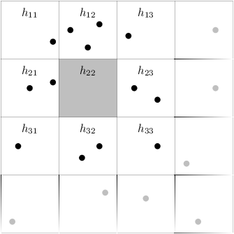
Lemma 3
Assume every empty sub-square is densely surrounded and . Then the associated unit-disk graph contains a spanning trilateration graph if there is a -clique in a non-corner sub-square.
Proof: Consider the grids in Figure 2, which shows an example and counter example of the conditions in Lemma 3.
- a)
First, consider the left grid of Figure 2, which does not satisfy the condition of Lemma 3 because there is a clique in a corner sub-square. Notice that if a trilateration ordering starts with the points in sub-square , it can continue to the points in sub-squares and , but will not spread to points in other sub-squares. That is, there is no trilateration ordering that starts with the points in and extends to the points in the sub-squares , because none of these sub-squares neighbor a subset of sub-squares, in the corresponding trilateration ordering, that contain at least 3 points combined. Thus, empty sub-squares must be densely surrounded to ensure a trilateration ordering on the points exists.
- b)
Now, consider the right grid of Figure 2, with a non-corner -clique, and a densely surrounded empty sub-square. This example shows the worst-case example of the condition in Lemma 3. The shaded sub-square is empty and densely surrounded, and the 3-clique is along the edge of the area . We prove that a trilateration ordering exists on the points in this sample grid with a densely surrounded sub-square. This proves Lemma 3 holds in the worst-case; the proof that Lemma 3 holds in every case is a generalized extension of this.
Define the permutation on the points in Figure 2 via the ordering on their sub-squares:
(1) This permutation is a trilateration ordering on the points in the sample grid. Note that is a trilateration ordering only because the sub-squares contain at least three points combined; that is, a permutation containing the points in the sub-squares can only be a trilateration if together contain at least three points.
Therefore, if the condition of Lemma 3 holds, the associated graph contains a spanning trilateration graph, and hence is uniquely localizable in dimension .
We now use the fact that a sensor network containing a spanning trilateration is uniquely localizable [35] to establish a lower bound on the probability that the unit disk sensor network with radius is localizable. Define the two events:
Then, the probability that a graph with such randomly distributed points is uniquely localizable will be
Given that the total number of sub-squares is (for some integer ), we introduce a parameter (or for general ) such that is the edge-length of each sub-square and we can use the same connectivity radius lower bound as before, now in terms of , . The distribution of point number in each sub-square is binomial , and there are a total of non-corner sub-squares in . Thus, the probability that there is a -clique in a non-corner sub-square is
Let be the number of empty sub-squares. By Lemma 2, , and if is the probability that one specific sub-square is empty, we have
Moreover, for any , we have
From Lemma 3, we know
The conditions of Lemma 3 require that empty sub-squares do not have empty simple neighbors; thus, we first find the probability that a sub-square does not have empty simple neighbors. Assume there are empty sub-squares, say . Because of the independence assumption, these empty sub-squares are uniformly distributed.
Given the empty sub-square , the probability that is not a simple neighbor of is at least ; the probability that is not a simple neighbor of or is at least ; and so on, so that the probability that no two empty sub-squares are neighbors is at least . Moreover, the probability that an empty sub-square is densely surrounded, i.e., that all simple neighbors of an empty sub-square have at least two points and at least one of them has more than two points, is:
Thus, the probability that all empty sub-squares are densely surrounded is
Note that the right hand side of the above equation is positive if . Thus, we only consider grids with less than empty squares. Finally, we have the lower bound given by the following expression:
| (2) |


For different values of (to be taken as the total number of sensor points), we can find values of , and thus (where can be viewed as the average number of sensor points in each sub-square), such that the right hand side of Equation (2) is at least . Figures 3a and 3b show and versus the number of points such that the right hand side of Equation 2 is at least .
We also compare our connectivity bound against the bound of Angulin et al. [3] in Figure 3. One can see that our bound and Angluin’s are almost identical for any value of . Thus, our result shows that the bound of Angluin et al. in (of for ) is true even when is small, although it was initially proved to be an asymptotic bound when is sufficiently large. Note that our bound, while not in an analytical form, is proved for any value of .
We recently learned of another asymptotic bound that was independently developed by Javanmard and Montanari [23]. However, this bound is much weaker than ours and Angluin’s.
Our connectivity result was proved for , i.e., the unit square in dimension . The result can be extended to dimension . In summary, we have the following Theorem 2.
Theorem 2
Let be the unit hypercube in dimension and be partitioned into a grid of equal sub-hypercubes, say , where is the edge length of each sub-hypercube. Let the number of sensor points in each sub-hypercube be independently and binomially generated according to where , and let one of the sub-hypercubes contain anchors. Then, if the connectivity radius satisfies , the probability that the sensor network is uniquely localizable is given by expression (2).
Again, the parameter of the binomial distribution can be viewed as the total number of sensor points in the region. We can also extend our result to another region in dimension into a grid of equal sub-hypercubes in dimension , say , where each sub-hypercube will have a volume of , and the length of each of its edges will be . For example, we can assume , where for are positive integers.
3 Unique Localization of Triangulation Graph
The basic SDP localization model (SNL-SDP) is an SDP feasibility problem. When the network is not uniquely localizable, the max-rank of SDP feasible solutions is strictly greater than . In practice, one may still be interested in finding a feasible SDP solution with rank , representing one possible localization of points in . In this section, we show that adding an objective function that maximizes the sum of certain distances in a triangulation graph (in ) will produce a rank- SDP solution. The result should be applicable to .
Definition 6
Consider a set of points . A triangulation, , of the points in is a subdivision of the convex hull of into simplices (triangles) , for some , such that the edges of two simplices do not intersect or share a common face.
Definition 7
For a triangulation , we define a triangulation graph such that and if and only if is an edge of a simplex in . Note that triangles in a triangulation graph do not overlap, and triangles do not exist strictly inside other triangles.
Triangulation graphs and their properties have been studied in the literature [12, 5, 26]. Bruck et al. [12] showed that embedding a unit disk graph with local angle information (angles between points) is NP-hard, while the same problem on a triangulation graph is not. Araújo and Rodrigues [5] introduced an algorithm to construct a triangulation graph from a unit disk graph with bit communications between points.


We formally decompose a triangulation into an initial clique and a set of actions , where an action consists of adding a point and connecting it to either two adjacent points or two connected external points, where a point is called external if it is not strictly inside the convex hull of a cycle in the graph. This leads us to the following lemma, whose proof is omitted.
Lemma 4
A triangulation can be constructed recursively by either adding an external point that connects to two adjacent points of a simplex (triangle) already in such that the new edges do not cross any existing edges (see Figure 4, 1-4), or simply connecting two external points already in to form a triangle (see Figure 4, 5).
Proof: By induction on an external point; see Figure 4.
Step 8 of Figure 4 shows the set of virtual edges in the sample triangulation graph. These virtual edges will be used to construct an appropriate objective function of the SDP relaxation for triangulation graphs.
Definition 8
In a triangulation graph, adjacent triangles are two triangles which share a common edge. A virtual edge exists between two points and when and belong to adjacent triangles, but . The set of virtual edges between sensors is denoted , and between sensors and anchors is denoted .
Consider adding an objective function to the SDP model (SNL-SDP) that maximizes the sum of the lengths of all virtual edges in a generic triangulation graph. The primal SDP relaxation, for , becomes:
| maximize | ||||
| subject to | ||||
| (3) | ||||
and the dual of (3) is:
| minimize | ||||
| subject to | ||||
| (4) | ||||
For a triangulation graph with at least three anchors, we can show that (4) is strictly feasible, i.e., there exists a feasible with (see Proposition 4.1. in [31]). The primal SDP (3) also has a feasible point. As a result, the strong duality and complementarity condition hold for (3) and (4).
We derive the following exact-localization theorem.
Theorem 3
Consider applying the SDP relaxation (3) to a generic triangulation graph with at least three anchors. Then, the rank of an optimal dual slack matrix of (4) is and the rank of the optimal SDP solution of (3) is , so that the pair is strictly complementary and the SDP relaxation produces the correct localization.
Proof: We use induction to show that the ranks of the optimal dual slack matrix and primal SDP solution are and , respectively. This implies that the strict complementarity conditions holds and (3) produces the correct localization, that is, the original true positions of the sensor points of the generic triangulation graph.
Assume the result is true for any triangulation graph with points. It remains to be shown that this also holds for graphs with points. It is clearly true for a single simplex when .
Let be the correct locations of points, where the superindex represents the number of points. By the induction assumption, the solution to (3) is . Moreover, the optimal dual slack matrix satisfies and has rank ; we can write the optimal dual slack matrix in terms of its submatrices , where and . Note that , which follows from the fact that rank and .
The complementarity condition means the elements of represent a stress on each edge such that the total force at all non-anchor points is zero (assuming, without loss of generality, a stress of on all virtual edges).
Definition 9
Given a set of sensor locations , let be the corresponding graph. A matrix is a stress matrix of the sensor network if it satisfies the constraints of (4) and . That is, each element of represents a stress on the associated edge in such that the total force on each non-anchor point is zero.
We decompose the triangulation graph into an initial simplex , and actions . Without loss of generality, we assume the points in the first triangle are anchor points and let the last points added to the graph be . For example, consider Figure 4; let be the dual slack matrix on points 1–7 and assume the subgraph induced on the first 7 points is uniquely localizable. When point 8 is added along with its incident edges, points form a clique (when including the virtual edge between 4 and 8, which is unique when its length is maximized). Consider an SDP relaxation problem in dimension 4 that maximizes the length of the virtual edge between 4 and 8; this problem will have a unique optimal solution with rank 2 that determines the exact location of points , and an optimal dual slack matrix that forms a stress matrix for these four points.
Now consider the general case, where is the last point added to the graph. A new triangle is created by adding , its adjacent triangle and the virtual edge, which forms a 4-clique. Let be the corresponding positive-semidefinite stress matrix on the graph formed by , the two points adjacent to (say, and ) and the point with which has a virtual edge (say, ). We examine the case where and are sensors, however the case where at least one of them is an anchor is an easy extension. As before, the locations , and can be uniquely determined by solving an SDP relaxation, and is the optimal dual slack matrix that solves its dual problem:
| minimize | (5) | |||
| subject to |
where
Assume is the optimal solution of this SDP, then
It’s easy to see that strong duality and complementarity condition hold for this SDP, and therefore
Note that because , and consider the updated stress matrix
where is the stress matrix of the new edges, that is, .
The new matrix will be feasible for the dual, since is the solution of (5), and , implies that .
Define
as the correct locations of the updated points. (Note that given this definition of , it does not immediately follow that rank, since the added last row of can be linearly independent from the first rows.) The sum of element-wise products of and is
Moreover, we can show that . Assume this is not true, i.e., assume that there is a vector such that
which holds if and only if and . Since , this means that the first elements of are zero, i.e., . Thus,
which implies . Thus, if and only if , implying and rank. Therefore, the rank of is , and consequently from [30], is the unique solution to (3), so that the localization is correct and exact.
Theorem 3 implies that the strict complementarity condition holds when localizing a generic triangulation graph with the selected objective function. This result is interesting because, in general, it is difficult to prove strict complementarity for SDPs. How to compute a stress matrix (or optimal dual matrix) and determine whether the stress matrix has rank are also important questions in rigidity theory for graph realization. Clearly, Theorem 3 is applicable to any graph that contains a generic triangulation graph as a spanning subgraph. In practice, the objective of the SDP relaxation may include all non-edges that are not specified in the given graph (rather than just virtual edges), which we experiment in the next section.
4 Heuristic Objective Function
Section 3 proves that adding a given objective function to (SNL-SDP) results in a correct localization for a certain class of graphs, whereas the formulation without an objective function may not.
Based on these findings, we tested a number of different SDP relaxation methods with different objective functions. For each method (i.e., each objective function), we ran the relaxation on a large number of random sensor networks and determined the success rate of each method. The following objective functions were tested to heuristically determine the best method.
- 1.
(ZERO) Solve the formulation (SNL-SDP) (with no objective function). This can be viewed as a control simulation against which to compare other methods.
- 2.
(MAX) Maximize the sum of all the ‘non-edge’ lengths by solving the formulation:
(SDP-MAX) - 3.
(MIN) Minimize the sum of all the ‘non-edge’ lengths by solving the formulation:
(SDP-MIN) - 4.
(MAX-PT) Maximize the sum of the distances from each sensor location to a distant point, where is set to the corresponding elements of the decision matrix . For example, for the vector of all ones, we took the point and solved the formulation:
We constructed 200 uniformly distributed sensor networks and tested each method on the networks for a number of different radio ranges. Each randomly distributed sensor network has 100 points in a unit square (in dimension ), and the distance between two points is known when they are within the given radio range. Table 1 shows the percent of sensor networks that were correctly localized using each method, for each radio range.
| Method | |||||
|---|---|---|---|---|---|
| ZERO | MAX | MIN | MAX-PT | ||
| Radio Range | 0.15 | 0 | 0 | 0 | 0 |
| 0.2 | 41 | 75 | 39 | 0 | |
| 0.25 | 87 | 95 | 88 | 0 | |
| 0.3 | 98 | 100 | 100 | 4 | |
| 0.35 | 100 | 100 | 100 | 7 | |
| 0.4 | 100 | 100 | 100 | 13 | |
As can be seen from Table 1, maximizing the sum of the unknown distances out-performs the other three methods tested, and maximizing the sum of distances from a distant point does not produce good results. Moreover, the methods (ZERO), (MAX) and (MIN) all seemed to work very well when the radio range was at least 0.35. This radio range is much smaller than the lower bound given by (2), but has not been theoretically proved as a radio range that will lead to a correct localization.
References
- [1] A. Y. Alfakih. On the universal rigidity of generic bar frameworks. Contribution to Discrete Mathematics, 5(3):7–17, 2010.
- [2] A. Y. Alfakih, A. Khandani, and H. Wolkowicz. Solving euclidean distance matrix completion problems via semidefinite programming. In Computational Optimization and Applications, volume 12, pages 13–30, 1999.
- [3] D. Angluin, J. Aspnes, M. Chan, M. J. Fischer, H. Jiang, and R. Peralta. Stably computable properties of network graphs. In V. K. Prasanna, S. Iyengar, P. Spirakis, and M. Welsh, editors, Distributed Computing in Sensor Systems: First IEEE International Conference, DCOSS 2005, Marina del Rey, CA, USE, June/July, 2005, Proceedings, volume 3560 of Lecture Notes in Computer Science, pages 63–74. Springer-Verlag, June 2005.
- [4] D. Angluin, J. Aspnes, Z. Diamadi, M. J. Fischer, and R. Peralta. Computation in networks of passively mobile finite-state sensors. Distributed Computing, pages 235–253, March 2006.
- [5] F. Araújo and L. Rodrigues. Fast localized delaunay triangulation. volume 3544, pages 81–93. Principles of Distributed Systems, 2005.
- [6] J. Aspnes, T. Eren, D. K. Goldenberg, A. S. Morse, W. Whiteley, Y. R. Yang, B. D. O. Anderson, and P. N. Belhumeur. A theory of network localization. IEEE Transactions on Mobile Computing, 5(12):1663–1678, Dec 2006.
- [7] J. Aspnes, D. Goldenberg, and Y. R. Yang. On the computational complexity of sensor network localization. In Algorithmic Aspects of Wireless Sensor Networks: First International Workshop, volume 3121 of Lecture Notes in Computer Science, pages 32–44. Springer-Verlag, 2004.
- [8] M. Badoiu, E. D. Demaine, M. Hajiaghayi, and P. Indyk. Low-dimensional embedding with extra information. Discrete and Computational Geometry, 36(4):609–632, 2006.
- [9] M. Belk and R. Connelly. Realizability of graphs. In Discrete and Computational Geometry, volume 37, pages 7125–7137, 2007.
- [10] P. Biswas, T. Lian, T. Wang, and Y. Ye. Semidefinite programming based algorithms for sensor network localization. In IPSN, pages 46–54. ACM Press, April 2004.
- [11] P. Biswas and Y. Ye. Semidefinite programming for ad hoc wireless network localization. In IPSN, pages 46–54, 2004.
- [12] J. Bruck, J. Gao, and A. Jiang. Localization and routing in sensor networks by local angle information. pages 181–192. SIGMOBILE, 2005.
- [13] N. Bulusu, J. Heidemann, and D. Estrin. Gps-less low-cost outdoor localization for very small devices. IEEE Personal Communications, 7(5):28–34, 2000.
- [14] B. N. Clark, C. J. Colbourn, and D. S. Johnson. Unit disk graphs. Discrete Mathematics, 86(1–3):165–177, 1991.
- [15] R. Connelly. Generic global rigidity. Discrete and Computational Geometry, 33(4):549–563, 2005.
- [16] G. M. Crippen and T. F. Havel. Distance geometry and molecular conformation. In Chemometrics Series, Research Studies Press Ltd., Taunton, Somerset, England, volume 15, 1988.
- [17] L. Doherty, K. S. J. Pister, and L. El Ghaoui. Convex position estimation in wireless sensor networks. In IEEE INFOCOM, volume 3, pages 1655–1663, 2001.
- [18] T. Eren, E.K. Goldenber, W. Whiteley, and Y.R. Yang. Rigidity, computation, and randomization in network localization. In IEEE INFOCOM, volume 4, pages 2673–2684, 2004.
- [19] S. J. Gortler, A. D. Healy, and D. P Thurston. Characterizing generic global rigidity. In American Journal of Mathematics, 2010.
- [20] B. Hendrickson. Conditions for unique graph realizations. SIAM Journal on Computing, 21(1):65–84, 1992.
- [21] J. Gao J. Bruck and A. A. Jiang. Localization and routing in sensor networks by local angle information. ACM Transactions on Sensor Networks, 5(1):181–192, 2009.
- [22] B. Jackson and T. Jordan. Connected rigidity matroids and unique realizations of graphs. Journal of Combinatorial Theory, Series B,, 94(1):1–29, 2005.
- [23] Adel Javanmard and Andrea Montanari. Localization from incomplete noisy distance measurements. 2011. http://arxiv.org/abs/1103.1417v3.
- [24] Nathan Krislock and Henry Wolkowicz. Explicit Sensor Network Localization Using Semidefinite Representations and Clique Reductions. SIAM Journal on Optimization, 20(5):2679–2708, 2010.
- [25] X. Li. Wireless ad hoc and sensor networks: Theory and applications. In Cambridge University Press, New York, 2008.
- [26] X-Y. Li, G. Calinescu, P.-J. Wan, and Y. Wang. Localized delaunay triangulation with application in ad hoc wireless networks. IEEE Trans. on parallel and distributed sys., 14(9), 2003.
- [27] N.B. Priyantah, H. Balakrishnana, E.D. Demaine, and S. Teller. Mobile-assisted localization in wireless sensor networks. In IEEE INFOCOM, volume 1, pages 172–183, 2005.
- [28] Benjamin Recht, Maryam Fazel, and Pablo Parrilo. Guaranteed minimum-rank solutions of linear matrix equations via nuclear norm minimization. SIAM Review, 52(3):471–501, 2010.
- [29] A. Savvides, C-C. Han, and M. B. Strivastava. Dynamic fine-grained localization in ad-hoc networks of sensors. In MobiCom, pages 166–179, July 2001.
- [30] A. M-C So and Y. Ye. Theory of semidefinite programming for sensor network localization. Symposium on Discrete Algorithms, pages 405–414, 2005.
- [31] A. M-C So and Y. Ye. A semidefinite programming approach to tensegrity theory and realizability of graphs. In Symposium on Discrete Algorithms, pages 766–775, 2006.
- [32] P. Tseng. Second-order cone programming relaxation of sensor network localization. SIAM Journal on Optimization, 18(1):156–185, 2007.
- [33] Z. Wang, S. Zheng, Y. Ye, and S. Boyd. Further relaxations of the semidefinite programming approach to sensor network localization. SIAM Journal on Optimization, 19:655–673, 2008.
- [34] Z. Yang, Y. Liu, and X-Y. Li. Beyond trilateration: On the localizability of wireless ad-hoc networks. In IEEE INFOCOM, pages 2392–2400, 2009.
- [35] Z. Zhu, A. M-C So, and Y. Ye. Universal rigidity: Towards accurate and efficient localization of wireless networks. In IEEE INFOCOM, 2010.
*