The van Hove distribution function for Brownian hard spheres:
dynamical test particle theory and computer simulations for bulk dynamics
Abstract
We describe a test particle approach based on dynamical density functional theory (DDFT) for studying the correlated time evolution of the particles that constitute a fluid. Our theory provides a means of calculating the van Hove distribution function by treating its self and distinct parts as the two components of a binary fluid mixture, with the ‘self’ component having only one particle, the ‘distinct’ component consisting of all the other particles, and using DDFT to calculate the time evolution of the density profiles for the two components. We apply this approach to a bulk fluid of Brownian hard spheres and compare to results for the van Hove function and the intermediate scattering function from Brownian dynamics computer simulations. We find good agreement at low and intermediate densities using the very simple Ramakrishnan-Yussouff [Phys. Rev. B 19, 2775 (1979)] approximation for the excess free energy functional. Since the DDFT is based on the equilibrium Helmholtz free energy functional, we can probe a free energy landscape that underlies the dynamics. Within the mean-field approximation we find that as the particle density increases, this landscape develops a minimum, while an exact treatment of a model confined situation shows that for an ergodic fluid this landscape should be monotonic. We discuss possible implications for slow, glassy and arrested dynamics at high densities.
pacs
05.20.Jj, 61.20.-p, 64.70.Q-I Introduction
The structure of condensed matter is commonly probed by X-ray or neutron scattering techniques, that yield quantities such as , the static structure factor, and its dynamical counterpart , the intermediate scattering function [1]. However, in recent years, with the advent of modern confocal microscopes, which are able to characterise the structure of colloidal suspensions in real-space, there is an equally great emphasis on determining the radial distribution function and its dynamical counterpart , the van Hove distribution function [1, 2, 3]. The van Hove distribution function is a real-space dynamical correlation function for characterising the spatial and temporal distributions of pairs of particles in a fluid. It gives the probability of finding a particle at position at time , where , given that one of the particles was located at the origin at time . The intermediate scattering function is simply obtained from via spatial (three-dimensional) Fourier transform. Pair correlation functions are important because of the significant amount of information that they contain: Transport coefficients can be calculated via Kubo formulae – for example the diffusion coefficient can be obtained from – and thermodynamic quantities such as the internal energy and the pressure can be related to spatial integrals[1] involving . Whether or not a liquid is near to freezing can often be discerned from inspecting the height of the principal peak in : it was first noticed by Hansen and Verlet [4] that many simple liquids freeze when the principal peak in at , takes the value . Whether a system is a glass (i.e. an amorphous solid) rather than a fluid may be determined from the long time limit value of , because in a fluid the limit of is zero, whereas for a glass this limit takes non-zero values. This brief (and incomplete) survey is intended to demonstrate that both dynamical and static pair correlation functions are fundamental for characterising and understanding liquids.
In the history of liquid state physics, fluids of hard spheres have proved to be an important model system for developing new techniques and theories. The hard sphere model is composed of particles interacting via the pair potential
| (1) |
where is the distance between the centers of the particles and is the hard sphere diameter. Hard spheres play an important role in describing real systems, because attractive interactions such as those present in the Lennard-Jones potential, can often be treated as a perturbation to the hard sphere system [1]. Hence a theory that can successfully describe the properties of the hard sphere fluid forms a good candidate to work for more realistic systems. The hard sphere model has further grown in importance in recent decades due to the fact that Eq. (1) provides a good model for the effective interaction potential between colloidal particles in suspension, in the case when the charges on the colloids are small or well screened – see e.g. Ref. 5 for an example of such a system. As the density of a hard sphere fluid is increased, the system freezes to a crystalline state, and the hard sphere model has played an important role in developing our understanding of this phase transition. In contrast, although the glass transition has attracted much interest in recent years, it is still not completely understood. An introduction to the vast literature on this subject can be found in Refs. 1, 6 and references therein. A number of universal processes have been discovered, including dynamical heterogeneity [7], stretched exponential decay of correlation functions [8], and two-stage relaxation times [9]. In order to understand the processes involved in structural arrest, a number of different theoretical approaches have been used. In particular, mode-coupling theory (MCT) has been successful in describing the bulk glass transition for hard sphere colloids [9], and has been applied e.g. to suspension rheology [10, 11]. Nevertheless, alternatives to MCT have been developed [12, 13, 14, 15, 16]. What is clear from the many studies of arrested systems, is that key signatures of the slow dynamics are manifest in dynamical pair correlation functions.
In our previous Rapid Communication [17], a theory to calculate the van Hove function was proposed. For a bulk fluid of particles interacting via Gaussian pair potentials, comparison with Brownian dynamics (BD) computer simulation results showed that the theory is very reliable for determining for this particular model system. The theory is formulated for inhomogeneous systems and hence was also applied to investigate the dynamics of hard spheres confined between two parallel hard walls [17]. This approach has since been applied to investigate dynamics in liquid crystalline systems [18]. In the current paper we explore the theory further, and apply it to study a bulk fluid of Brownian hard spheres. We present results for the self and distinct parts of the van Hove distribution function, and respectively, and by Fourier transforming, for the intermediate scattering function . We also display results for the scaled intermediate scattering function evaluated at the wave number . This function is often the central object of focus of MCT [6]. The two stage relaxation of , that MCT predicts close to the glass transition, is also present in our theory. We also determine and using BD computer simulations and compare these results with those from the theory.
Our starting point is a dynamical generalisation of Percus’ test-particle approach [19] for determining the radial distribution function . Percus showed that for a fluid of classical particles interacting via the pair interaction potential , that if one sets the external potential acting on the fluid , then the one body density distribution of the fluid around the fixed ‘test’ particle is equal to the radial distribution function, multiplied by the bulk fluid density ; i.e. Percus showed that . When using equilibrium density functional theory (DFT) [20, 1] to study a fluid, the test-particle method provides a useful route to obtain because (and hence ) enters the framework explicitly. We also describe an alternative ‘zero-dimensionality’ approach for calculating . This forms a stepping stone in the development of the dynamical theory.
We apply a dynamical extension of Percus’ idea, together with dynamical density functional theory (DDFT) [21, 22, 23] in order to calculate the van Hove function in general inhomogeneous situations. We implement the method using the very simple Ramakrishnan-Youssouff (RY) approximation for the Helmholtz free energy functional [24]. We find that the results from the theory agree well with those from BD computer simulations when the fluid density . At higher densities the free energy underlying the dynamics develops a minimum, corresponding to the appearance of a free energy barrier that must be traversed for a particle to escape from the cage formed by the neighbouring particles.
In addition, we compare our results for to those obtained by assuming that takes a simple Gaussian form for all times , together with the Vineyard approximation [1, 25], which sets to be a simple convolution of and the radial distribution function , as described in detail below. We find that in contrast to the received wisdom [26], the simple Vineyard approximation is actually a fairly good approximation for the van Hove function for Brownian hard sphere fluids at low and intermediate densities.
We also compare to an equilibrium DFT based approach with which we are able to calculate a series of density profiles that agree well with those from the DDFT. This is done by performing a constrained minimisation of the free energy through the judicious choice of a suitable external potential to confine the test particle. This approach is easier to implement than the full DDFT and allows for the free energy landscape underlying the dynamics to be mapped out and examined in detail. However, this approach does not give any of the time information that the full DDFT gives – i.e. it yields the van Hove function with the time labels ‘removed’. One of the advantages of this approach is that for a particular (parabolic) choice of external potentials, we are able to calculate exactly the fluid density profiles, which are precisely those predicted by Vineyard’s theory [1, 25]. We discuss the significance of this result below, after we have laid out the general structure of the theory and shown the results.
This paper is structured as follows: In Sec. II we outline the necessary theoretical background, including the definition of the van Hove function, the Vineyard approximation, DDFT, and the static test particle limit. Most of this section may be safely skipped by expert readers. In Sec. III the dynamical test particle limit is introduced. Sec. IV summarises the model used and describes the simulation details. In Sec. V we describe results from the different dynamical approaches, the corresponding equilibrium approaches, and the free energy landscape. In Sec. VI we make some concluding remarks. Appendix A presents an exact solution of a corresponding equilibrium situation.
II Background
II.1 The van Hove function
We first recall the definition of the van Hove function and some of its properties; for a more detailed account see Refs. 1, 2. Consider a set of particles with time dependent position coordinates , where is the particle index, and is time. The van Hove correlation function is defined as the probability of finding a particle at position at time , given that there was a particle at the origin at time :
| (2) |
where represents an ensemble average and is the three-dimensional Dirac delta function. can be naturally separated into two terms, conventionally referred to as its “self” and “distinct” part, by discriminating between the cases and , respectively. So
| (3) | |||||
where the self part, , describes the average motion of the particle that was initially at the origin, whereas the distinct part, , describes the behavior of the remaining particles. At , Eq. (3) reduces to the static particle-particle auto-correlation function, which is defined as
| (4) | |||||
where is the (static) pair distribution function. For the homogeneous bulk fluid ; isotropy implies that the dependence is only on . Thus, at :
| (5) | |||||
| (6) |
From the definitions of and , Eq. (3), it is clear that the volume integral of these functions must be a conserved quantity for all times :
| (7) | |||||
| (8) |
The asymptotic behaviour of in bulk in the thermodynamic limit is obtained by considering and volume such that is finite:
| (9) | |||
| (10) |
A key quantity that we use below to characterise is its width defined via
| (11) |
the second moment of . It is often convenient to consider the intermediate scattering function which is related to the van Hove function via a spatial Fourier transform,
| (12) |
This quantity is directly accessible in light and neutron scattering experiments [1].
II.2 Approximating
A commonly used approximation for the self part of the van Hove function is to assume a Gaussian shape [1]:
| (13) |
where the width , when is calculated via Eq. (11). The form (13) is exact in the limits and for all densities when the system is fluid [1]. It is also exact for all times in the low density limit , where interactions between the particles can be neglected. There are a number of approximations for . In molecular dynamics, at very short times , where is the mean collision time, particles in a fluid do not experience collisions and therefore move freely at a constant velocity. This is akin to an ideal gas where the particle velocities follow a simple Maxwellian (Gaussian) distribution, giving
| (14) |
where is the particle mass. Over longer times the particles in the fluid undergo many collisions with neighbouring particles, so that the trajectory of a given particle is a random walk and thus its probability distribution is the solution of the diffusion equation
| (15) |
where is the long time self diffusion coefficient. For the Dirac delta initial condition (5), the solution of Eq. (15) corresponds to the Gaussian form (13), with
| (16) |
For colloidal particles, the collisions with the solvent atoms happen so frequently that the time scale is much smaller than all other time scales relevant for the dynamics, such as the Brownian time scale which is roughly the time for a particle to travel a distance equal to its own diameter, and also the typical time scale between collisions of pairs of colloids, . This means that we may set and that for a low density suspension of colloids Eq. (16) holds for all times . Thus, we may combine Eqs. (13) and (16) to obtain
| (17) |
We find below that for Brownian hard spheres this approximation is not only reliable in the low density limit, but is also fairly good up to intermediate densities .
II.3 Vineyard approximation for
Vineyard [25] suggested that one may rewrite the distinct part of the van Hove function as
| (18) |
which is merely a redefinition of in terms of the unknown function , which is the probability that if there was a particle at the origin at time and a second particle located at , this second particle is later located at at time . Vineyard’s approximation is to replace by , giving
| (19) |
Some comments in the literature state that the Vineyard approximation ignores important correlations that inhibit the rate at which the structure of the liquid breaks up and it therefore predicts too rapid decay of this structure [26]. This may indeed be the case for fluids undergoing molecular dynamics, but for the system with Brownian dynamics (over-damped stochastic equations of motion) that we consider here, we find that taking Eq. (17) together with Eq. (19), is actually fairly reliable – in particular when the fluid is at low and intermediate densities . We will henceforth refer to Eqs. (17) and (19) as the ‘Vineyard approximation’ for the van Hove function.
II.4 DDFT and equilibrium DFT
The dynamics of a system of Brownian (colloidal) particles with positions can be modelled with the following set of (over-damped) stochastic equations of motion [27]:
| (20) |
where is the set of particle coordinates, is a friction constant characterizing the one-body drag of the solvent on the particles, is a stochastic white noise term and the total inter-particle potential energy is
| (21) |
which is composed of a one-body contribution due to the external potential (which may or may not be time dependent), and a sum of contributions from the pair interactions between the particles. The time evolution of the probability density for the particle coordinates is described by the Smoluchowski equation [27, 23]:
| (22) |
The one-body density is obtained by integrating over the position coordinates of all but one particle:
| (23) |
Integrating the Smoluchowski equation (22) we obtain the key equation of DDFT [23]:
| (24) |
where is taken to be the equilibrium total Helmholtz free energy functional:
| (25) |
where the first term on the right hand side is the ideal-gas contribution to the free energy, is the thermal de Broglie wavelength, is the excess (over ideal gas) part of the free energy, which is in general unknown exactly, and we have suppressed the dependence on temperature and volume in the notation. In obtaining (24) we have made the approximation that equal-time two-body correlations at each time in the non-equilibrium situation are the same as those of an equilibrium fluid with the same one-body density profile , generated by an appropriate external potential [21, 22, 23]. It has been shown in a variety of cases that the DDFT (24) is reliable in predicting the time-evolution of , when solved in conjunction with a sufficiently accurate approximation for the equilibrium Helmholtz free energy functional – see for example the results presented in Refs. 21, 28, 29, 30, 31, 32, 33, 34, 35, 36.
Although in the following we will not go beyond dynamics that are local in time, it is worth mentioning that more generally, going beyond the case of particles with stochastic over-damped equations of motion (20), Chan and Finken [37] established a rigorous DDFT for classical fluids, showing that the time evolution of the one body density is obtained from the solution of
| (26) | |||
| (27) |
where is the particle current density, and Eq. (26) represents a continuity equation for the one-body density . One should, of course, expect on general grounds for the dynamical equations to be of this form[38, 39, 40] – recall that Eq. (27) is the continuity equation. However, the functional that governs the time evolution of , takes a form that depends on the equations of motion of the particles – i.e. it depends on whether the particles evolve under Newtonian dynamics or have stochastic equations of motion such as (20).
Due to the fact that in general the functional in Eq. (27) is an unknown quantity, one is prevented from applying our DDFT approach for calculating dynamic correlation functions, and we are restricted to the the Brownian case (20) outlined above. The particular approximation used in Eqs. (26) and (27) to obtain Eq. (24), is to assume the one particle current density to be of the form
| (28) |
Nevertheless, there is much active research aimed at going beyond the simple overdamped case [41, 42, 43, 44, 45, 46].
In what follows we will relate the van Hove function to the time evolution of the one-body density profiles of a binary mixture; we therefore require the multicomponent generalization[30] of Eq. (24):
| (29) |
where has the following form (cf. Eq. (25)) [47]:
| (30) |
where the summations run over all species . Given an initial set of density profiles, , we may employ the DDFT equations (29) and (30) to calculate the full time evolution of the one-body density profiles .
For completeness, we recall some of the key results from equilibrium [20, 1]. For a given set of (one-body) external potentials , the unique set of one-body density profiles are those which minimize the Helmholtz free energy of the system , subject to the constraint that the average number of particles of each species , is fixed. This is equivalent to an unconstrained minimization of the grand potential functional
| (31) |
where the Lagrange multiplier is the chemical potential of species . Minimization with respect to variations in the density profiles yields the following set of Euler-Lagrange equations [1, 20]:
| (32) |
The Euler-Lagrange equations can be rewritten as
| (33) |
where
| (34) |
is the one-body direct correlation functional. The set of density profiles that satisfy (33) minimize the free energy and are the equilibrium density profiles. When the equilibrium set of profiles are substituted into (31), the grand potential of the system is obtained.
II.5 Percus’ test particle limit
Here we give a derivation of Percus’ (static) test particle limit closely following Ref. 48. Consider a one component system such that the Helmholtz free energy, , is given by (25). We are interested in the change in when the external potential is changed from the potential to the potential . To this end we perform a functional Taylor expansion of in powers of . For the sake of simplicity we consider the change in going from to a spherically symmetric external potential . The variable in the Taylor expansion is then , where is the bulk density and the expansion of to second order in is
| (35) | |||||
Although the form of is not specified, the functional derivatives are related to identifiable properties of the system, so that evaluating them at gives
| (36) | |||||
where is the excess chemical potential, is the (pair) direct correlation function, and is an unknown function that contains the higher order terms of the Taylor expansion. Substituting Eqs. (35) and (36) into (25), and then minimizing the functional with respect to variations in , we obtain the following Euler-Lagrange equation [c.f. Eq. (32)]:
| (37) |
where we have separated the chemical potential into an ideal-gas and an excess (over ideal-gas) contribution . In the case of a spherically symmetric external potential, Eq. (37) may be rewritten as:
| (38) | |||||
For the same one-component system the bulk Ornstein-Zernike (OZ) equation for the total correlation function, , reads as follows:
| (39) |
It can be shown through diagrammatic-methods [1] that the OZ equation has the general solution
| (40) |
where is the inter-particle pair potential, and is the bridge function composed of the sum of all the so-called ‘bridge’ diagrams [1]. Substituting (40) into (39) we obtain:
| (41) |
If we compare Eqs. (38) and (41) we find they have the same structure, and that they may be formally identified. If we set in Eq. (38), it can be shown through diagrammatic methods [1, 49] that and that
| (42) |
or alternatively, . Thus when , Eqs. (38) and (41) become identical. Therefore we note that not only can the OZ relationship be derived from the free energy functional [20], but that the equilibrium one-body density profile in the presence of an external potential is related to the (two-body) radial distribution function via Eq. (42). We should recall at this point that although many formal statements can be made about the bridge function , in practice it is an unknown function, and all theories for constitute some form of approximation for [1]. For example, if we set then (38) is equivalent to using the hyper-netted chain (HNC) approximation [1] to the OZ equation. Furthermore, Percus [19] showed that by Taylor expanding with different functions of one may retrieve the Percus-Yevick and other closures to the OZ equations. This result may also be generalized to inhomogeneous systems [48].
II.6 Zero-dimensionality route to
We present an alternative method for calculating , although its basis is the same key idea that underpins Percus’ test particle limit described above: that can be obtained from the density profile of a fluid around a fixed test particle. The key difference is that instead of treating the test particle as a fixed external potential, in the zero-dimensionality route we treat the test particle via its density distribution. The density profile of a particle fixed at a point (i.e. in zero-dimensional space – hence our choice of name for this limit) takes the form of a Dirac delta function. Having fixed this contribution to the density distribution [c.f. Eq. (4)], one can then calculate the density distribution of the remaining particles in the presence of the test particle. Specifically, we can write the grand potential functional as:
| (43) |
where is the density distribution of the remaining particles – the quantity we wish to calculate. Note that here, and in what follows, is the bulk density. The ideal gas term does not contain the Dirac delta contribution – we have crossed over to a system with particles. Since the bulk fluid density is necessarily fixed, we must simply minimise with respect to variations in , giving the following Euler-Lagrange equation to be solved for :
| (44) |
An alternative means of calculating is to treat the system as a binary mixture. The test particle (which we label ‘’), with density distribution , is one species and then we use the DFT for a binary mixture to calculate the density profile of the remain particles in the presence of the density profile for the fixed particle, treating the remaining particles as a second species ‘’ in the mixture. is the solution of
| (45) |
where is a modified version of Eq. (31) where is fixed and therefore the ideal Helmholtz free energy, , does not depend on , c.f. Eq. (43).
When using an approximate free energy functional, there is a difference between the the zero-dimensional limit and Percus’ limit for calculating . This is because in the zero-dimensionality limit, in contrast to Percus’ method, the test particle at the origin does not interact with the fluid via an external potential , that is identical to the pair potential, but rather via an approximation to the pair potential, generated by the approximate density functional. We calculate below in Sec. IV.3 an explicit expression for in the case of hard-spheres treated using the RY approximation for the free energy. We will also discuss further the relation between Percus’ test particle limit and the zero-dimensionality limit.
III Dynamic Test Particle Limit
III.1 Definition
We next extend the static test particle limit and consider the dynamical situation which allows us to calculate the van Hove function . The key is the following observation: Consider a fixed test particle of species ‘’ (self) located at the origin; due to Percus we know that in this situation the density distribution of the remaining particles . Now consider releasing the test particle at time and allowing it to move through the fluid. When this happens its probability (density) distribution changes from a Dirac delta function (at ) to a distribution with a non-zero value for some points away from the origin. If we now recall the definition of the function in Eq. (3), we see that gives the probability that a particle initially located at the origin has moved a distance away from the origin after time . Therefore, in this situation, for all times . Similarly, if we consider how the remaining particles redistribute themselves as the test particle moves away from the origin, we see from Eq. (3) that the probability of finding any one of these particles a distance from the origin at time is given by . We label the remaining particles as being particles of species ‘’ (distinct) and having the density profile . Thus, as in the static test particle case, we may connect the two parts of the van Hove function with the density profiles of a two-component system of species and :
| (46) |
where species is composed of only one particle, the test particle, and , so that Eq. (7) is satisfied. We may therefore formally set the pair potential for interactions between species particles . The density profile for species must satisfy the normalization constraint (8), and the self-distinct and distinct-distinct pair potentials must be identical, . This is equivalent to modelling a one-component system, but treating one particle separately from the rest. Recall that at time we know the test particle’s position exactly from Eq. (5) and combining this with Eqs. (6), (42) and (46) we obtain
| (47) |
The connections made in Eq. (46) between the self and distinct parts of the van Hove function and the density profiles and in the dynamical test particle limit described above are conceptually important. However, we have merely shifted the problem of how to determine onto the problem of how to determine the time evolution of the two coupled density profiles and . The solution that we use in this paper is to use DDFT, i.e. equations (29) are integrated forward in time with Eqs. (47) providing the initial time, , density profiles. The resulting time series of density profiles gives the self and distinct parts of the van Hove function through Eq. (46). Henceforth, we refer to this as the ‘dynamical test particle’ theory.
III.2 Approximate solution
Before proceeding to the results that we obtain from following the calculation scheme described above, it is worth examining an approximate analytical solution that may be obtained as follows: From Eqs. (29), (30) and (34) we may write the DDFT equations for the two density profiles and as:
| (48) |
where and the diffusion coefficient . If we set the second term on the right hand side to zero and we set then we obtain Eq. (15) for and thus the solution to the DDFT for the self part of the van Hove function in this limit is the Gaussian form in Eq. (17). Similarly, for species , when we assume that the second term on the right hand side of Eq. (48) can be neglected, then we obtain:
| (49) |
If we now assume the Vineyard approximation
| (50) |
[c.f. Eq. (19)], then after Fourier transforming Eq. (49), together with Eq. (50) we obtain
| (51) |
where is the Fourier transform of the radial distribution function and is the Fourier transform of . Dividing both sides of Eq. (51) by and then taking the inverse Fourier transform we obtain Eq. (15) for . Thus the Gaussian form in Eq. (17) together with the Vineyard approximation (50) for , together form a self consistent solution to the DDFT equations in the dynamical test particle limit, in the case where we can neglect the contribution from the second term on the right hand side of Eq. (48). This term is zero in the ideal-gas limit when the excess contribution to the free energy , in Eq. (30), or when . However, we find below for hard spheres that this approximation is reliable well beyond the ideal gas regime, which suggests that in the test particle limit and in Eq. (48) must both be slowly varying (almost constant) functions, so that their gradients are small.
IV Model for hard spheres
IV.1 Simulation method
In order to provide benchmark results, we calculate the van Hove function by integrating the equations of motion (20) using standard BD computer simulations [50]. In order to apply the algorithm we model the hard spheres with a steep continuous pair potential:
| (52) |
We solve Eqs. (20) using the Euler forward algorithm using a time step ; recall that the Brownian time , where is the Stokes-Einstein diffusion coefficient. The random forces in Eq. (20) mimic the interaction between particles and solvent, and are sampled from a Gaussian distribution with zero mean and variance . The simulations are carried out using =1728 particles at densities , and 1 in a cubic box of volume .
After an equilibration time of 50 , we sampled the distribution functions and at the times =0.01, 0.1, and 1. The distribution functions are averaged over all possible time intervals of a single simulation run. The total simulated times are , , and for the short, medium and long time intervals, respectively. The scaled intermediate scattering function is calculated from the density autocorrelation function in Fourier space, , where are the Fourier components of the local number density.
IV.2 The excess free energy functional
In order to implement the dynamical test particle limit we must (as is almost always the case in density functional theory calculations) select an approximation for the excess part of the Helmholtz free energy functional, Eq. (30). We use the RY functional [24], which is obtained from the two-component generalisation of Eqs. (35) and (36) by neglecting all terms of order and higher. We obtain:
| (53) |
where is the bulk excess free energy per unit volume, is the volume of the system, and is the bulk pair direct correlation function of the hard sphere fluid with bulk density . We use and as given by the Percus-Yevick approximation [1].
Eq. (53) is perhaps the simplest functional that one could use to calculate hard sphere fluid density profiles. Our reasons for using this functional are: (i) The structure of the functional is relatively simple (and as a consequence is widely used within liquid state approaches). (ii) Within the RY functional it is straightforward to neglect the species intra-species interactions which is necessary to ensure that represents a single particle. (iii) Finally, the RY functional was the first functional to correctly reproduce freezing phenomena in hard spheres.
IV.3 Static structure of the fluid

In Fig. 1 we display the radial distribution function and static structure factor for a bulk fluid of hard spheres for the densities , 0.4, 0.6, 0.8 and 1. We show results obtained from BD simulations, together with the results from the static test particle limit using the RY approximation for the excess free energy (53). One can observe that for low and intermediate densities , the test particle results are in good agreement with those from the simulations. However, as the density is increased, the test particle results become less reliable. We see in Fig. 1(b) that the theory overestimates the contact value, . This in turn leads to the discrepancies in the static structure factor at high densities in Fig. 1(d); is obtained by Fourier transforming the data in (b). The overall conclusion to be drawn from Fig. 1 is that the test particle method combined with the RY functional provides a reliable description of the fluid structure for low and intermediate densities, but at higher densities , the theory is only qualitatively correct.
We return now to the discussion of the somewhat subtle issues concerning the relation between Percus’ test particle limit and the zero-dimensionality limit. The results from these two calculations are not the same when one uses an approximate expression for the free energy, such as the RY functional (53). Combining Eqs. (53) and (33), we obtain the following:
| (54) |
Now, recall that a test-particle calculation involves fixing one of the particles at the origin, treating it as an external potential, and then determining the density profile of the fluid (species ) under the influence of this external potential. Doing this, using the RY approximation for , Eq. (53), we obtain:
| (55) |
Comparing equations (54) and (55), we see that Eq. (54) is merely Eq. (55) with the external potential replaced by the effective potential:
| (56) |
In the limit, when , we then obtain:
| (57) |
One consequence of this random phase-like approximation is that the core condition is violated. The degree to which the core condition is violated could be used as an indicator towards the reliability of any approximate free energy functional.
In the remainder of this paper we will display results and distribution functions that are derived from Percus’ test particle results used as initial condition, though we will draw attention to results from the zero dimensionality route where appropriate.


V Results
V.1 Dynamic approaches
In Fig. 2 we display the two parts of the van Hove functions, and , measured in the BD simulations for fluid densities , 0.4, 0.6, 0.8 and 1. The different curves correspond to the times , 0.1, and 1. appears to have a near-Gaussian form for all times and densities. For short times exhibits a correlation hole for and it is highly structured for (larger) . At later times the structure in diminishes and the correlation hole becomes ‘filled in’. Recall that Eq. (10) defines the long time limit. Increasing the density beyond , we find that the simulated system crystallises onto a regular lattice and there is no evidence of glass forming behaviour.
In Fig. 3 we display the one-body density profiles, and , from the DDFT dynamical test particle method for bulk fluid densities , 0.4, 0.6 and 0.8. As initial condition, , we have used Percus’ test particle method for calculating , as shown in Fig. 1. The results in Fig. 3 correspond to the same times as the BD curves displayed in Fig. 2, namely , 0.1, and 1. Comparing the BD results in Fig. 2 with the DDFT results in Fig. 3 we observe that for densities , 0.4, and 0.6, there is good qualitative agreement between the simulation and DDFT results. The results show a similar amount of structure as the results, and has a very similar magnitude and range as , although for , shows some departures from the almost Gaussian shape observed in the simulation results, particularly at . For we find that the dynamic test particle method predicts that after a short time the density profiles and cease to change with time and that the system becomes ‘arrested’. One could interpret this state as the tagged particle remaining localised within the cage formed by the neighbouring fluid particles. We discuss the significance of this phenomenon in Sec. VI.
In Fig. 4 we show the van Hove functions calculated using the Vineyard approximation, Eqs. (17) and (19) with , for fluid densities , 0.4, 0.6, 0.8 and 1 and times , 0.1, and 1. As in the DDFT we have used calculated using the RY functional and Percus’ test particle method, although one could use obtained from any reasonable method, including measured in the BD simulations. Comparing the Vineyard results to the BD simulation results in Fig. 2, we find that there is reasonably good agreement between the two. The form of is fixed to be Gaussian, so there is good agreement with from the BD simulations, though it is clear that the width of increases more rapidly in the Vineyard approximation. For densities there is a similar amount of structure present in for in the Vineyard approximation as in the simulation results. However, for the Vineyard approximation does not exhibit the same degree of structure that is present in the simulation results.
In Fig. 5 we compare the width, , of the self part of the van Hove function, , obtained from (i) BD simulation results, (ii) dynamical test particle limit, and (iii) the Vineyard approximation. In the Vineyard approximation the time dependence of is defined by Eq. (16) and does not depend on density, so there is only one master curve. This is because in the same way as in the dynamical test particle limit, we set , where is the short time diffusion coefficient, which is strictly only equal to the long time self diffusion coefficient in the limit . Since , on the double logarithmic scale in Fig. 5 this is represented by a straight line with gradient . We find that the simulation results are also approximately linear in this representation for all densities considered, but that there is a slowing down effect as density is increased, due to the fact that decreases as the fluid density is increased and is no longer equal to . For , the simulation results are close to the Vineyard result. As the bulk density is increased, the BD results move away from this line.
The dynamical test particle results for in Fig. 5 exhibit a much stronger dependence on density. At low densities the curves are similar to the Vineyard and the BD results, but as the density is increased the curves show a slowing down, and then (unphysical) speeding up of the dynamics, unlike that seen in the BD results. This slowing down is greatly exaggerated so that the DDFT curve for is similar to the BD result at . Furthermore, the DDFT curves for , and 0.8 have no counterpart in the simulation results. For the curve shows extremely exaggerated slowing down and speeding up. We believe that the unphysical speeding up for is due to the fact that the DDFT incorrectly sets the long-time diffusion coefficient equal to the short time diffusion coefficient , so that as the particle escapes the cage of neighboring particles, it is forced to “catch-up” to give the incorrect long time behavior. Note that from the Smoluchowski equation (22) it can be shown[51] that must be sub-diffusive for intermediate times, and that the long time diffusion coefficient must be smaller than the short time one, a feature which is well established in Brownian dynamics simulations and experiments[52, 53, 54, 55]. The curve for shows that the system slows down so much that the dynamics are arrested, so that is finite, as one would infer from the density profiles shown in Fig. 3. We postpone a discussion of the possible physical implications to Sec. VI.
For completeness, we also plot the intermediate scattering function . In Fig. 6 we display results from BD computer simulations, and in Fig. 7 the results from the DDFT. We find that for , 0.4 and 0.6, the results from both approaches exhibit very similar structure. However, since in the DDFT the dynamics become arrested at , so becomes arrested after a very short time, unlike the BD simulations result. In Fig. 8 we plot the scaled intermediate scattering function,
| (58) |
for fixed , obtained from the Vineyard approximation and compare to the BD simulation results (Fig. 8(a)) and the DDFT results (Fig. 8(b)). At the lower densities the BD simulation results and the DDFT results are close to the Vineyard approximation and both show some slowing down with density. At the higher densities the BD results continue to show a steady decay. However, in the DDFT results for we see decays in two stages over a much longer time. For the arrested dynamics cause to remain finite in the limit .
V.2 Relating dynamic to static density profiles

One may connect DDFT and equilibrium DFT by finding the unique set of effective external potentials that in equilibrium generate the same set of density profiles as obtained in the dynamic approach at a particular time . These potentials represent the net effect of finite time and limited diffusion preventing the fluid from finding the structure that minimises the system free energy. For the two-component system considered here, the two external potentials may be recovered, up to an overall time-dependent additive constant , by rearranging Eq. (33):
| (59) |
where and are the solution of the DDFT at time . In Fig. 9 we plot these external potentials corresponding to the density profiles from DDFT displayed in Fig. 3. We find that at the lowest densities and , the shape of is approximately parabolic for all times and distances . As the fluid density is increased, departs from the parabolic form. For the curves are still parabolic at large , but at small they become distorted. We find that does not vary significantly with density. At short times it is dominated by strong repulsion within the hard-core diameter, . Recall that in order to calculate , which corresponds to , we chose to use Percus’ test particle method, and hence have introduced an external potential equal to the hard sphere potential. The strong repulsion found for short times is a remnant of this external potential. As increases, the strength of this repulsion decreases and becomes almost zero for [56].
V.3 Corresponding equilibrium approach
Having established the form of the external potentials necessary to create equilibrium fluid density profiles equal to the profiles calculated using the dynamical test particle method, we now seek a simple approximation for this set of external potentials, to allow us to easily calculate equilibrium density profiles that mimic the dynamic profiles. In other words, we seek to determine the full van Hove function when has a given width , without calculating the entire preceding time series of profiles. In doing this we lose time as a function argument and instead we must ‘label’ the density profiles with . In what follows, we will disregard the associated problem of relating to time .
We parametrise the external potentials using a simple functional form. Firstly, we assume that is parabolic for all widths:
| (60) |
where is the strength of the confining potential, and is now an unknown function of . For the external potential that acts on species we consider two options. The first is to assume that . In this case, it is possible to solve exactly for the equilibrium distribution functions and the free energy, as outlined in Appendix A. We find that the species density profile is a Gaussian,
| (61) |
where the dependence of the width on is,
| (62) |
and the profile is given by a convolution of the radial distribution function , together with the Gaussian profile , and multiplied by :
| (63) |
These distribution functions are identical to those from the (dynamic) Vineyard approach.
The second approach that we consider is to calculate the density profiles without defining the external potential at the outset of the calculation. Instead, we determine this potential self consistently ‘on-the-fly’ as part of our iterative numerical solution routine, based on the following considerations: Firstly, recall the normalisation constraints on the van Hove function in Eqs. (7) and (8). In order to satisfy the normalisation constraint (7) on the density profile for the single tagged particle, we introduce a Lagrange multiplier . One may also consider to be a Lagrange multiplier that enforces the width constraint (11) on the profile . In our calculations the value of is determined on-the-fly by enforcing Eq. (7) at each step of our iterative routine. However, we are not able to do the same for the density profile of the remaining particles, because we also must have
| (64) |
Multiplying by a single factor breaks this condition, so we are not able to simply enforce (8) at each step of our iterative routine in the same way as we do for . The condition in Eq. (64) implies that we require an a priori unknown inhomogeneous external potential, , with the property that as . This may be achieved by scaling the quantity (instead of scaling itself) at each step, so that satisfies both (8) and (64). Once convergence of the numerical procedure is achieved, one may then inspect the effective external potential by substituting the resulting density profiles into Eq. (59).

The density profiles calculated using this equilibrium method are shown in Fig. 10 where we plot and having widths identical to those of the van Hove functions from simulation, displayed in Fig. 2. Note that we consider only the densities, , 0.4, 0.6 and 0.8. These equilibrium profiles have been calculated using a normalisation constant taken from the approximation for calculated using Percus’ test particle method. We find that there is reasonable qualitative agreement between the equilibrium DFT density profiles displayed in Fig. 10 and the BD simulation results displayed in Fig. 2. However, the profiles predict too much infilling in the region close to the origin , particularly at higher densities, which in turn results in an underestimate in the structure of the profiles at larger . This error occurs for the reasons discussed in the previous subsection IV.3; i.e. that the RY functional does not exert a strong enough interaction from the test particle onto the rest of the fluid.
For , shown in Fig. 10(d), we are able to calculate density profiles for all values of , even though in the DDFT the profiles became ‘trapped’ at small . The most striking aspect of these density profiles is that for intermediate values of we see that exhibits a plateau and a long tail. These features were not observed in the BD simulation results. However, similar features are present in at intermediate times for colloidal spheres at densities close to the glass transition, where they are interpreted as the signature of dynamical heterogeneity in the system [3].
V.4 Free energy landscape


Since we are able to convert the dynamic density profiles into their equilibrium equivalents via a set of external potentials, c.f. Eq. (59), we are also able to calculate the equilibrium Helmholtz free energy for this corresponding equilibrium situation. Although this free energy is strictly an equilibrium quantity, since it underlies the time evolution of our dynamic approach we believe that it plays a relevant role. Therefore, by substituting the density profiles calculated using the DDFT into the free energy functional, Eqs. (30) and (53), we are able to map out a ‘free energy landscape’ as a function of or . Fig. 11 plots this free energy landscape, , for densities , 0.4, 0.6, 0.7 and 0.8. For , 0.4, and we find that decreases monotonically with . This decrease is initially steep and then the gradient begins to reduce as increases. For , we find that after the initial steep descent the landscape develops an almost constant plateau, but there is still a very small negative gradient. For the decrease is rapid and then the landscape terminates abruptly as the density profiles reach an arrested state.
In the equilibrium case where , one has an exact solution (see Appendix A) for the free energy landscape as a function of the width,
| (65) |
where is the ideal Helmholtz free energy, and is an irrelevant constant representing the partition function of the fluid when the test particle is located at the origin. We plot Eq. (65) alongside the landscapes from the DDFT approach in Fig. 11. We find that this curve is located close to the DDFT landscape for but that the deviation grows with increasing density.
We also calculate the free energy landscape via the equilibrium approach described in the previous subsection and compare this to the results from both the dynamic approach and the exact equilibrium result in Fig. 11. For the lower densities, , 0.4 and 0.6, we find that there is good agreement between the DDFT and equilibrium DFT approaches. For we find that there is good agreement at low , but around there is a local maximum in in the equilibrium DFT results that is not present in the DDFT results. For we find that the DDFT free energy landscape terminates abruptly at a fairly low value of . However, since we can calculate the density profiles using our equilibrium approach for all widths we can therefore calculate for all . We find a free energy landscape with two disconnected branches. Therefore, for a range of values of we find two solutions to the Euler-Lagrange equations with different widths. Whether this is an indication of dynamic heterogeneity or an artefact of the functional is an interesting question.
If we take the density profiles calculated using the exact route [Eqs. (61) and (63)] and substitute these into the RY functional, we find that the free energy curves, shown in Fig. 12, do not follow the exact result (65), but are very similar to those from the DDFT and DFT approaches and even exhibit minima for and 0.8. Therefore, we must conclude that it is largely a property of the RY approximation for the free energy functional that generates these minima.
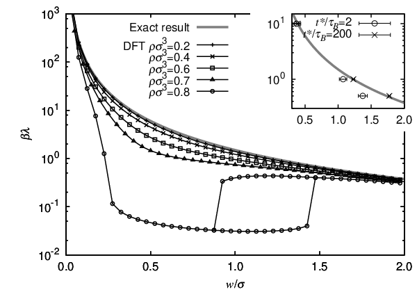
In Fig. 13 we plot the exact relationship, Eq. (62), between the strength of the confining potential, , against the width, , and compare it to the results from the equilibrium DFT approach. At the lowest densities the equilibrium DFT approach closely follows the exact result, but as the density is increased the width decreases for a given . For we find that this curve is no longer monotonic and has two disconnected branches.
Systems which are in a glassy or jammed state are by definition non-ergodic. A way of modelling non-ergodicity in Brownian dynamics is to measure the state of the system over too short a time frame. We demonstrate this effect by simulating a fluid where a single tagged particle is trapped in a parabolic potential well; c.f. Eq. (60). If the radius of the well is sufficiently large and the simulation time is too small, then the particle is not able to fully explore the outer regions of the potential well. In the inset of Fig. 13 we plot two results pertaining to this scenario where the fluid density is , and is the simulation run time. The results for the longer simulation run time agree well with the exact result, but results over the shorter time underestimate the width, particularly at the smaller values of . A similar effect may exist in the DFT approach, where the non-ergodicity arises from not including the states where the particle is far from the origin. Recall that formally the density profile from DFT is an average over all possible states of the system. Using an approximate functional some of these states may be neglected [57].
VI Concluding Remarks
On the basis of the theoretical and simulation results that we presented in this paper for the dynamics of the bulk hard sphere fluid, we conclude that the dynamical test particle limit, combined with DDFT, provides a reliable method for calculating the van Hove (and other related) dynamical pair correlation functions at low and at intermediate densities . In the previous publication [17] we have shown that the theory may be applied in a fairly straightforward manner also to inhomogeneous situations, hence we conclude that the dynamic test particle theory may indeed be used to calculate the van Hove function for fluids at interfaces and under confinement. Furthermore we have shown that, quite surprisingly, at low and intermediate densities the very simple Vineyard approximation (reviewed in Sec. II.3) is actually quantitatively fairly good. This approximation only requires as input the radial distribution function and the diffusivity and therefore provides a very useful quick approach for obtaining an approximation for the van Hove function for colloidal fluids.
The possible conclusions about the performance and even about the qualitative status of the predictions of the theory at higher densities are far more intricate though. In this regime, the theory in its current form is clearly quantitatively unreliable – compare for example, the results from BD simulations in Fig. 2(d) to those from the dynamic test particle theory shown in Fig. 3(d) for , where the theory predicts that the system jams, whereas in simulations the system is an ergodic fluid. Moreover, at even higher densities, the monodisperse hard sphere system crystallises in simulations rather than undergoing a glass transition; polydispersity would be required to suppress freezing [58]. We believe that the behaviour of the theory at higher densities can primarily be ascribed to our choice of approximation for the free energy functional – see Sec. IV.2 for the reasons for using the RY functional (53) in the present study. We believe that if we had used a more accurate functional, such as Rosenfeld’s fundamental measure theory [59, 60, 61], quantitatively more accurate results could be obtained at these higher densities. Nevertheless, the theory yields a clear prediction that there is a dynamic (glass) transition, whereby the tagged (self) particle becomes trapped in the cage formed by the surrounding particles. We can offer three possible interpretations of this result.
Firstly, one may conclude that this glass transition stems simply from the use of the approximate RY functional and since the theory predicts the glass transition to be at a density value that is well below where the glass transition is believed to occur, our results at higher densities should be disregarded.
An alternative conclusion that one may draw is that the theory is correctly describing (some of) the physics of the glass transition, but that the predictions are only qualitative in nature and occur in reality at higher densities and in polydisperse systems. Support for this point of view comes in particular from results such as those in Fig. 8, where we display results for . For , which is near to where the theory predicts the glass transition to be, we find a plateau in and the clear presence of two-stage relaxation, which indeed has been observed in hard sphere colloidal suspensions [9]. Hence our results are (qualitatively) similar to those from MCT [6, 9]. Further support for the above interpretation comes from the results in Figs. 11 and 12 for the behaviour of the free energy landscape that underlies the DDFT. The appearance of a minimum in the free energy as a function of displacement, corresponding to a particle becoming trapped in the cage formed by its neighbours, is one central prediction of the theory by Schweizer and Saltzmann [62, 63], who combined elements of MCT, DFT, and activated rate theory, in order to describe localization and transport in glassy fluids. Furthermore, given some of the work in the literature based on DFT to study the glass transition, our prediction that particles become localized should not come as a surprise: Wolynes and coworkers [64, 65, 66] developed a successful model of hard sphere vitrification, which is similar to the DFT treatment of crystallization [24, 1]. Using a random close-packed, non-periodic lattice they found a fluid-glass transition where the fluid “crystallizes” onto this lattice. The success of this method, along with its ability to model the freezing transition (onto a regular lattice), has provoked a number of further developments [67, 68, 69, 70, 71]. Other approaches [72] have investigated dense Brownian systems through modelling via certain stochastic differential equations and found that the system exhibits glassy behaviour. Thus, overall our results seem to be qualitatively consistent with other DFT based theories and with MCT for the glass transition. Nevertheless, the density where the glass transition occurs, as predicted by the theory in its present form, is far too low. Furthermore, it could be the case that the similarity between our results and those from the MCT are somehow a mathematical (rather than physical) coincidence, since an essential feature of MCT is the presence of memory in the dynamical equations. This important feature is absent from the present DDFT.
The third possible conclusion that one may draw concerns the question whether the minimum in the free energy and the localization of the tagged self particle are merely a signature of freezing in the theory. The RY functional is well-known to predict the freezing transition to occur at a density below that where it occurs in reality. It could simply be the case that this functional overly favours freezing, so that when it is applied in the way we use it here, where we constrain all density profiles, and , to be spherically symmetric, a signature of freezing shows up as the tagged self particle becoming localized.
Some merit can be found in all of the arguments outlined above and we find ourselves unable to judge which one(s) are correct. Indeed further work is required to provide a clear assessment of these issues. In particular, the dynamical test particle theory should be implemented with a more sophisticated approximation for the free energy functional than we have used here.
As we have shown, our approach is based on integrating the Smoluchowski equation (22) over all except one of the position coordinates, in order to derive an equation for the one-body density distribution. An alternative approach is to integrate over all but two of the position coordinates, in order to obtain (23) an equation for the two-body distribution function . The resulting dynamical equation depends on the three body distribution function . On making a suitable closure approximation, this provides a different starting point for studying the pair correlations in a colloidal fluid – see e.g. Refs. 52, 53 and references therein, which also consider the effect of the hydrodynamic interactions between the colloids. Developing the theory for the dynamical pair correlation functions in this way is very natural. However, we believe that the strength of our method, where we use the dynamical test particle approach allowing us to work at the one-body level, is that we are able to use DFT to close our equations and therefore we are able to describe the fluid spatial correlations very accurately.
Finally, we mention other possible directions for developing the theory in the future. One important aspect in the dynamics of colloidal dispersions, that we have entirely neglected here, are the hydrodynamic interactions between the particles. Rex and Löwen [73, 74] have shown how to include the hydrodynamic interactions in a DDFT treatment and so it would be worthwhile to use their DDFT formulation together with the present dynamical test particle limit, in order to calculate the van Hove function under the influence of hydrodynamic interactions.
A further aspect of our work, that offers possible extensions of the theory, concerns the question how to model the diffusivity of the tagged particle in a better way: In the dynamical test particle calculation one could replace the (constant) diffusion coefficient in Eq. (48) with a diffusion coefficient that depends on time; i.e. to replace . In doing this one could ensure that takes the correct values at both short and long times. However, doing this still does not treat memory effects in the dynamics. As MCT demonstrates, memory effects are key for a system to exhibit the ideal glass transition scenario[75, 9, 51]. Thus, we believe that including memory into our theory would be a crucial step in future work. This could possibly be done along the lines of the interesting work of Medina-Noyola and coworkers [12, 13, 14, 15, 16]. To include memory in our theory one could replace Eq. (29) with[16, 76, 77]:
| (66) | |||||
where the mobility coefficient has been replaced by one that is non-local in time and space. However, this would result in a considerable increase in computational complexity as within DFT the correlations in space are already treated in a complex manner and these would need to be coupled to the correlations in time. Whether such non-locality helps to cure some of the deficiencies of our approach is an open question.
Appendix A Exact Results
We consider a fluid of particles with positions , momenta and mass in the presence of an arbitrary external field that acts only on particle , . Assuming that we are in the classical limit, the Hamiltonian is given by where the contributions are due to the (classical) kinetic energy, the total inter-particle potential (not necessarily pairwise additive), and the external potential, respectively;
| (67) | |||||
| (68) | |||||
| (69) |
The canonical partition function, , is given by
| (70) |
where is Planck’s constant, and the factor results from the fact that besides particle , the remaining particles are indistinguishable. The integrations over momenta in Eq. (70) can be carried out explicitly, leaving a configuration integral over positional degrees of freedom:
| (71) |
Note that for Brownian particles is also the quantity that characterises the structure of the fluid. Substituting our external potential (69) into (71) we obtain
where in the second step we have made the substitution , for , so that we can do the integrations over the positions . This gives,
where is the configuration integral for particles where one particle is located at the origin. The Helmholtz free energy is then given by, where is the volume occupied by the particles, which yields
| (72) |
Therefore, the Helmholtz free energy only depends on the confining potential in a simple way.
One can also obtain the one body density profiles. In general, for a system of particles, the one body density profile, can be obtained from [1],
| (73) |
where the factor accounts for the indistinguishability of the particles.
For the single particle subject to the external potential we get
which is a normalised Gaussian. It can be shown that since is a Gaussian, then and are simply related by
| (74) |
and we can rewrite Eq. (72) as
| (75) |
We now seek the density profile of the remaining particles:
| (76) | |||||
To progress we make use of the formal relationship between and the two body density profile, , which for a homogeneous fluid can be shown to be [1],
where we have made the substitutions, and . Cancelling terms and rearranging we get,
| (77) |
Substituting (77) into (76) gives,
which is the normalised Gaussian convolved with .
Acknowledgements
PH thanks the EPSRC for funding under grant EP/E065619/1 and AJA gratefully acknowledges financial support from RCUK. MS and AF thank DFG for support via SFB840/A3.
References
- [1] J.-P. Hansen and I. R. McDonald, Theory of Simple Liquids (Academic Press, London, 2006), 3rd ed.
- [2] L. van Hove, Phys. Rev. 95, 249 (1954).
- [3] W. K. Kegel and A. van Blaaderen, Science 287, 290 (2000).
- [4] J.-P. Hansen and L. Verlet, Phys. Rev. 184, 151 (1969).
- [5] P. N. Pusey and W. van Megen, Nature 320, 340 (1986).
- [6] W. Götze, Liquid, Freezing and Glass Transition, Proceedings of the Les Houches Summer School, ed. J.-P. Hansen, D. Levesque, and J. Zinn-Justin (North-Holland, Amsterdam, 1989).
- [7] E. R. Weeks and D. A. Weitz, Phys. Rev. Lett. 89, 095704 (2002).
- [8] L. Berthier, G. Biroli, J.-P. Bouchaud, L. Cipelletti, D. E. Masri, D. L’Hote, F. Ladieu, and M. Pierno, Science 310, 1797 (2005).
- [9] W. van Megen and S. M. Underwood, Phys. Rev. Lett. 70, 2766 (1993).
- [10] J. M. Brader, T. Voigtmann, M. E. Cates, and M. Fuchs, Phys. Rev. Lett. 98, 058301 (2007).
- [11] J. M. Brader, M. E. Cates, and M. Fuchs, Phys. Rev. Lett. 101, 138301 (2008).
- [12] L. Yeomans-Reyna and M. Medina-Noyola, Phys. Rev. E 62, 3382 (2000).
- [13] L. Yeomans-Reyna and M. Medina-Noyola, Phys. Rev. E 64, 066114 (2001).
- [14] L. Yeomans-Reyna, H. Acuña Campa, F. Guevara-Rodríguez, and M. Medina-Noyola, Phys. Rev. E 67, 021108 (2003).
- [15] M. A. Chávez-Rojo and M. Medina-Noyola, Physica A 366, 55 (2006).
- [16] M. Medina-Noyola and P. Ramirez-Gonzalez, J. Phys.: Condens. Matter 21, 504103 (2009).
- [17] A. J. Archer, P. Hopkins, and M. Schmidt, Phys. Rev. E 75, 40501 (2007).
- [18] M. Bier, R. van Roij, M. Dijkstra, and P. van der Schoot, Phys. Rev. Lett. 101, 215901 (2008).
- [19] J. K. Percus, Phys. Rev. Lett. 8, 462 (1962).
- [20] R. Evans, Fundamentals of Inhomogeneous Fluids (New York: Dekker, 1992).
- [21] U. M. B. Marconi and P. Tarazona, J. Chem. Phys. 110, 8032 (1999).
- [22] U. M. B. Marconi and P. Tarazona, J. Phys.: Condens. Matter 12, A413 (2000).
- [23] A. J. Archer and R. Evans, J. Chem. Phys. 121, 4246 (2004).
- [24] T. V. Ramakrishnan and M. Yussouff, Phys. Rev. B 19, 2775 (1979).
- [25] G. H. Vineyard, Phys. Rev. 110, 999 (1958).
- [26] J.-P. Hansen and I. R. McDonald, Theory of Simple Liquids (Academic Press, 1986), 2nd ed., although, interestingly, the third edition [1] has this comment removed.
- [27] J. K. G. Dhont, An Introduction to Dynamics of Colloids (Elsevier, New York, 1996).
- [28] J. Dzubiella and C. N. Likos, Phys. Rev. 15, L147 (2003).
- [29] F. Penna, J. Dzubiella, and P. Tarazona, Phys. Rev. E 68, 61407 (2003).
- [30] A. J. Archer, J. Phys.: Condens. Matter 17, 1405 (2005a).
- [31] A. J. Archer, J. Phys.: Condens. Matter 17, S3253 (2005b).
- [32] M. Rex, H. Löwen, and C. N. Likos, Phys. Rev. E 72, 21404 (2005).
- [33] M. Rex, C. N. Likos, H. Löwen, and J. Dzubiella, Mol. Phys. 104, 527 (2006).
- [34] C. P. Royall, J. Dzubiella, M. Schmidt, and A. van Blaaderen, Phys. Rev. Lett. 98, 188304 (2007).
- [35] M. Rex, H. H. Wensink, and H. Löwen, Phys. Rev. E 76, 21403 (2007).
- [36] M. Rauscher, A. Dominguez, M. Krüger, and F. Penna, J. Chem. Phys. 127, 244906 (2007).
- [37] G. K. L. Chan and R. Finken, Phys. Rev. Lett. 94, 183001 (2005).
- [38] H. J. Kreuzer, Nonequilibrium Thermodynamics and its Statistical Foundations (Oxford University Press, Oxford, 1981).
- [39] P. M. Chaikin and T. C. Lubensky, Principles of Condensed Matter Physics (Cambridge University Press, Cambridge, 2000).
- [40] W. B. Russel, D. A. Saville, and W. R. Schowalter, Colloidal Dispersions (Cambridge University Press, Cambridge, 1992).
- [41] U. M. B. Marconi and P. Tarazona, J. Chem. Phys. 124, 164901 (2006).
- [42] A. J. Archer, J. Phys.: Condens. Matter 18, 5617 (2006).
- [43] U. M. B. Marconi and S. Melchionna, J. Chem. Phys. 126, 184109 (2007).
- [44] U. M. B. Marconi, P. Tarazona, F. Cecconi, and S. Melchionna, J. Phys.-Condes. Matter 20 (2008).
- [45] U. M. B. Marconi and S. Melchionna, J. Chem. Phys. 131 (2009).
- [46] A. J. Archer, J. Chem. Phys. 130, 014509 (2009).
- [47] Note that the free energy in Eq. (30) is, strictly speaking, a grand canonical quantity. This raises the issue of the validity of Eq. (30) for describing the free energy of species , which has only one particle and should strictly be treated in the microcanonical ensemble. However, if one does consider the statistical mechanics of a single particle in a trap (external potential) then one finds that one can write the ideal-gas contribution to the free energy of this particle as , i.e. differing from the expression in Eq. (30) by the term . However, due to the fact that the density profile is normalized (only one particle), then this term only contributes an additional (irrelevant) constant to the free energy (30), and this difference can be ignored. See Ref. 78 for further discussion of this issue.
- [48] M. Oettel, J. Phys.: Condens. Matter 17, 429 (2005).
- [49] P. Attard, Thermodynamics and Statistical Mechanics: Equilibrium by Entropy Maximisation (Academic Press, London, 2002).
- [50] M. P. Allen and D. J. Tildesley, Computer Simulation of Liquids (Oxford University Press, Oxford, 1987).
- [51] G. Nägele, J. Bergenholtz, and J. K. G. Dhont, J. Chem. Phys. 110, 7037 (1999).
- [52] J. F. Brady, J. Fluid Mech. 272, 109 (1994).
- [53] J. F. Brady, J. Chem. Phys. 99, 567 (1993).
- [54] D. R. Foss and J. F. Brady, J. Rheol. 44, 629 (2000).
- [55] E. R. Weeks, J. C. Crocker, A. C. Levitt, A. Schofield, and D. A. Weitz, Science 287, 627 (2000).
- [56] We have also calculated the external potentials corresponding to using the zero-dimensionality route for calculating and found that the external potentials are largely unchanged. However, in the zero dimensionality route the magnitude of the repulsion in is much smaller which results in more infilling in the core region.
- [57] D. Reguera and H. Reiss, J. Chem. Phys. 120, 2558 (2004).
- [58] S. Auer and D. Frenkel, Nature 413, 711 (2001).
- [59] Y. Rosenfeld, Phys. Rev. Lett. 63, 980 (1989).
- [60] P. Tarazona, J. A. Cuesta, and Y. Martinez-Raton, Lect. Notes Phys. 753, 247 (2008).
- [61] R. Roth, J. Phys.: Condens. Matter 22, 063102 (2010).
- [62] E. J. Saltzman and K. S. Schweizer, J. Chem. Phys. 119, 1197 (2003).
- [63] K. S. Schweizer, J. Chem. Phys. 123, 244501 (2005).
- [64] J. P. Stoessel and P. G. Wolynes, J. Chem. Phys. 80, 4502 (1984).
- [65] Y. Singh, J. P. Stoessel, and P. G. Wolynes, Phys. Rev. Lett. 54, 1059 (1985).
- [66] X. Xia and P. G. Wolynes, Phys. Rev. Lett. 86, 5526 (2001).
- [67] K. Kim and T. Munakata, Phys. Rev. E 68, 21502 (2003).
- [68] C. Kaur and S. P. Das, Phys. Rev. Lett. 86, 2062 (2001).
- [69] C. Kaur and S. P. Das, Phys. Rev. E 65, 26123 (2002).
- [70] M. Baus and J. L. Colot, J. Phys. C: Solid State Phys. 19, L135 (1986).
- [71] H. Löwen, J. Phys.: Condens. Matter 2, 8477 (1990).
- [72] L. M. Lust, O. T. Valls, and C. Dasgupta, Phys. Rev. E 48, 1787 (1993).
- [73] M. Rex and H. Löwen, Phys. Rev. Lett. 101, 148302 (2008).
- [74] M. Rex and H. Löwen, Euro. Phys. J. E 28, 139 (2009).
- [75] B. Götzelmann and S. Dietrich, Phys. Rev. E 55, 2993 (1997).
- [76] P. Ramírez-González and M. Medina-Noyola (2010), private communication.
- [77] T. Koide, G. Krein, and R. O. Ramos, Phys. Lett. B 636, 96 (2006).
- [78] A. J. Archer, Ph.D. thesis, University of Bristol (2003).