Upper Limits on Electric and Weak Dipole Moments of $W$-Boson

The existence of the electric dipole moments and weak dipole moments of elementary particles would imply $CP$ violation. Since the expected values of $CP$-odd dipole moments in the Standard Model (SM) are extremely small the measurement of significantly larger values would be evidence for physics beyond the SM.

The limits on $CP$-odd dipole moments of $W$-boson can be derived both from the analysis of high-energy experiments and from strict experimental bounds on the EDMs of other particles.

$CP$-violating triple gauge-boson couplings (TGC) $WW\gamma$ and $WWZ$ in the high-energy $e^{+}e^{-}$ collisions are investigated in Refs. [1, 2, 3, 4, 5, 6] by constructing observables sensitive to these couplings. However, one may obtain quite strict limits on the TGC parameters from the analysis of the total cross-sections only.

The most strict bounds on electric dipole moments of elementary particles are given in Table 1.

Contributions to the EDMs presented in Table 1 can originate both from the electric dipole and magnetic quadrupole moments of the $W$-boson.

The outline of the paper is as follows. In section 2 we consider $e^{+}e^{-}$ annihilation into $W^{+}W^{-}$ and obtain the bounds on the $CP$-violating TGC parameters from the analysis of the total cross-sections. In section 3 we derive upper limits on the EDM of the $W$-boson from those on the electron and neutron EDM.

We start with the consideration of the high-energy electron-positron annihilation into $W^{+}W^{-}$. In the Standard Model this reaction at the tree level is described by the Feynman graphs shown in Fig. 1.

The diagrams with the intermediate $\gamma$ and $Z$ contain three-vector-boson vertices $WW\gamma$ and $WWZ$. The general parametrization describing the vertex $WWV$ (here $V$ means $\gamma$ or $Z$) includes 14 couplings, 7 for $V=\gamma$ and 7 for $V=Z$: $g^{V}_{1}$, $\kappa_{V}$, $\lambda_{V}$, $g^{V}_{4}$, $g^{V}_{5}$, $\widetilde{\kappa}_{V}$ and $\widetilde{\lambda}_{V}$ [12, 13]. We restrict ourselves to considering only $P$-odd and $C$-even couplings, namely $\widetilde{\kappa}_{V}$ and $\widetilde{\lambda}_{V}$, because only these ones are related to the electric dipole moment $d$ and weak dipole moment (WDM) $d^{w}$ of the $W$-boson (see the corresponding Feynman graphs at the tree level in Fig. 2).

We use the following effective Lagrangian describing interaction of the $W$-boson EDM with the electromagnetic field and the WDM with the $Z$-boson field:

It should be noted that the choice of the dimension-6 operator in (1) is not unambiguous and sometimes this operator is chosen in a simpler form:

However, this discrepancy leads only to a different $q^{2}$ dependence of the form-factors. Since the energy region covered by LEP-II is not wide, one may take the form-factors to be approximately constant. Therefore, the form of the dimension-6 operator is not significant to the problem under consideration.

The $W^{-}_{\mu}(p_{-})W^{+}_{\nu}(p_{+})V_{\alpha}(q)$ vertex (see Fig. 3) corresponding to the Lagrangian (1) for on-shell $W$-bosons looks as follows [12]:

The couplings $\widetilde{\kappa}_{V}$ and $\widetilde{\lambda}_{V}$ are related to the $W$-boson EDM and WDM by [12, 14]:

$W$-bosons in the reaction $e^{+}e^{-}\to W^{+}W^{-}$ are produced in the states with the spin $S=0,2$ if the production mechanism is regular (because $CP=+1$ and $CP=(-1)^{S}$). However, if produced via the $CP$-odd vertex, $W$-bosons will be in the triplet states $S=1$ ($CP=-1$ and $CP=(-1)^{S}$). Therefore, if polarization of the particles is not taken into account the dipole moment vertices do not interfere with the regular ones, and hence their contribution to the cross-section is of second order in the dipole moments. Nevertheless the most strict limits on the dipole moments may be obtained from the analysis of the total cross-sections due to larger statistics. In this way the best restrictions on the dipole moments of $b$-quark are derived from the total cross-sections measured at LEP for $e^{+}e^{-}$ annihilation into $q\bar{q}$ [15].

We consider the reaction $e^{+}e^{-}\to W^{+}W^{-}$ in the centre-of-mass system assuming unpolarized electron and positron beams, neglecting the electron mass and summing over polarization of the final particles. Using the $WWV$ vertex parametrization (2) we obtain the following expressions for the squared matrix elements $|M|^{2}_{f^{V}_{i}}$ and the interference terms $2\mathrm{Re}\left(M^{\dagger}_{f^{V}_{6}}M_{f^{V}_{7}}\right)$ and $2\mathrm{Re}\left(M^{\dagger}_{f^{\gamma}_{i}}M_{f^{Z}_{j}}\right)$:

The functions $F_{ij}$ are as follows:

The functions $C^{V}$ and $C^{\gamma Z}$ are:

As common, we suppose hereafter the form-factors $f^{V}_{6}$ and $f^{V}_{7}$ being real [12]. We assume also local $SU(2)_{L}\times U(1)_{Y}$ gauge invariance to be preserved. It dictates [16, 17]:

So the total cross-section of the process $e^{+}e^{-}\to W^{+}W^{-}$ looks as follows:

To derive the limits, we use the LEP-II measurements of the $W$-pair production cross-section at centre-of-mass energies between 183 and 207 GeV combined by LEPEWWG [18]. The measured values and the SM predictions of $e^{+}e^{-}\to W^{+}W^{-}$ cross-sections are obtained from Table 5.1 and Table 5.2 of Ref. [18], respectively. The residuals were fitted by the second term of formula (16) with non-zero $\widetilde{\kappa}_{Z}$ and $\widetilde{\lambda}_{Z}$ assuming the relations (14, 15). The correlation matrix for the LEP combined W-pair cross-sections (Table A.2 of Ref. [18]) has been taken into account. The fit yields the 68% CL limits $|\widetilde{\kappa}_{Z}|<0.07$, $|\widetilde{\lambda}_{Z}|<0.18$ and the 95% CL limits $|\widetilde{\kappa}_{Z}|<0.13$, $|\widetilde{\lambda}_{Z}|<0.31$.

The values of $\widetilde{\kappa}_{Z}$ and $\widetilde{\lambda}_{Z}$ obtained from $e^{+}e^{-}$ annihilation are presented in Table 2. Our results obtained from the analysis of the total cross-sections are comparable with those of Refs. [5, 6] derived through analysis of the $W$ production angular distribution and distributions of the $W$ decay products.

In this section we briefly discuss the upper limits on the EDM $d_{W}$ of the $W$-boson, as derived from the strict bounds on the electron and neutron EDM [19, 20]. We follow the line of reasoning of Ref. [21] taking into account, however, the arbitrary magnetic quadrupole moment of the $W$-boson omitted in Refs [19, 20, 21].

We start the discussion with the $d_{W}$ contribution to the electron EDM. The effect is described by diagram presented in Fig. 4.

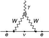
In the previous papers the EDM interaction is described by the Lagrangian

so $d_{W}=e\widetilde{\kappa}/2m_{W}$.

Then the result for the $d_{W}$ contribution to the electron EDM is

Here $\Lambda$ is the cut-off parameter for the logarithmically divergent integral over virtual momenta in the loop. Putting (perhaps, quite conservatively) $\ln(\Lambda^{2}/m_{W}^{2})\simeq 1$, one obtains with the experimental upper limit on the electron EDM [7] (see Table 1), the following bound on the dipole moment of $W$-boson:

(it corresponds to $\widetilde{\kappa}\lesssim 2\times 10^{-3}$).

However, general consideration shows that a particle of spin one can have two $P$- and $T$-odd electromagnetic moments [22]. In line with an electric dipole moment, a vector particle can have a magnetic quadrupole moment (MQM) $Q$.

Therefore, the Lagrangian contains two independent structures, corresponding to arbitrary EDM and MQM:

Now $d_{W}$ and $Q_{W}$ are related to $\widetilde{\kappa}$ and $\widetilde{\lambda}$ as follows:

and the result for the $d_{W}$ contribution to the electron EDM is

Once again putting $\ln(\Lambda^{2}/m_{W}^{2})\simeq 1$, one obtains the same bound (18, 19) on the dipole moment of $W$-boson:

Of course, this result directly depends on the cut-off parameter $\Lambda$. If one chooses $\Lambda\simeq 1$ TeV, then $\ln(\Lambda^{2}/m_{W}^{2})\simeq 5$. However, in this case one obtains the upper limit on some linear combination of $\widetilde{\kappa}$ and $\widetilde{\lambda}$, but not on the $W$-boson EDM itself.

In the case of the $W$-boson contribution to the neutron EDM considered in Ref. [21] (the EDM interaction therein is described by (17)) the same calculations, as those in the case of electron EDM, result in the following expression for the discussed contribution to the neutron dipole moment:

where $g_{0},\,h_{0}\sim 1$.

For numerical estimate one can take

so that

Then, with the result of [8] for the neutron EDM (see Table 1), one arrives at the following quite strict upper limit on the $W$-boson dipole moment:

Taking into account the second term in the Lagrangian (20) alters the contribution of $d_{W}$ to the neutron EDM:

For numerical estimate we put both expressions in curly brackets of the order of unity, so

Therefore the upper bound on the $W$-boson EDM does not change:

The contribution of $d_{W}$ to the fermion EDM (see Fig. 4) is proportional to the fermion mass. Therefore, due to the larger mass of the neutron, the limit on $d_{W}$ (31) following from $\Delta d_{n}$ is better than that (25) from $\Delta d_{e}$ by two orders of magnitude, even though the experimental upper limit on $d_{e}$ [7] is better by an order of magnitude than that on $d_{n}$ [8].

We obtained the upper limits on the $CP$-violating TGC parameters by two different methods: from the analysis of the total cross-sections of $e^{+}e^{-}\to W^{+}W^{-}$ and from strict experimental bounds on the electron and neutron EDM. There is also third way of doing this: by constructing $CP$-odd observables from the kinematic variables in the reaction $e^{+}e^{-}\to W^{+}W^{-}$. Each of these methods has its advantages and shortcomings. The analysis of the total cross-sections may give strict limits on $\widetilde{\kappa}_{V}$, $\widetilde{\lambda}_{V}$ due to high statistics and hence small statistical errors, but the bounds are obtained under the assumption that all other anomalous TGC parameters vanish, thus they are not uniquely the limits on the $CP$-violating couplings. On the contrary, $CP$-odd observables are sensitive to these couplings, but statistics is less than in the previous case. The limits derived from the bounds on the electron and neutron EDM are also uniquely the limits on $\widetilde{\kappa}_{V}$, $\widetilde{\lambda}_{V}$ and they are much better than the limits obtained from the $e^{+}e^{-}$ annihilation. However, they are of rather qualitative nature because they depend on the uncertain cut-off parameter $\Lambda$.

We are grateful to I.B. Khriplovich for many helpful discussions and suggestions as well as for critical reading of the article.

The work was supported in part by the Russian Foundation for Basic Research through Grant No. 08-02-00960-a, by the Federal Program "Personnel of Innovational Russia" through Grant No. 14.740.11.0082, and by Dmitry Zimin’s Dynasty Foundation.

References

- [1] G.J. Gounaris, C.G. Papadopoulos, Eur. Phys. J. C 2, 365 (1998).
- [2] A.A. Likhoded, G. Valencia and O.P. Yushchenko, Phys. Rev. D 57, 2974 (1998).
- [3] D. Choudhury, J. Kalinowski and A. Kulesza, Phys. Lett. B 457, 193 (1999).
- [4] M. Diehl, O. Nachtmann and F. Nagel, Eur. Phys. J. C 27, 375 (2003); Eur. Phys. J. C 32, 17 (2003).
- [5] The OPAL Collaboration, Eur. Phys. J. C 19, 229 (2001).
- [6] DELPHI Collaboration, Eur. Phys. J. C 54, 345 (2008).
- [7] B.C. Regan, E.D. Commins, C.J. Schmidt, D. DeMille, Phys. Rev. Lett. 88, 071805 (2002).
- [8] C.A. Baker et al., Phys. Rev. Lett. 97, 131801 (2006).
- [9] V.F. Dmitriev, R.A. Sen’kov, Phys. Rev. Lett. 91, 212303 (2003).
- [10] W.C. Griffith, M.D. Swallows, T.H. Loftus, M.V. Romalis, B.R. Heckel, E.N. Fortson, Phys. Rev. Lett. 102, 101601 (2009).
- [11] G.W. Bennett et al., Phys. Rev. D 80, 052008 (2009).
- [12] K. Hagiwara, R.D. Peccei, D. Zeppenfeld, K. Hikasa, Nucl. Phys. B 282, 253 (1987).
- [13] G. Gounaris et al., CERN 96-01, 525, arXiv:hep-ph/9601233.
- [14] A. Queijeiro, Phys. Rev. D 39, 3507 (1989).
- [15] A.E. Blinov, A.S. Rudenko, Nucl. Phys. B (Proc. Suppl.) 189, 257 (2009).
- [16] M.S. Bilenky, J.L. Kneur, F.M. Renard, D. Schildknecht, Nucl. Phys. B 409, 22 (1993).
- [17] K. Hagiwara, J. Woodside, D. Zeppenfeld, Phys. Rev. D 41, 2113 (1990).
- [18] LEPEWWG group, hep-ex/0612034.
- [19] F. Salzman, G. Salzman, Phys. Lett. 15, 91 (1965); Nuovo Cimento A 41, 443 (1966).
- [20] F.J. Marciano, A. Queijeiro, Phys. Rev. D 33, 3449 (1986).
- [21] A.G. Grozin, I.B. Khriplovich, A.S. Rudenko, Nucl. Phys. B 821, 285 (2009).
- [22] I.Yu. Kobzarev, L.B. Okun’, M.V. Terentyev, Sov. Phys. JETP Lett. 2, 289 (1965).