Measurement-induced quantum entanglement recovery
Abstract
By using photon pairs created in parametric down conversion, we report on an experiment, which demonstrates that measurement can recover the quantum entanglement of two qubit system in a pure dephasing environment. The concurrence of the final state with and without measurement are compared and analyzed. Furthermore, we verify that recovered states can still violate Bell’s inequality, that is, to say, such recovered states exhibit nonlocality. In the context of quantum entanglement, sudden death and rebirth provide clear evidence, which verifies that entanglement dynamics of the system is sensitive not only to its environment, but also on its initial state.
pacs
03.67.Mn, 03.65.Ud, 03.65.YzQuantum entanglement, as a unique feature without a classical counterpart of many-body system, has been instrumental in studying fundamental aspects of quantum physics [1] as well as being central in practical applications in the areas of quantum computation and quantum cryptography [2, 3, 4, 5]. Today, sources of entangled states can be prepared in various kinds of physical systems [6]. Entanglement, even within multi-particle and multi-dimensional systems [7, 8], can be implemented, although, these are flimsy and are subject to unavoidable degradation, which is caused by interactions with their environments [9, 10]. To have any practical value in quantum computation and communication, long distance nonlocality and extended coherence storage and rebirth [11] of entangled states have become important focal points of research around the world. The key issue behind solving these problems is in determining the dynamical behavior of entanglement within the system’s environment, something, which to date, has not been well understood. Commendably, a factorization law, which describes the entanglement dynamics under a one-side noisy channel has recently been proposed [12] and has subsequently been verified in two independent experiments [13]. Moreover, it has been discovered that entanglement evolution is not only related to environmental factors but is also sensitive to its initial state [14, 15].
Quantum measurement, that feature, which distinguishes the quantum from the classical regimes [17], is often interpreted within the orthogonal projection model given by Von Neumann [18], but has been reexpressed in the past 30 years or so, more and more within the framework of quantum decoherence theory [19] (for reviews see [9, 17]). In that setting, a complete quantum measurement is divided into two stages: The first stage corresponds to the entanglement of the information-carrying qubit of the measured quantum system with the record bit of the measurement apparatus; the second stage corresponds to the decoherence of the detector-system combination, which occurs in an uncontrollable environment [17]. The latter will covert the density matrix that describes the combination into diagonal form, which physically represents the spreadings of the quantum information contained in the combined system into the uncontrollable environment and essentially turns the quantum measurement into a classical one. Because of the uncontrollability and unavoidability of environment-induced decoherence that features prominently in this second stage, it is impossible to recover quantum information once the quantum measurement has been completed. For example, if a conventional experiment to measure the polarization of a single photon has completed, to retrieve that qubit of quantum information is as difficult as extracting it from the single photon detector and the observer’s brain. Fortunately, quantum measurement need not be so catastrophic and can be implemented step by step, even partially [20]. It has been pointed out that, within the first stage of quantum measurement, recovery can be brought about by the coherence of a single qubit that has dissipated into a non-Markovian environment [21].
On the basis of this work by Xu et al Xu we experimentally prove that subsequent quantum measurement, which erases [16] the path information introduced in the previous measurement can recover the entanglement that has been degraded in a non-Markovian environment and that even rebirth of entanglement after entanglement sudden death (ESD) [11] can be effected. In this paper, we describe how we can change the entanglement evolution by using some specified operations on the state before or during the interaction, more precisely, two sequential measurements can recover the entanglement and, further more, preserve it.
The experimental setup is shown schematically in Figure 1. Two 0.5 mm thick beta-barium-borate (BBO) crystals, cut at 29.18∘ for type-I phase matching and aligned so their optical axes are perpendicular to each other, are pumped by using focused ultraviolet (UV) pulses polarized at 45∘, which are frequency doubled from a Ti:sapphire laser with the center wavelength mode locked at 800 nm (with 130 fs pulse width and a 76 MHz repetition rate). Degenerate polarization-entangled photon pairs at 800 nm are generated by spontaneous parametric down conversion (SPDC) at a 3∘ angle with the pump beam [22]. By compensating the time difference between - and -polarized components with birefringent elements (LiNbO3 and YVO4), one of the maximal polarization-entangled states, the well-known Bell state [30], can be produced with high fidelity. This initial state can be mathematically written as
| (1) |
where H and V represent the horizontal and vertical polarizations, respectively, while the two elements in the Dirac ket label the photons states, the left in path and the right in path .
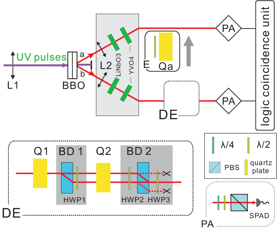
Decoherence due to the environment is simulated by controllable birefringent elements, which can couple the photon’s frequency with its polarization [23, 24]. In our experiment, we use quartz plates Q1 with thickness and Q2 with thickness , to simulate this decoherence aspect. The optical axes of the plates are both horizontally set.
At the beginning, we consider the evolution of the state given by equation (1) in such an environment, which assume, for simplicity, that the photon’s frequency distribution is a function. The final state of the two photons after the photon in mode passes through Q1 and Q2 takes the following form
| (2) |
where the parameter is proportional to and represents the frequency of the photon in path . In our experiment, where is the velocity of light in vacuo and represents the difference between refractive indices of ordinary and extraordinary light. Therefore, a deterministic relative phase is introduced between and for a single frequency, which differs for different frequencies. According to the decoherence mode [23, 24], the environment is actually composed of a photon’s frequencies that are coupled to the information carriers (viz. polarization of photons) by means of birefringent elements. For photons with a frequency distribution , the overall state should equal the integral over the frequency distribution, which forms a less correlated state, which essentially destroys the coherence of the qubits [23]. Therefore, the final state in Eq. (2) should be replaced by the following reduced density operator [24]
| (3) |
where the photon’s frequency distribution in path is normalized as and the nondiagonal coefficient represents the decoherence parameter.
Actually, for a decoherence environment composed of photon’s frequency, the decoherence parameter is related to the frequency distribution function. In our experiment, this is taken to be a Gaussian function, that is, , which is determined by the interference filters (IF) placed in front of the single photon detectors. The parameter is the central frequency, and is the bandwidth. By working out the integral, we obtain .
For a quantitative analysis of the entanglement evolution in the experiment, a parameter, which represents the degree of entanglement, should be introduced. The concurrence [26], which is widely used in studying two qubit states, is defined as
| (4) |
where is the density matrix of a two-qubit state in the canonical basis ; are the eigenvalues in decreasing order of the Hermitian matrix with , which corresponds to the complex conjugate of . According to Eq. (3), for an initial Bell state input, we obtain . Thus, concurrence degrades exponentially and approaches zero as Q1 and Q2 become thicker, which means the final state, after sufficient interaction time, evolves into the maximally mixed state without any remaining entanglement [solid line in Fig. 2(A)]. However, for some other frequency distribution, some unusual phenomena will arise, for example, entanglement collapse and revival [25].
Then, we consider the case with a measurement apparatus (M), which comprises two beam displacing prisms (BD1 and BD2) with horizontally-set optical axes, half-wave plate 1 (HWP1) with optical axes set at 22.5∘, which implements the Hadamard operation, HWP2 with optical axes set at -22.5∘, which implements (where,, ), and HWP3 with perpendicularly set optical axes to implement the bit-flip operation. BD1 measures photon’s polarization in H/V basis and introduces the path information as a probe bit. Before this measurement is completed, the second decoherence environment is inserted, and then, the path information is erased by BD2, which realizes a postselection of the recovered state. The output state after passing through Q1, BD1, HWP1 and Q2, can be written as
| (5) |
where and , subscripts I and II denote the upper and lower paths between the two BDs, respectively. By subsequently erasing path information introduced in the previous measuring operation by HWP2, BD2 and HWP3, we obtain the final state represented as
| (6) |
Similar to the above treatment, the reduced density matrix of this final state is written as
| (7) |
where
According to Eq. (4), the concurrence is . From the complicated form of , here, the entanglement evolution is not as simple as that in the previous case, and it sensitive to the phase. Numerical analysis shows there will be entanglement recovery with increases in , as remains fixed. The concurrence oscillates if is sufficiently thin, while the amplitude narrows to zero if is thick enough. Because the maximal recovery point lies within the envelope composed of the integral and the zero point of the phase is extremely hard to determine, here, we only consider the integral length of the quartz plates [solid line in Fig. 2(B) and Fig. 2(C)]. Although this is sufficient for studying entanglement recovery, under this consideration, the probability of success decreases exponentially from 1 to 0.5. More significantly, the entanglement of the final state will remain unchanged with increasing when is large enough, and no matter how thick is, that is, to say, no matter how less entanglement remains, the entanglement between two particles can be recovered to a maximal expectation value 0.5 at .
In fact, the dynamics of entanglement in bipartite quantum systems not only is sensitive to their environment, but also is sensitive to their initial state [14, 15]. In Ref [25], entanglement collapse and revival occur when the input biphoton is prepared in the form of a Werner state [28] with a spectrum discretized within a Gaussian envelope. There will be no entanglement revival if the spectrum takes the Gaussian form in that experiment. However, a revival of the same initial state with a Gaussian spectrum can occur by inserting M in this experiment. This is explained as follows.
Applying a Hadamard operation on the photon state in mode of the maximal entangled state and by allowing it to pass though a dephasing environment at bases, we get the state
| (8) |
By integrating over all frequencies of the photon in mode , the partially entangled input state can be mathematically expressed in the following density matrix
| (9) |
where is the decoherence parameter in path . The photon in mode then passes through the decoherence environment with a measuring apparatus; the final state in the single frequency case can be written as
| (10) |
The band width of the interference filters used in our experiment is so narrow that we can integrate over the frequencies of the photon in mode and separately [29]. Therefore, if the photon frequencies are considered to have Gaussian distribution profiles, the density matrix of the final state is written as
| (11) |
According to Eq. (4), we obtain a concurrence of . For nonnegative with different , entanglement, sudden death and re-birth will occur if the decoherence time in Q1 and Q2 are changed [solid line in Fig. 2(D) with just integral lengths of quartz plates]. No matter how thick Q1 is, entanglement between the two particles is found to indicate a full rebirth to an identical maximal value at . That is, to say, full recovery with analogous levels can be achieved regardless of the time duration taken for the ESD.


The experimental results are shown in Fig. 2. The characteristics of the IFs used before the single photon detectors are of bandwidth 3 nm and coatings at 800 nm. We can treat for small frequency distributions. The maximally entangled state is prepared with a concurrence of 0.962 0.029. In Fig. 2(a), the concurrence degrades exponentially and gradually tends to zero, which obeys the half-life law. Because there is no phase sensitivity, experimental results (dots) agreed well with theory within the error range. In Fig. 2(b), M is inserted at the point where the concurrence is 0.262 0.024. The maximally recovered concurrence in the experiment is 0.609 0.026 at , and the concurrence is unchanged within the error range when exceeds 683. In Fig. 2(c), the point at which M is inserted is where the concurrence tends to zero, that is, to say, there are few entanglement at this point. Incidentally, the maximally recovered entanglement measured in the experiment is 0.518 0.025 at about , which agrees well with theoretical predictions. In Fig. 2(d), the partially entangled input state with concurrence 0.704 0.019 is prepared by inserting an HWP with optical axes set at 22.5∘ and quartz plates of thickness 98 with horizontally-set optical axes in mode a. We insert M at at which ESD has occurred, and there is no entanglement; entanglement rebirth occurs at about and then the entanglement collapses at about again. The concurrence is corrected to zero according to Eq. (4) when its measured value is negative. Entanglement can be reborn at a maximal value 0.276 0.013 in the experiment.
Nonlocality, as a particular characteristic of quantum mechanics, has changed the viewpoint and methods in understanding nature at its fundamental level. Since it can be studied by the well known Bell inequality [30], a quantum state with nonlocal correlations could be a very useful feature to exploit in future quantum technologies [31]. In our experiment, the maximally recovered entangled state in Fig. 2(b) and Fig. 2(c) can be proven to be nonlocal by the more convenient Clauser-Horne-Shimony-Holt (CHSH) inequality [32], for any local realistic theory, where
| (12) |
with
Here, represent the linear polarization setting in path a and path b separately and . By calculating the maximal value of S from the measured density matrix of the maximally recovered state, we get in Fig. 2(B) and in Fig. 2(C). Accordingly, the measured values of S are 2.336 0.003 and 2.210 0.003, which violate the local realism limit 2 by over 104 and 64 standard deviations, respectively.
The extraordinary phenomenon of entanglement recovery induced by a measurement, can be understood in the quantum framework of a partial measurement and reversal [20]. BD1 measures the photon’s polarization in H/V basis. Partial measurement in H/V basis in the upper path and a reversal operation with the same strength [33] in the lower path is implemented by BD2. The photons in the two dark ports of BD2 are abandoned, this can be considered as a non-response of the detector to the coincidence detection. Because partial measurement and reversal with the same intensity can restore the initial entanglement [20] and the phase difference introduced by only changes the strength, we believe that entanglement is preserved with the increasing while the recovery is an optical spin-echo effect introduced by HWP1.
To summarize, we have report on an experiment, which shows that entanglement can be recovered by a process of measurement followed by quantum eraser in a non-Markovian environment. Simultaneously, the maximally recovered states can be verified to violate the CHSH inequality with high standard deviations, which confirms theirs quantum character. This result can be used to eliminate the influence of dephasing. Another encouraging aspect is that, even if the state has been thoroughly disentangled, that is, to say, ESD has occurred, the entanglement can still be revived from non-Markovian environments regardless of decoherence time durations. This can be used to implement controllable recovery of entanglement. Entanglement dynamics considering other coding and decoding protocol can be studied in future work.
This work was supported by National Fundamental Research Program and the National Natural Science Foundation of China (Grant No.60621064 and 10874162).
References
- [1] A. Zeilinger, Rev. Mod. Phys. 71, S288 (1999).
- [2] M. A. Nielsen and I. L. Chuang, Quantum Computation and Quantum Information (Cam- bridge University Press, Cambridge, England, 2000).
- [3] R. Raussendorf, H. J. Briegel, Phys. Rev. Lett. 86, 5188 (2001).
- [4] J. L. O’Brien, Science 318, 1567 (2007).
- [5] A. K. Ekert, Phys. Rev. Lett. 67, 661 (1991).
- [6] T. D. Ladd, F. Jelezko, R. Laflamme, Y. Nakamura, C. Monroe and J. L. O’Brien, Nature 464, 45 (2010).
- [7] A. Rossi, G. Vallone, F. De Martini, and P. Mataloni, Phys. Rev. A 78, 012345 (2008).
- [8] C. Y. Lu, X. Q. Zhou, O. Gühne, W. B. Gao, J. Zhang, Z. S. Yuan, A. Goebel, T. Yang, and J. W. Pan, Nature Phys. 3, 91 (2007).
- [9] W. H. Zurek, Rev. Mod. Phys. 75, 715 (2003).
- [10] F. Mintert, A. R. R. Carvalho, M. Kus, A. Buchleitner, Phys. Rep. 415, 207 (2005).
- [11] T. Yu and J. H. Eberly, Science 323, 598 (2009).
- [12] T. Konrad, F, de Melo, M. Tiersch, C. Kasztelan, A. Aragão, and A. Buchleitner, Nature Phys. 4, 99 (2008).
- [13] O. Jiménez Farías, C. Lombard Latune, S. P. W alborn, L. Davidovich, P. H. S. Ribeiro, Science 324, 1414 (2009); J. S. Xu, C. F. Li, X. Y. Xu, C. H. Shi, X. B. Zou and G. C. Guo, Phys. Rev. Lett. 103, 240502 (2009).
- [14] K. Roszak and P. Machnikowski, Phys. Rev. A 73, 022313 (2006).
- [15] T. Yu and J. H. Eberly, Phys. Rev. Lett. 97, 140403 (2006).
- [16] M. O. Scully, B. G. Englert and H. Walther, Nature 351, 111 (1991).
- [17] W. H. Zurek, Physics Today 44, 36 (1991).
- [18] Von Neumann J, Mathematical Foundations of Quantum Mechanics (Princeton, NJ:Princeton University Press) (1955)
- [19] W. H. Zurek, Phys. Rev. D 24, 1516 (1981); ibid. 26, 1862 (1982).
- [20] A. C. Elitzur, S. Dolev, Phys. Rev. A 63, 062109 (2001).
- [21] J. S. Xu, C. F. Li, M. Gong, X. B. Zou, L. Chen, G. Chen, J. S. Tang and G. C. Guo, New J. Phys. 11, 043010 (2009).
- [22] P. G. Kwiat, E. Waks, A. G. White, I. Appelbaum, and P. H. Eberhard, Phys. Rev. A 60, R773 (1999).
- [23] P. G. Kwiat, A. J. Berglund, J. B. Altepeter and A. G. White, Science 290, 498 (2000).
- [24] A. J. Berglund, arXiv:quant-ph/0010001 (2000).
- [25] J. S. Xu, C. F. Li, M. Gong, X. B. Zou, C. H. Shi, G. Chen, and G. C. Guo, Phys. Rev. Lett. 104, 100502 (2010).
- [26] W. K. Wootters, Phys. Rev. Lett. 80, 2245 (1998).
- [27] D. F. V. James, P. G. Kwiat, W. J. Munro, and A. G. White, Phys. Rev. A 64, 052312 (2001).
- [28] R. F. Werner, Phys. Rev. A 40, 4277 (1989).
- [29] Z. Y. Ou, J. -K. Rhee and L. J. Wang, Phys. Rev. A 60, 593 (1999).
- [30] J. S. Bell, Physics 1, 195 (1964); Rev. Mod. Phys. 38, 447 (1966).
- [31] N. Gisin, Science 326, 1357 (2009).
- [32] J. F. Clauser, M. A. Horne, A. Shimony and R. A. Holt, Phys. Rev. Lett. 23, 880 (1969).
- [33] The stength will attenuate from 1 to 0.5 with increasing while keeping the equivalence between partial measurement and erasure.