Monte Carlo treatment of hadronic interactions in enhanced Pomeron scheme: I. QGSJET-II model

Nowadays Monte Carlo (MC) generators of hadronic interactions are standard tools for data analysis in high energy collider and cosmic ray (CR) fields. The idea behind employing such MC models is twofold. First of all, they provide a bridge between rigorous theoretical approaches and corresponding experimental studies, thus allowing to confront novel ideas against observations. On the other hand, MC simulations are an inevitable part of contemporary experimental analysis procedures, a measurement of new phenomena depending crucially on the understanding of the corresponding detector response and of the contribution of the “standard” hadronic physics which is mimicked with the help of the MC tools.

In particular, hadronic interaction models play an important role in investigations of very high energy cosmic rays. Because of the extremely low flux of such ultra-energetic particles, they can not be detected directly. Instead one infers their properties from measured characteristics of nuclear-electro-magnetic cascades, so-called extensive air showers (EAS), induced by them in the atmosphere. The corresponding analysis relies crucially on the MC treatment of the cascade development, most importantly, of its backbone - the cascade of hadron-nucleus (nucleus-nucleus) interactions in the atmosphere. The peculiarity of cosmic ray applications of hadronic interaction generators is related to the fact that one has to treat hadronic collisions at energies orders of magnitude higher than ones of present day colliders and that EAS characteristics depend strongly on model predictions for very forward spectra of secondary particles. As a consequence, CR interaction models, like DPMJET [1], EPOS [2], QGSJET [3], or SYBILL [4], which are designed to treat general inelastic hadronic collisions, are developed in the framework of the Reggeon Field Theory (RFT) [5], which allows one to take into consideration contributions from both “soft” and “hard” parton dynamics to the interaction mechanism.

Soft nonperturbative interactions are described as soft Pomeron exchanges and dominate hadronic collisions at large impact parameters, thus giving important contributions to total, inelastic, and diffractive hadron-nucleus (nucleus-nucleus) cross sections. On the other hand, at sufficiently high energies the role of so-called semihard hadronic collisions which involve partons of moderately large virtualities is significantly enhanced, the smallness of the corresponding strong coupling being compensated by large collinear and infra-red logarithms and by high density of small $x$ partons. A convenient way to include such processes in the RFT treatment is provided by the “semihard Pomeron” approach [6, 7] where the perturbative part of an “elementary” semihard rescattering is described within the DGLAP formalism, which is preceded by nonperturbative parton cascades (“soft preevolution”) described as soft Pomeron emissions.

Additionally, high parton densities reached in “central” collisions of hadrons and, especially, nuclei result in significant nonlinear corrections to the interaction dynamics, related to parton shadowing and saturation [8]. In MC generators, such effects are typically accounted for in a phenomenological way, via energy-dependent parametrizations of some model parameters. The drawback of such constructions is evident: with nonlinear effects dominating the interaction mechanism in the very high energy limit, model predictions are governed by the choice of the corresponding empirical parametrization, rather than by the underlying theoretical approach.

In this work, we choose an alternative way, treating nonlinear interaction effects in the RFT framework as Pomeron-Pomeron interactions [9, 10, 11], based on the recent progress in the resummation of the corresponding, so-called enhanced, RFT diagrams [12, 13, 14]. A MC implementation of such an approach has been hampered for a long time by two factors. First, with the energy increasing, enhanced graphs of more and more complicated topologies start to contribute significantly to the scattering amplitude and to partial cross sections for particular hadronic final states. Thus, dealing with enhanced diagrams, all-order resummation of the corresponding contributions is a must, both for elastic scattering diagrams and for the cut diagrams representing particular inelastic processes. Secondly, it is quite nontrivial to split the complete set of cut enhanced diagrams into separate classes characterized by positively-defined contributions which could be interpreted probabilistically and employed in a MC simulation procedure. While the first problem has been addressed in [12, 13, 14], the MC implementation of the approach is discussed in the present work. Here we mainly address the construction of the model while the results for various particle production processes and applications of the model for calculations of EAS development will be the subject of the forthcoming publication [15].

The outline of the paper is as follows. In Section 2, the calculation of hadron-hadron scattering amplitude is discussed, taking into account enhanced diagram contributions. In Section 3, we consider unitarity cuts of elastic scattering diagrams and define partial contributions for various “macro-configurations” of the interaction, which are employed in the corresponding MC procedure, as described in Section 4. Finally, in Section 5, we discuss characteristic features of the developed model, calibration of model parameters, and present the model results for various hadronic cross sections.

In the RFT approach, high energy hadron-hadron scattering amplitude is defined by multiple scattering graphs of the kind depicted in Fig. 1.

The elementary rescattering contributions correspond to independent parton cascades developing between the projectile and target hadrons, which are described by Pomeron exchanges, and to parton cascades which strongly overlap in the phase space and interact with each other, which is described as Pomeron-Pomeron interactions. Thus, applying the multichannel (Good-Walker-like) eikonal scheme [16, 17] to account for contributions of small mass intermediate states between Pomeron emissions, elastic hadron $a$ - hadron $d$ scattering amplitude is defined as [13]

	$\displaystyle f_{ad}(s,b)=i\,\sum_{j,k}C_{j/a}C_{k/d}\,\left[1-e^{-\frac{1}{2}\Omega_{ad(jk)}(s,b)}\right]$		(1)
	$\displaystyle\Omega_{ad(jk)}(s,b)=2\chi_{ad(jk)}^{\mathbb{P}}(s,b)+2\chi_{ad(jk)}^{{\rm enh}}(s,b)\,.$		(2)

Here $s$ and $b$ are c.m. energy squared and impact parameter for the interaction, $C_{j/a}$ defines partial weight for hadron $a$ elastic scattering eigenstate $|j\rangle$ ($|a\rangle=\sum_{j}\sqrt{C_{j/a}}|j\rangle$, $\sum_{j}C_{j/a}=1$), $\chi_{ad(jk)}^{\mathbb{P}}$ and $\chi_{ad(jk)}^{{\rm enh}}$ are eikonals corresponding to an exchange of a Pomeron or of an irreducible enhanced (Pomeron-Pomeron interaction) graph between the projectile and target hadrons, the latter being represented by eigenstates $|j\rangle$ and $|k\rangle$.

In this work, we use the “semihard Pomeron” approach [6, 7] to account for contributions of both nonperturbative soft processes and of “semihard” ones, the latter corresponding to parton cascades which develop at least partly in the perturbative region of relatively high virtualities $|q^{2}|>Q_{0}^{2}$, $Q_{0}^{2}$ being some cutoff for pQCD being applicable. Describing the former as phenomenological soft Pomerons and the latter by “semihard Pomeron” exchanges, the “general Pomeron” eikonal is given by the sum of the two contributions:

$$\chi_{ad(jk)}^{\mathbb{P}}(s,b)=\chi_{ad(jk)}^{\mathbb{P}_{{\rm soft}}}(s,b)+\chi_{ad(jk)}^{\mathbb{P}_{{\rm sh}}}(s,b)\,.$$

(3)

The soft Pomeron eikonal $\chi_{ad(jk)}^{\mathbb{P}_{{\rm soft}}}$ is expressed via Pomeron emission vertices $N^{\mathbb{P}}$ and the Pomeron propagator $D^{\mathbb{P}}$ as

$$\chi_{ad(jk)}^{\mathbb{P}_{{\rm soft}}}(s,b)=\frac{1}{8\pi^{2}\,i\,s}\>\int\!d^{2}q\;e^{-i\,\vec{q}\,\vec{b}}\,\int\!dx_{1}\,dx_{2}\;N_{j/a}^{\mathbb{P}}(x_{1},q^{2})\,N_{k/d}^{\mathbb{P}}(x_{2},q^{2})\,D^{\mathbb{P}}(x_{1}x_{2}s,q^{2})\,,$$

(4)

where

$$D^{\mathbb{P}}(\hat{s},t)=8\pi\,i\,s_{0}\,(\hat{s}/s_{0})^{\alpha_{\mathbb{P}}}\>e^{\alpha^{\prime}_{\mathbb{P}}\,\ln(s/s_{0})\>t},$$

(5)

with $\alpha_{\mathbb{P}}$ and $\alpha^{\prime}_{\mathbb{P}}$ being the intercept and the slope of the Pomeron Regge trajectory and $s_{0}\simeq 1\;{\rm GeV}^{2}$ - the hadronic mass scale.

The Pomeron emission vertices are parametrized as

$$N_{j/a}^{\mathbb{P}}(x,t)=\gamma_{j/a}\,e^{\Lambda_{j/a}\,t}\,x^{-\alpha_{{\rm part}}}\,(1-x)^{\alpha_{{\rm lead}}},$$

(6)

where the exponents $\alpha_{{\rm part}}\simeq 0$ and $\alpha_{{\rm lead}}$ are related to intercepts of secondary Regge trajectories [18, 7].

The semihard contribution $\chi_{ad(jk)}^{\mathbb{P}_{{\rm sh}}}$ corresponds to a piece of QCD parton ladder sandwiched between two soft Pomerons (see Fig. 2)

and is defined as [7, 19]

	$\displaystyle\chi_{ad(jk)}^{\mathbb{P}_{{\rm sh}}}(s,b)=\frac{1}{32\pi^{2}s_{0}^{2}}\>\int\!d^{2}q\;e^{-i\,\vec{q}\,\vec{b}}\,\int\!dx_{1}\,dx_{2}\;N_{j/a}^{\mathbb{P}}(x_{1},q^{2})\,N_{k/d}^{\mathbb{P}}(x_{2},q^{2})\,\int\!dx^{+}\,dx^{-}$
	$\displaystyle\times\>\mathfrak{Im}D^{\mathbb{P}}(s_{0}/x^{+},q^{2})\;\mathfrak{Im}D^{\mathbb{P}}(s_{0}/x^{-},q^{2})\sum_{I,J=g,q_{s}}g_{I}(x^{+})\;g_{J}(x^{-})\;\sigma_{IJ}^{{\rm QCD}}(x^{+}x^{-}x_{1}x_{2}s,Q_{0}^{2})\,,$		(7)

where the vertices $g_{I}$ for parton $I$ (gluon or sea quark)¹¹ 1 For brevity, we do not discuss explicitly valence quark contributions to the semihard eikonal; the corresponding description can be found elsewhere [7, 19]. coupling to the soft Pomeron are parametrized as

	$\displaystyle g_{g}(z)=r_{g}\,(1-w_{qg})\,(1-z)^{\beta_{g}}$
	$\displaystyle g_{q_{s}}(z)=r_{g}\,w_{qg}\,\int_{z}^{1}\!dy\;y^{\alpha_{\mathbb{P}}-1}\>P_{qg}(y)\>(1-z/y)^{\beta_{g}},$		(8)

with $P_{qg}(y)$ being the Altarelli-Parisi splitting function and the constant $r_{g}$ being fixed by momentum conservation for parton distribution functions (PDFs).

The contribution $\sigma_{IJ}^{{\rm QCD}}(x^{+}x^{-}s,Q_{0}^{2})$ of parton ladder with the virtuality cutoff $Q_{0}^{2}$ and with the leg-parton types $I$, $J$ and light cone momentum fractions $x^{+}$, $x^{-}$ is defined in a standard way (see, e.g. [7, 19])

	$\displaystyle\sigma_{IJ}^{{\rm QCD}}(\hat{s},Q_{0}^{2})=K\sum_{I^{\prime},J^{\prime}}\int\!dz^{+}\,dz^{-}\int dp_{t}^{2}\;E_{I\rightarrow I^{\prime}}^{{\rm QCD}}(z^{+},Q_{0}^{2},M_{{\rm F}}^{2})\>E_{J\rightarrow J^{\prime}}^{{\rm QCD}}(z^{-},Q_{0}^{2},M_{{\rm F}}^{2})$
	$\displaystyle\times\frac{d\sigma_{I^{\prime}J^{\prime}}^{2\rightarrow 2}(z^{+}z^{-}\hat{s},p_{t}^{2})}{dp_{t}^{2}}\>\Theta(M_{{\rm F}}^{2}-Q_{0}^{2})\,,$		(9)

with $d\sigma_{IJ}^{2\rightarrow 2}/dp_{t}^{2}$ being the differential parton-parton cross section, $p_{t}$ - parton transverse momentum in the hard process, $M_{{\rm F}}^{2}$ - the factorization scale (here $M_{{\rm F}}^{2}=p_{t}^{2}/4$), and with $E_{I\rightarrow I^{\prime}}^{{\rm QCD}}(z,Q_{0}^{2},Q^{2})$ describing the evolution of the parton density from the virtuality scale $Q_{0}^{2}$ to $Q^{2}$. The factor $K\simeq 1.5$ is designed to take effectively into account higher order QCD corrections.

The idea behind Eq. (7) is to split parton evolution in an elementary scattering process in two parts: i) nonperturbative soft one described phenomenologically by the soft Pomeron asymptotics; ii) parton cascading at $|q^{2}|>Q_{0}^{2}$, treated within the DGLAP formalism. The former is characterized by a significant parton diffusion in the transverse plane and, in the absence of nonlinear corrections, forms parton (sea quark or gluon) momentum and impact parameter distributions at the virtuality scale $Q_{0}^{2}$ [7, 19, 20]. During the latter, parton transverse displacements can be neglected, leaving only the momentum-dependent part, Eq. (9), which is characterized by a stronger energy-rise compared to the soft Pomeron amplitude and drives therefore the high energy behavior of the semihard contribution (7).

To calculate enhanced diagram contributions, we adopt multi-Pomeron vertices of the form [11]

$$G^{(m,n)}=G\,\gamma_{\mathbb{P}}^{m+n},$$

(10)

where $m$ and $n$ are numbers of Pomerons connected to the vertex from the projectile, respectively target, side ($m+n\geq 3$) and the constant $G$ is related to the triple-Pomeron coupling $r_{3\mathbb{P}}$ as $G=r_{3\mathbb{P}}/(4\pi\gamma_{\mathbb{P}}^{3})$.

The eikonal $\chi_{a(j)}^{\mathbb{P}}(y,b)$ for a “general Pomeron” exchange between hadron $a$ (represented by eigenstate $|j\rangle)$ and a multi-Pomeron vertex, the two being separated from each other by rapidity $y$ and transverse distance $b$, also receives contributions from both soft and semihard processes

$$\chi_{a(j)}^{\mathbb{P}}(y,b)=\chi_{a(j)}^{\mathbb{P}_{{\rm soft}}}(y,b)+\chi_{a(j)}^{\mathbb{P}_{{\rm sh}}}(y,b)\,,$$

(11)

with the partial contributions $\chi_{a(j)}^{\mathbb{P}_{{\rm soft}}}$ and $\chi_{a(j)}^{\mathbb{P}_{{\rm sh}}}$ being defined similarly to (4), (7) [20]:

	$\displaystyle\chi_{a(j)}^{\mathbb{P}_{{\rm soft}}}(y,b)=\frac{\gamma_{\mathbb{P}}}{8\pi^{2}\,i\,s_{0}\,e^{y}}\>\int\!d^{2}q\;e^{-i\,\vec{q}\,\vec{b}}\,\int\!dx_{1}\;N_{j/a}^{\mathbb{P}}(x_{1},q^{2})\,D^{\mathbb{P}}(x_{1}s_{0}\,e^{y},q^{2})$		(12)
	$\displaystyle\chi_{a(j)}^{\mathbb{P}_{{\rm sh}}}(y,b)=\frac{\gamma_{\mathbb{P}}}{32\pi^{2}s_{0}^{2}}\>\int\!d^{2}q\;e^{-i\,\vec{q}\,\vec{b}}\,\int\!dx_{1}\;N_{j/a}^{\mathbb{P}}(x_{1},q^{2})\,\int\!dx^{+}\,dx^{-}\>\mathfrak{Im}D^{\mathbb{P}}(s_{0}/x^{+},q^{2})$
	$\displaystyle\times\;\mathfrak{Im}D^{\mathbb{P}}(s_{0}/x^{-},q^{2})\sum_{I,J=g,q_{s}}g_{I}(x^{+})\;g_{J}(x^{-})\;\sigma_{IJ}^{{\rm QCD}}(x^{+}x^{-}x_{1}s_{0}\,e^{y},Q_{0}^{2})\,,$		(13)

where we included the vertex factors $\gamma_{\mathbb{P}}$ into the definition of the eikonals.

Similarly, for a Pomeron exchange between two multi-Pomeron vertices separated by rapidity and impact parameter distances $y$ and $b$ we use

	$\displaystyle\chi^{\mathbb{P}}(y,b)=\chi^{\mathbb{P}_{{\rm soft}}}(y,b)+\chi^{\mathbb{P}_{{\rm sh}}}(y,b)$		(14)
	$\displaystyle\chi^{\mathbb{P}_{{\rm soft}}}(y,b)=\frac{\gamma_{\mathbb{P}}^{2}}{8\pi^{2}\,i\,s_{0}\,e^{y}}\>\int\!d^{2}q\;e^{-i\,\vec{q}\,\vec{b}}\;D^{\mathbb{P}}(s_{0}\,e^{y},q^{2})$		(15)
	$\displaystyle\chi^{\mathbb{P}_{{\rm sh}}}(y,b)=\frac{\gamma_{\mathbb{P}}^{2}}{32\pi^{2}s_{0}^{2}}\>\int\!d^{2}q\;e^{-i\,\vec{q}\,\vec{b}}\,\int\!dx^{+}\,dx^{-}\>\mathfrak{Im}D^{\mathbb{P}}(s_{0}/x^{+},q^{2})\;\mathfrak{Im}D^{\mathbb{P}}(s_{0}/x^{-},q^{2})$
	$\displaystyle\times\sum_{I,J=g,q_{s}}g_{I}(x^{+})\;g_{J}(x^{-})\;\sigma_{IJ}^{{\rm QCD}}(x^{+}x^{-}s_{0}\,e^{y},Q_{0}^{2})\,.$		(16)

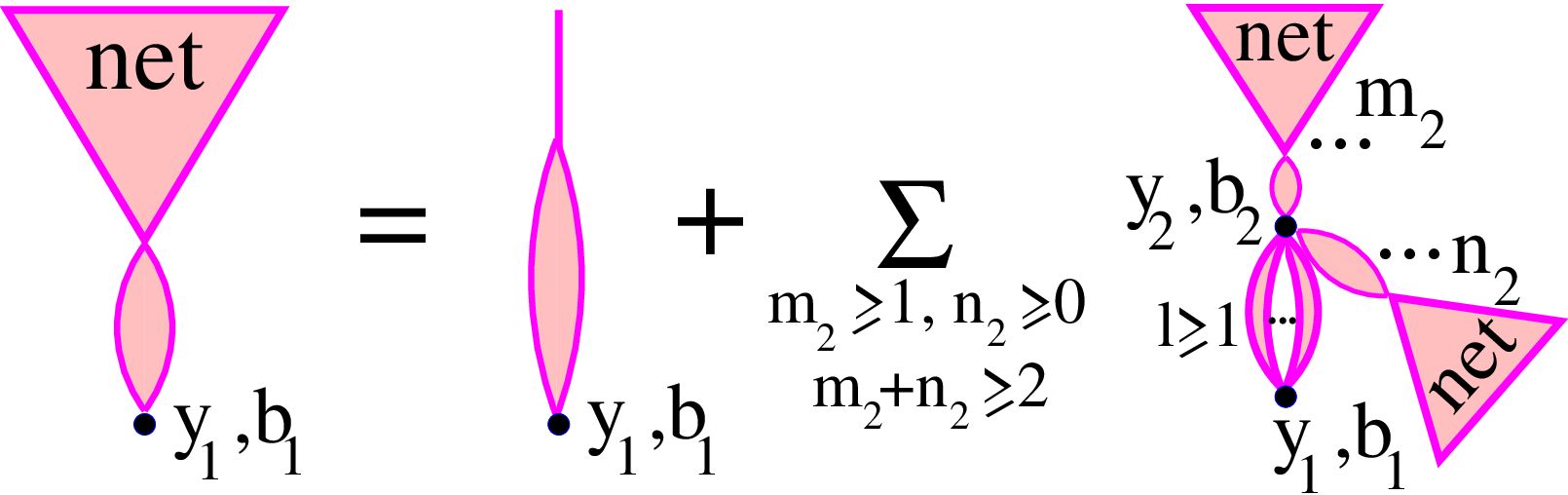
The above-defined eikonals can be used to calculate the total contribution of irreducible enhanced Pomeron graphs $\chi_{ad(jk)}^{{\rm enh}}$. As demonstrated in [12, 13], the latter can be expressed via contributions of subgraphs of certain structure, so-called “net-fans”. Those are defined by the Schwinger-Dyson equation of Fig. 3

and correspond to arbitrary irreducible ‘‘nets’’ of Pomerons, with neighboring net ‘‘cells’’ being connected to each other by 2-point sequences of Pomerons and Pomeron loops and with one vertex in the net having a fixed position in the rapidity and impact parameter space.²² 2 The 2-point sequence of Pomerons and Pomeron loops, coupled to this vertex, will be referred to as the “handle of the fan”. The corresponding equation

	$\displaystyle\chi_{a(j)|d(k)}^{{\rm net}}(y_{1},\vec{b}_{1}|Y,\vec{b})=\chi_{a(j)}^{{\rm loop}}(y_{1},b_{1})+G\int_{\xi}^{y_{1}-\xi}\!dy_{2}\int\!d^{2}b_{2}\;\left(1-e^{-\chi^{{\rm loop}}(y_{1}-y_{2},|\vec{b}_{1}-\vec{b}_{2}|)}\right)$
	$\displaystyle\times\left[\left(1-e^{-\chi_{a(j)|d(k)}^{{\rm net}}(y_{2},\vec{b}_{2}|Y,\vec{b})}\right)\;e^{-\chi_{d(k)|a(j)}^{{\rm net}}(Y-y_{2},\vec{b}-\vec{b}_{2}|Y,\vec{b})}-\chi_{a(j)|d(k)}^{{\rm net}}(y_{2},\vec{b}_{2}|Y,\vec{b})\right]$		(17)

involves the contribution $\chi^{{\rm loop}}(y_{1}-y_{2},|\vec{b}_{1}-\vec{b}_{2}|)$ of irreducible 2-point sequences of Pomerons and Pomeron loops, exchanged between the vertices $(y_{1},\vec{b}_{1})$ and $(y_{2},\vec{b}_{2})$ (2nd graph in the r.h.s. of Fig. 3), and the contribution $\chi_{a(j)}^{{\rm loop}}(y_{1},b_{1})$ of Pomeron loop sequences exchanged between the vertex $(y_{1},\vec{b}_{1})$ and hadron $a$, with a single Pomeron coupled to hadron $a$ (1st graph in the r.h.s. of the Figure). The $y_{2}$ integration in the 2nd term in the r.h.s. of (17) is performed between $\xi$ and $y_{1}-\xi$, with $\xi$ being the minimal rapidity interval for the Pomeron asymptotics to be applicable. As discussed in [20], net-fan eikonals $\chi_{a(j)|d(k)}^{{\rm net}}$ are related to parton (sea quark and gluon) distributions which are probed during hadron-hadron interaction and are thus influenced by rescattering processes on the partner hadron.

As in [14], we define the contribution $\chi^{{\rm loop}}(y_{1}-y_{2},|\vec{b}_{1}-\vec{b}_{2}|)$ and a part of it $\chi^{{\rm loop(1)}}(y_{1}-y_{2},|\vec{b}_{1}-\vec{b}_{2}|)$, corresponding to Pomeron loop sequences which start from a single Pomeron coupled to the vertex $(y_{1},\vec{b}_{1})$, via Schwinger-Dyson equations of Fig. 4,

which gives

	$\displaystyle\chi^{{\rm loop}(1)}(y_{2}-y_{1},|\vec{b}_{2}-\vec{b}_{1}|)=\chi^{\mathbb{P}}(y_{2}-y_{1},|\vec{b}_{2}-\vec{b}_{1}|)+G\int_{y_{1}+\xi}^{y_{2}-\xi}\!dy^{\prime}\int\!d^{2}b^{\prime}\;\chi^{\mathbb{P}}(y^{\prime}-y_{1},|\vec{b}^{\prime}-\vec{b}_{1}|)$
	$\displaystyle\times\left[1-e^{-\chi^{{\rm loop}}(y_{2}-y^{\prime},|\vec{b}_{2}-\vec{b}^{\prime}|)}-\chi^{{\rm loop(1)}}(y_{2}-y^{\prime},|\vec{b}_{2}-\vec{b}^{\prime}|)\right]$		(18)
	$\displaystyle\chi^{{\rm loop}}(y_{2}-y_{1},|\vec{b}_{2}-\vec{b}_{1}|)=\chi^{{\rm loop}(1)}(y_{2}-y_{1},|\vec{b}_{2}-\vec{b}_{1}|)+G\int_{y_{1+}\xi}^{y_{2}-\xi}\!dy^{\prime}\int\!d^{2}b^{\prime}\;$
	$\displaystyle\times\left[1-e^{-\chi^{{\rm loop}}(y^{\prime}-y_{1},|\vec{b}^{\prime}-\vec{b}_{1}|)}-\chi^{{\rm loop}}(y^{\prime}-y_{1},|\vec{b}^{\prime}-\vec{b}_{1}|)\right]\left[1-e^{-\chi^{{\rm loop}}(y_{2}-y^{\prime},|\vec{b_{2}}-\vec{b}^{\prime}|)}\right].$		(19)

In turn, for the contribution $\chi_{a(j)}^{{\rm loop}}(y_{1},b_{1})$ and a part of it $\chi_{a(j)}^{{\rm loop(1)}}(y_{1},b_{1})$, corresponding to irreducible Pomeron loop sequences with a single Pomeron coupled to the vertex $(y_{1},\vec{b}_{1})$, this leads to recursive equations [14]

	$\displaystyle\chi_{a(j)}^{{\rm loop}}(y_{1},b_{1})=\chi_{a(j)}^{\mathbb{P}}(y_{1},b_{1})+G\int_{\xi}^{y_{1}-\xi}\!dy^{\prime}\int\!d^{2}b^{\prime}\;\chi_{a(j)}^{\mathbb{P}}(y^{\prime},b^{\prime})$
	$\displaystyle\times\left[1-e^{-\chi^{{\rm loop}}(y_{1}-y^{\prime},|\vec{b}_{1}-\vec{b}^{\prime}|)}-\chi^{{\rm loop(1)}}(y_{1}-y^{\prime},|\vec{b}_{1}-\vec{b}^{\prime}|)\right]$		(20)
	$\displaystyle\chi_{a(j)}^{{\rm loop}(1)}(y_{1},b_{1})=\chi_{a(j)}^{\mathbb{P}}(y_{1},b_{1})+G\int_{\xi}^{y_{1}-\xi}\!dy^{\prime}\int\!d^{2}b^{\prime}\;\left[\chi_{a(j)}^{{\rm loop}}(y^{\prime},b^{\prime})-\chi_{a(j)}^{{\rm loop(1)}}(y^{\prime},b^{\prime})\right]$
	$\displaystyle\times\,\chi^{\mathbb{P}}(y_{1}-y^{\prime},|\vec{b}_{1}-\vec{b}^{\prime}|)\,.$		(21)

Finally, for the total contribution of irreducible enhanced graphs $\chi_{ad(jk)}^{{\rm enh}}$ (exchanged between eigenstates $|j\rangle$ and $|k\rangle$ of the projectile and of the target respectively) to elastic scattering amplitude one obtains [13, 14]

	$\displaystyle\chi_{ad(jk)}^{{\rm enh}}(s,b)=G\int_{\xi}^{Y-\xi}\!\!dy_{1}\!\int\!\!d^{2}b_{1}\;\left\{\left[\left(1-e^{-\chi_{a(j)|d(k)}^{{\rm net}}}\right)\left(1-e^{-\chi_{d(k)|a(j)}^{{\rm net}}}\right)-\chi_{a(j)|d(k)}^{{\rm net}}\,\chi_{d(k)|a(j)}^{{\rm net}}\right]\right.$
	$\displaystyle-\left[\chi_{a(j)|d(k)}^{{\rm net}}-\chi_{a(j)}^{{\rm loop}}(Y-y_{1},|\vec{b}-\vec{b}_{1}|)\right]\left[\left(1-e^{-\chi_{d(k)|a(j)}^{{\rm net}}}\right)e^{-\chi_{a(j)|d(k)}^{{\rm net}}}-\chi_{d(k)|a(j)}^{{\rm net}}\right]$
	$\displaystyle+\left.\chi_{d(k)}^{\mathbb{P}}(y_{1},b_{1})\left[\chi_{a(j)}^{{\rm loop}}(Y-y_{1},|\vec{b}-\vec{b}_{1}|)-\chi_{a(j)}^{{\rm loop(1)}}(Y-y_{1},|\vec{b}-\vec{b}_{1}|)\right]\right\}\!,$		(22)

where $Y=\ln(s/s_{0})$ and the omitted arguments of the eikonals read $\chi_{a(j)|d(k)}^{{\rm net}}=\chi_{a(j)|d(k)}^{{\rm net}}(Y-y_{1},\vec{b}-\vec{b}_{1}|Y,\vec{b})$, $\chi_{d(k)|a(j)}^{{\rm net}}=\chi_{d(k)|a(j)}^{{\rm net}}(y_{1},\vec{b}_{1}|Y,\vec{b})$. As demonstrated in [14], Eqs. (17-22) account for all important enhanced diagram contributions to elastic scattering amplitude.

The generalization of the treatment for nucleus-nucleus scattering amplitude is described in Appendix A.

The knowledge of the elastic scattering amplitude is far insufficient for the construction of a MC procedure for hadronic and nuclear inelastic collisions. What we need are partial cross sections for particular configurations of final states, which are defined by contributions of the corresponding unitarity cuts of elastic scattering diagrams. Those can be easily derived in the nonenhanced eikonal scheme using the Abramovskii-Gribov-Kancheli (AGK) cutting rules [22]. Considering diagrams with precisely $m\geq 1$ Pomerons being cut, each cut Pomeron corresponding to an elementary production process, and summing over any number of uncut Pomerons which describe additional elastic rescatterings, one obtains the so-called topological cross sections for hadron-hadron scattering [17, 18]:

$$\sigma_{ad}^{(m)}(s)=\int\!d^{2}b\;\sum_{j,k}C_{j/a}C_{k/d}\,\frac{\left(2\chi_{ad(jk)}^{\mathbb{P}}(s,b)\right)^{m}}{m!}\,e^{-2\chi_{ad(jk)}^{\mathbb{P}}(s,b)}.$$

(23)

The integrand in (23) can be interpreted as a probability to have precisely $m$ elementary production processes in the hadron-hadron collision at impact parameter $b$. On the other hand, combining diagrams where the cut plane passes between $n\geq 2$ Pomerons, none being cut, and choosing either elastic or inelastic states in the cut plane for the projectile and the target, one obtains either elastic $\sigma_{ad}^{{\rm el}}$ or various (low mass) diffraction cross sections. For example, for $\sigma_{ad}^{{\rm el}}$ and for single projectile hadron diffraction cross section one obtains [17]:

	$\displaystyle\sigma_{ad}^{{\rm el}}(s)=\int\!d^{2}b\;\left[\sum_{j,k}C_{j/a}C_{k/d}\,\left(1-e^{-\chi_{ad(jk)}^{\mathbb{P}}(s,b)}\right)\right]^{2}$		(24)
	$\displaystyle\sigma_{ad}^{{\rm SD(proj)}}(s)=\int\!d^{2}b\;\sum_{j,k,l,m}(C_{j/a}\,\delta_{jl}-C_{j/a}C_{l/a})\,C_{k/d}C_{m/d}\;e^{-\chi_{ad(jk)}^{\mathbb{P}}(s,b)-\chi_{ad(lm)}^{\mathbb{P}}(s,b)}.$		(25)

It is worth stressing that a configuration of the final state is defined by the structure of the unitarity cuts, here - by the number of cut Pomeron exchanges, and implies a resummation of all absorptive corrections due to virtual rescattering processes - uncut Pomeron exchanges.

Taking into account enhanced Pomeron diagrams significantly complicates the analysis and produces a variety of final state configurations, including e.g. ones with single or multiple large rapidity gaps (LRG) not covered by secondary particle production. The complete set of AGK-based cut enhanced diagrams has been derived in [13], the corresponding contributions being composed of various unitarity cuts of net-fan subgraphs, and contains cut diagrams of two types. The first class consists of cut diagrams characterized by a “tree”-like structure of cuts; such graphs are constructed coupling arbitrary numbers of cut and uncut net-fan contributions in one central (not necessarily unique) vertex, such that each cut net-fan subgraph is characterized by a “fan”-like structure of cuts [13]. The diagrams of the second kind are characterized by a “zigzag”-like structure of cuts; they are constructed in a similar way, with the important difference that at least one of the cut net-fan subgraphs has a zigzaglike structure of cuts, with subsequent Pomeron end rapidities satisfying $y_{1}>y_{2}<y_{3}>\cdots$. Treelike cut diagrams give important contributions to the total cross section and to partial cross sections of various final states; they provide main corrections to inclusive spectra of secondary particles. On the other hand, various contributions of zigzaglike cut graphs to the total cross section precisely cancel each other, moreover, as demonstrated in [14], they do not influence noticeably the rapidity gap structure of final states. Nevertheless, such diagrams provide contributions to inclusive particle spectra and to partial cross sections for particular final states. Therefore, our strategy will be to develop first a MC scheme taking into consideration treelike cut enhanced graphs only. After that, the procedure will be complemented by taking into account zigzaglike cut contributions.

As discussed above, to obtain cross sections for various final state configurations, we shall use as “building blocks” contributions of various unitarity cuts of net-fan graphs. For the moment, we are interested in the AGK-cuts of net-fans, characterized by a fanlike structure of cuts, which are defined by the Schwinger-Dyson equations of Fig. 5 ³³ 3 Here and in the following we use a slightly different graphic notation compared to Figs. 3, 4: a shaded ellipse with solid margins, positioned between the vertices $(y_{1},b_{1})$ and $(y_{2},b_{2})$, denotes a general (not necessarily irreducible) 2-point sequence of Pomerons and Pomeron loops exchanged between these vertices, with the corresponding contribution $[1-\exp(-\chi^{{\rm loop}}(y_{1}-y_{2},|\vec{b}_{1}-\vec{b}_{2}|))]$. Similarly, such an ellipse with dashed margins corresponds to the AGK cuts of such a sequence, with the contribution $2[1-\exp(-\chi^{{\rm loop}}(y_{1}-y_{2},|\vec{b}_{1}-\vec{b}_{2}|))]$. [13, 14].

The top line of the Figure defines the contribution $2\hat{\chi}_{a(j)|d(k)}^{{\rm fan}}$ of the subset of graphs in which the Pomeron loop sequence coupled to the vertex $(y_{1},b_{1})$ (the handle of the fan) is crossed by the cut plane. In turn, the equation in the bottom line gives the one of the diagrams where the handle of the fan remains uncut, $2\tilde{\chi}_{a(j)|d(k)}^{{\rm fan}}$. The total contribution of fanlike cuts of net-fans is thus $2\bar{\chi}_{a(j)|d(k)}^{{\rm fan}}=2\hat{\chi}_{a(j)|d(k)}^{{\rm fan}}+2\tilde{\chi}_{a(j)|d(k)}^{{\rm fan}}$. The first graph in the r.h.s. of the top line corresponds to all possible AGK-based cuts of the single 2-point sequence of Pomerons and Pomeron loops exchanged between the vertex $(y_{1},b_{1})$ and the projectile hadron whereas the next two diagrams in the r.h.s. of the graphic equation describe the development of the cut Pomeron net: The vertex $(y_{2},b_{2})$ couples together $\bar{m}\geq 1$ cut projectile net-fans, each one characterized by a fanlike structure of cuts, and any numbers $m,n\geq 0$ of uncut projectile and target net-fans, such that $\bar{m}+m+n\geq 2$. There one has to subtract the contributions of the next two diagrams which correspond to configurations of non-AGK type, where in all the $\bar{m}$ cut projectile net-fans connected to the vertex $(y_{2},b_{2})$ the handles of the fans remain uncut and are situated on the same side of the cut plane, together with all the $m$ uncut projectile net-fans. Finally, in the last graph in the top line of the Figure the cut plane passes between $m\geq 2$ uncut projectile net-fans, with at least one remaining on either side of the cut, such that a large rapidity gap is formed between the projectile proton and the vertex $(y_{2},b_{2})$. The diagrams in the bottom line of the Figure have a similar structure, as discussed in more detail in [13, 14].

As demonstrated in [13], the total contribution of fanlike cuts of net-fans coincides with twice the uncut one:

$\displaystyle 2\bar{\chi}_{a(j)|d(k)}^{{\rm fan}}(y_{1},\vec{b}_{1}|Y,\vec{b})=2\chi_{a(j)|d(k)}^{{\rm net}}(y_{1},\vec{b}_{1}|Y,\vec{b}),$

(26)

whereas for $2\hat{\chi}_{a(j)|d(k)}^{{\rm fan}}$ one obtains the recursive equation

	$\displaystyle 2\hat{\chi}_{a(j)|d(k)}^{{\rm fan}}(y_{1},\vec{b}_{1}|Y,\vec{b})=2\chi_{a(j)}^{{\rm loop}}(y_{1},b_{1})+2G\int_{\xi}^{y_{1}-\xi}\!dy_{2}\int\!d^{2}b_{2}\;\left(1-e^{-\chi^{{\rm loop}}(y_{1}-y_{2},|\vec{b}_{1}-\vec{b}_{2}|)}\right)$
	$\displaystyle\times\left[\left(1-e^{-\hat{\chi}_{a(j)|d(k)}^{{\rm fan}}(y_{2},\vec{b}_{2}|Y,\vec{b})}\right)e^{-2\chi_{d(k)|a(j)}^{{\rm net}}(Y-y_{2},\vec{b}-\vec{b}_{2}|Y,\vec{b})}-\hat{\chi}_{a(j)|d(k)}^{{\rm fan}}(y_{2},\vec{b}_{2}|Y,\vec{b})\right]\!.$		(27)

In Appendix B we derive also alternative representations for $2\hat{\chi}_{a(j)|d(k)}^{{\rm fan}}$, $2\tilde{\chi}_{a(j)|d(k)}^{{\rm fan}}$ which can be used in a MC procedure to generate the cut Pomeron structure of an irreducible cut diagram, to be discussed in Section 4. In addition, we obtain there subcontributions $2\bar{\chi}_{a(j)|d(k)}^{{\rm loop}}$, $2\tilde{\chi}_{a(j)|d(k)}^{{\rm loop}}$, which correspond to such cuts of net-fan graphs in which just one cut Pomeron is coupled to hadron $a$.

Using the above-defined building blocks, the complete set of cut irreducible graphs (with a treelike structure of cuts) for hadron-hadron scattering is given in Fig. 6 ⁴⁴ 4 As discussed in [13], the set of diagrams of Fig. 6 can also be represented in a form explicitly symmetric with respect to the projectile and the target. [13].

Each square bracket in the Figure corresponds to a positively defined contribution of a certain “macro-configuration” of the final state, characterized by certain topology of cut Pomerons, hence, by a definite pattern for secondary hadron production. For example, the diagrams in the first square bracket in Fig. 6 correspond to the configuration with at least two cut projectile and target net-fans ($\bar{m}\geq 2$, $\bar{n}\geq 2$) coupled together in the vertex $(y_{1},\vec{b}_{1})$, which results in a treelike structure of the final state: ⁵⁵ 5 The 2nd and 3rd graphs in the square bracket define the subtracted contributions of the cuts of non-AGK types. In each of the $\bar{m}$ cut projectile net-fans any cut Pomeron may split into a few, forming a fanlike structure (composed of cut Pomerons) developing towards the projectile hadron (in the 0s order with respect to the triple-Pomeron coupling a cut net-fan is represented by a single cut Pomeron exchanged between the hadron and the multi-Pomeron vertex); in all the $\bar{n}$ cut target net-fans such fanlike structures develop towards the target hadron. For the corresponding contribution we obtain

	$\displaystyle\bar{\Omega}_{ad(jk)}^{(1)}(s,b)=\frac{G}{2}\int_{\xi}^{Y-\xi}\!\!dy_{1}\!\int\!\!d^{2}b_{1}\;\sum_{\bar{m}=2}^{\infty}\sum_{\bar{n}=2}^{\infty}\left\{\frac{\left[2\hat{\chi}_{a(j)|d(k)}^{{\rm fan}}+2\tilde{\chi}_{a(j)|d(k)}^{{\rm fan}}\right]^{\bar{m}}}{\bar{m}!}\,e^{-2\chi_{a(j)|d(k)}^{{\rm net}}}\right.$
	$\displaystyle\times\,\frac{\left[2\hat{\chi}_{d(k)|a(j)}^{{\rm fan}}+2\tilde{\chi}_{d(k)|a(j)}^{{\rm fan}}\right]^{\bar{n}}}{\bar{n}!}\,e^{-2\chi_{d(k)|a(j)}^{{\rm net}}}-2\,\frac{\left[2\hat{\chi}_{a(j)|d(k)}^{{\rm fan}}+2\tilde{\chi}_{a(j)|d(k)}^{{\rm fan}}\right]^{\bar{m}}}{\bar{m}!}\,e^{-2\chi_{a(j)|d(k)}^{{\rm net}}}$
	$\displaystyle\times\left.\frac{\left[\tilde{\chi}_{d(k)|a(j)}^{{\rm fan}}\right]^{\bar{n}}}{\bar{n}!}\,e^{-\chi_{d(k)|a(j)}^{{\rm net}}}-2\,\frac{\left[\tilde{\chi}_{a(j)|d(k)}^{{\rm fan}}\right]^{\bar{m}}}{\bar{m}!}\,e^{-\chi_{a(j)|d(k)}^{{\rm net}}}\,\frac{\left[2\hat{\chi}_{d(k)|a(j)}^{{\rm fan}}+2\tilde{\chi}_{d(k)|a(j)}^{{\rm fan}}\right]^{\bar{n}}}{\bar{n}!}\,e^{-2\chi_{d(k)|a(j)}^{{\rm net}}}\right\}$
	$\displaystyle=\frac{G}{2}\int_{\xi}^{Y-\xi}\!\!dy_{1}\!\int\!\!d^{2}b_{1}\left\{\left[1-e^{-2\chi_{a(j)|d(k)}^{{\rm net}}}\left(1+2\chi_{a(j)|d(k)}^{{\rm net}}\right)\right]\left[1-e^{-2\chi_{d(k)|a(j)}^{{\rm net}}}\left(1+2\chi_{d(k)|a(j)}^{{\rm net}}\right)\right]\right.$
	$\displaystyle-2\left[1-e^{-2\chi_{a(j)|d(k)}^{{\rm net}}}\left(1+2\chi_{a(j)|d(k)}^{{\rm net}}\right)\right]\left[e^{\tilde{\chi}_{d(k)|a(j)}^{{\rm fan}}}-1-\tilde{\chi}_{d(k)|a(j)}^{{\rm fan}}\right]e^{-\chi_{d(k)|a(j)}^{{\rm net}}}$
	$\displaystyle-\left.2\left[e^{\tilde{\chi}_{a(j)|d(k)}^{{\rm fan}}}-1-\tilde{\chi}_{a(j)|d(k)}^{{\rm fan}}\right]e^{-\chi_{a(j)|d(k)}^{{\rm net}}}\left[1-e^{-2\chi_{d(k)|a(j)}^{{\rm net}}}\left(1+2\chi_{d(k)|a(j)}^{{\rm net}}\right)\right]\right\}\!,$		(28)

where the abbreviations are similar to the ones in (22).

The 2nd class of graphs corresponds to a LRG produced (in one particular inelastic rescattering process) between the projectile hadron and the vertex $(y_{1},\vec{b}_{1})$ and at least two cut target net-fans ($\bar{n}\geq 2$) coupled to the vertex $(y_{1},\vec{b}_{1})$, while in the third configuration the projectile and the target interchange their places. The corresponding contributions read

	$\displaystyle\bar{\Omega}_{ad(jk)}^{(2)}(s,b)=\frac{G}{2}\int_{\xi}^{Y-\xi}\!\!dy_{1}\!\int\!\!d^{2}b_{1}\left[1-e^{-\chi_{a(j)|d(k)}^{{\rm net}}}\right]^{2}$
	$\displaystyle\times\left\{\left[1-e^{-2\chi_{d(k)|a(j)}^{{\rm net}}}\left(1+2\chi_{d(k)|a(j)}^{{\rm net}}\right)\right]-2\left[e^{\tilde{\chi}_{d(k)|a(j)}^{{\rm fan}}}-1-\tilde{\chi}_{d(k)|a(j)}^{{\rm fan}}\right]e^{-\chi_{d(k)|a(j)}^{{\rm net}}}\right\}$		(29)
	$\displaystyle\bar{\Omega}_{ad(jk)}^{(3)}(s,b)=\frac{G}{2}\int_{\xi}^{Y-\xi}\!\!dy_{1}\!\int\!\!d^{2}b_{1}\left[1-e^{-\chi_{d(k)|a(j)}^{{\rm net}}}\right]^{2}$
	$\displaystyle\times\left\{\left[1-e^{-2\chi_{a(j)|d(k)}^{{\rm net}}}\left(1+2\chi_{a(j)|d(k)}^{{\rm net}}\right)\right]-2\left[e^{\tilde{\chi}_{a(j)|d(k)}^{{\rm fan}}}-1-\tilde{\chi}_{a(j)|d(k)}^{{\rm fan}}\right]e^{-\chi_{a(j)|d(k)}^{{\rm net}}}\right\}\!.$		(30)

References

• [1] P. Aurenche et al., Phys. Rev. D 45, 92 (1992).
• [2] K. Werner, F.-M. Liu and T. Pierog, Phys. Rev. C 74, 044902 (2006).
• [3] N. N. Kalmykov, S. S. Ostapchenko and A. I. Pavlov, Nucl. Phys. Proc. Suppl. 52B, 17 (1997); INP MSU 98-36/537, Moscow 1998.
• [4] E.-J. Ahn et al., Phys. Rev. D 80, 094003 (2009).
• [5] V. N. Gribov, Sov. Phys. JETP 26, 414 (1968); ibid. 29, 483 (1969).
• [6] N.N. Kalmykov, S.S. Ostapchenko, and A.I. Pavlov, Bull. Russ. Acad. Sci. Phys. 58, 1966 (1994).
• [7] H.J. Drescher et al., J. Phys. G 25, L91 (1999); S. Ostapchenko et al., ibid. 28, 2597 (2002).
• [8] L. Gribov, E. Levin, and M. Ryskin, Phys. Rep. 100, 1 (1983); A. H. Mueller and J. w. Qui, Nucl. Phys. B 268, 427 (1986).
• [9] O. V. Kancheli, JETP Lett. 18, 274 (1973); A. Schwimmer, Nucl. Phys. B 94, 445 (1975); A. Capella, J. Kaplan and J. Tran Thanh Van, ibid. 105, 333 (1976); V. A. Abramovskii, JETP Lett. 23, 228 (1976); M. S. Dubovikov and K. A. Ter-Martirosyan, Nucl. Phys. B 124, 163 (1977).
• [10] J. L. Cardi, Nucl. Phys. B 75, 413 (1974).
• [11] A. B. Kaidalov, L. A. Ponomarev and K. A. Ter-Martirosyan, Sov. J. Nucl. Phys. 44, 468 (1986).
• [12] S. Ostapchenko, Phys. Lett. B 636, 40 (2006).
• [13] S. Ostapchenko, Phys. Rev. D 77, 034009 (2008).
• [14] S. Ostapchenko, Phys. Rev. D 81, 114028 (2010).
• [15] S. Ostapchenko, in preparation.
• [16] M. L. Good and W. D. Walker, Phys. Rev. 120, 1857 (1960).
• [17] A. B. Kaidalov, Phys. Rep. 50, 157 (1979).
• [18] A. B. Kaidalov and K. A. Ter-Martirosyan, Phys. Lett. B 117, 247 (1982).
• [19] H. J. Drescher et al., Phys. Rep. 350, 93 (2001).
• [20] S. Ostapchenko, Phys. Rev. D 74, 014026 (2006).
• [21] N. N. Kalmykov and S. S. Ostapchenko, Phys. Atom. Nucl. 56, 346 (1993).
• [22] V. A. Abramovsky, V. N. Gribov and O. V. Kancheli, Sov. J. Nucl. Phys. 18, 308 (1974).
• [23] K. Werner, Phys. Rev. D 39, 780 (1989).
• [24] A. B. Kaidalov, Sov. J. Nucl. Phys. 45, 902 (1987).
• [25] K. Nakamura et al. (Particle Data Group), J. Phys. G 37, 075021 (2010).
• [26] A. Breakstone et al., Nucl. Phys. B 248, 253 (1984).
• [27] R. Battiston et al. (UA1 Collaboration), Phys. Lett. 127B, 472 (1983).
• [28] M. Bozzo et al. (UA4 Collaboration), Phys. Lett. 147B, 385 (1985); ibid. 155B, 197 (1985).
• [29] N. A. Amos et al. (E710 Collaboration), Phys. Lett. B 247, 127 (1990).
• [30] F. Abe et al. (CDF Collaboration), Phys. Rev. D 50, 5518 (1994).
• [31] M. Adamus et al., Phys. Lett. B 186, 223 (1987).
• [32] F. D. Aaron et al. (H1 and ZEUS Collaboration), JHEP 1001, 109 (2010).
• [33] S. Chekanov et al. (ZEUS Collaboration), Nucl. Phys. B 816, 1 (2009).
• [34] A. Aktas et al. (H1 Collaboration), Eur. Phys. J. C 48, 749 (2006).
• [35] N. N. Nikolaev and B. G. Zakharov, Z. Phys. C 53, 331 (1992); M. Genovese, N. N. Nikolaev and B. G. Zakharov, J. Exp. Theor. Phys. 81, 625 (1995); J. Bartels, J. R. Ellis, H. Kowalski and M. Wusthoff, Eur. Phys. J. C 7, 443 (1999).
• [36] F. Abe et al. (CDF Collaboration), Phys. Rev. D 50, 5535 (1994).
• [37] T. Affolder et al. (CDF Collaboration), Phys. Rev. Lett. 87, 141802 (2001).
• [38] A. E. Brenner et al., Phys. Rev. D 26, 1497 (1982).
• [39] J. Whitmore, Phys. Rep. 10, 273 (1974).
• [40] C. Alt et al. (NA49 Collaboration), Eur. Phys. J. C 45, 343 (2006).
• [41] G. J. Alner et al. (UA5 Collaboration), Z. Phys. C 33, 1 (1986).
• [42] C. Albajar et al. (UA1 Collaboration), Nucl. Phys. B 335, 261 (1990).
• [43] F. Abe et al. (CDF Collaboration), Phys. Rev. D 41, 2330 (1990).
• [44] F. Abe et al. (CDF Collaboration), Phys. Rev. Lett. 61 (1988) 1819.
• [45] V. Khachatryan et al. (CMS Collab.), Phys. Rev. Lett. 105 (2010) 022002.
• [46] V. A. Khoze, A. D. Martin and M. G. Ryskin, Phys. Lett. B 679, 56 (2009).
• [47] V. Berardi et al. (TOTEM Collaboration), CERN-LHCC-2004-002, Jan 2004; CERN-LHCC-2004-020, Jun 2004.
• [48] G. Aad et al. (ATLAS Collaboration), arXiv:0901.0512 [hep-ex].
• [49] U. Dersch et al. (SELEX Collaboration), Nucl. Phys. B 579, 277 (2000).
• [50] C. Alt et al. (NA49 Collaboration), Eur. Phys. J. C 49, 897 (2007).
• [51] M. Baker and K. A. Ter-Martirosian, Phys. Rep. 28, 1 (1976).
• [52] S. Ostapchenko, arXiV:hep-ph/0501093.
• [53] M. Braun, Sov. J. Nucl. Phys. 52, 164 (1990); V. A. Abramovsky and G. G. Leptoukh, ibid. 55, 903 (1992); M. Hladik et al., Phys. Rev. Lett. 86, 3506 (2001).