Mixed-Membership Stochastic Block-Models for Transactional Networks
Abstract
Transactional network data can be thought of as a list of one-to-many communications (e.g., email) between nodes in a social network. Most social network models convert this type of data into binary relations between pairs of nodes. We develop a latent mixed membership model capable of modeling richer forms of transactional network data, including relations between more than two nodes. The model can cluster nodes and predict transactions. The block-model nature of the model implies that groups can be characterized in very general ways. This flexible notion of group structure enables discovery of rich structure in transactional networks. Estimation and inference are accomplished via a variational EM algorithm. Simulations indicate that the learning algorithm can recover the correct generative model. Interesting structure is discovered in the Enron email dataset and another dataset extracted from the Reddit website. Analysis of the Reddit data is facilitated by a novel performance measure for comparing two soft clusterings. The new model is superior at discovering mixed membership in groups and in predicting transactions.
Keywords:
Email Data,keywords
and
1 Introduction
With the popularity of online social networks, discussion forums and widespread use of electronic means of communication including email and text messaging, the study of network-structured data has become quite popular.
Social network data typically consist of a group of nodes (or actors) and a list of relations between nodes. The most common models assume that relations occur between pairs of nodes, and that a relation takes a binary value (presence/absence). Such data can be conceptualized as a graph, and analogously, relations can be directed or undirected. A canonical example of such data would be a group of people (nodes) and friendship relations between them. If each person identifies their friends, then the friendship relation can be directional ( likes but does not like ).
The assumptions that relations are binary-valued and occur between pairs of nodes do not always hold for network data. In many cases, the data are transactional, with multiple instances of communication between individuals occurring over time. For example, with telephone calls, a pair of nodes is involved in a call but the relation is transactional (i.e. a list of calls), rather than being binary-valued. In email data, relations are transactional and can involve more than two nodes (one sender and one or more recipients). Depending on the type of transactional data, additional information on each transaction may be available, such as a timestamps, message content, recipient classes (e.g. To/Cc/Bcc) and other “header” information.
We focus on networks in which multiple transactions occur between nodes, and each transaction (e.g. email) has a single sender and potentially multiple recipients. Since email data is the most obvious application, we use that language to develop our model. We shall assume a fixed number () of nodes (people) in the network, and that each transaction involves at least one recipient. Additional transaction data (content, time-stamp, etc.) will not be used. Thus for a group of nodes, the observable data takes the form of a list of transactions, with each transaction having a sender and between and recipients.
Given a social network, two common tasks are discovering group structure in the network and predicting future links between nodes. Our model combines these two ideas, allowing transactions between nodes to depend on group membership (the “role” played by sender and receiver). Considering nodes in a social network, it is natural to assume that each node can potentially play different roles while interacting with different sets of nodes. It is also reasonable to assume that the likelihood of an interaction between two nodes will depend on the roles they have assumed at the time of communication. One can see that these two assumptions hold in many social networks. For example, in a network constructed from emails exchanged in an academic settings, it is easily observed that each person can choose multiple roles such as professor, teaching assistant, research assistant, student, and office staff.
We propose a hierarchical Bayesian block-model inspired by the mixed membership stochastic block-model (MMSB) [1] for transactional network data (Transactional MMSB, or TMMSB). Detailed explanation of the network structure is presented in section 2. We develop our model in section 3. We discuss inference, estimation and model choice in section 4. We review the MMSB model and other related work in section 5. We then introduce a novel performance measure for soft clustering. Simulation results and results from two datasets are presented in section 7. We conclude the paper with a summary of the model, scalability results and a discussion of future directions.
2 Data and data representations
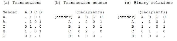
In this section, we explain structure of the network data we seek to model. A toy example of such transactional data is represented in Figure 1 (a). We have transactions, each with a sender and one or more recipient. We adopt the convention that the sender cannot be a recipient, and use a binary representation to identify recipients. Thus the first message is from A to B (represented by a in the B column and s in the C and D columns). The fourth message is from B to A and D. In general we shall assume nodes (here ) and transactions (here ).
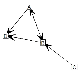
Various summaries may be derived from the raw transactions, such as a matrix of transaction counts (number of messages for each sender/receiver pair), as in Figure 1(b). This could be converted into a matrix of binary relations by thresholding the number of messages (threshold of 1 used in Figure 1(c)). This matrix of binary relations is often known as a socio-matrix. For networks with a small to moderate number of nodes, socio-matrices are visualized via a graph in which an edge indicates a directed relation between nodes. A simple visualization of the toy example is given in Figure 2.
These summaries are “lossy” representations of transactional data. For instance, from the transaction counts, we know only that B received 2 messages from A, but not that D was a co-recipient of one of these messages. The socio-matrix loses additional information, since the counts are thresholded. One thing that is not lost by these representations is the directional nature of the relations.
Representations such as the frequency matrix and socio-matrix form the basis for some network models. For instance, the latent space approach of [5] and [4] seeks a representation of nodes as points in a “latent space”, with the probability of an edge between nodes as a decreasing function of the distance between their latent positions. Extensions of the latent space model for count data [8] could be used on transaction counts. The Mixed Membership Stochastic Block-model [1] discussed in the later sections also seeks to model a binary socio-matrix.
3 Transactional Mixed Membership Block-Model
Observed network data are inherently variable, since transactions occur at random, and a finite sample of possible transactions are observed. Probabilistic generative models provide an efficient framework for modeling under uncertainty, by treating links as random and developing a probability model for their generation.
We develop a block-model for transactional network data, using the language of email data. We assume messages are sent within a network of nodes. Message has a sender , and the recipient list is represented by binary variables , where indicates node received message . For each , at least one , and if , then (i.e. a sender doesn’t send to herself).
Our model supposes the existence of groups. The probability of node sending a message to node is determined by the (unobserved) group memberships of sender and of receiver . These probabilities are collected in a interaction matrix . Element is the probability of a node in group sending a message to a node in group . This defines a basic block-model as in [11]: probability of a relation is identical between all members of two groups.
The “mixed membership” is incorporated into the model via an additional hierarchical level. Instead of assuming that each node belongs to just one group, the group membership of nodes is allowed to vary. That is, the process for generating a transaction involves random selection of group memberships for each node in the network: A group label for the “sender” and a group label for each potential “recipient”. Thus in a list of messages, node would have independent memberships sampled for it (one for each message). Conditional on these group memberships, the are independent Bernoulli outcomes. Node has a dimensional vector of membership probabilities for the classes, with . The only observables for this model are messages and senders . The matrix and group membership probabilities must all be estimated.
Our generative model for transactional data is shown in Figure 3. Each node has a mixed membership vector which is drawn from a Dirichlet prior with hyperparameter . Generating a new email involves selecting a node to be the sender from a multinomial distribution. Although the “friendship value” mechanism for selecting a sender is equivalent to a multinomial draw, we employ this more elaborate notation to enable subsequent generalization of the model. For each email , each node samples its group using its membership vector . We represent as a binary -dimensional vector with exactly one nonzero element. The recipients of this email are sampled as Bernoulli random variables. The Bernoulli probability indicates the selection of the element of corresponding to the current group membership of the sending node and the (potential) receiving node . The group membership of a node mixes over time, however for each email, each node chooses to be a member of a single group.
1. For each node , draw mixed-membership vector 2. For each node , draw its sender probability . 3. Choose : number of emails 4. For each email (a) For each node , draw (b) Pick node as sender (i.e., ) among all the nodes with probability . (c) For each node , draw
The main input parameter of the model is the number of groups . For a model with groups, other parameters that need to be estimated include the -dimensional Dirichlet parameter and a interaction matrix . Interaction matrix can be interpreted differently depending on the domain in which the model is applied. For email domain, is the probability that a node from group will receive a message from a node in group . Since the entry of the matrix corresponds to the probability of a message being sent from a member of group to a member of group , the only restriction on is that entries must be between 0 and 1. There are no restrictions on rows, columns or other collections of elements.
The arbitrary form of allows the TMMSB model to capture quite general forms of group behavior. Possibilities for include:
- 1.
Large diagonal elements, corresponding to groups that communicate among themselves, but not with other groups.
- 2.
Rows with some large entries, corresponding to groups defined by high intensity of sending communication to specific other groups.
- 3.
Columns with some large entries, corresponding to groups defined by high intensity of receiving communication from specific other groups.
- 4.
Small diagonal elements and some large off-diagonal elements, corresponding to groups that do not communicate among themselves, and are defined by similar communication patterns with members of some other groups.
Among other clustering models for socio-matrices, only the first notion of clustering is common. Section 7.1 illustrates some examples of the structures for described above.
Combining the distributions specified in this section gives a joint distribution over latent variables and the observations as
where is the set of group assignments for all nodes in all messages . is a binary matrix in which every row is a transaction and ones in each row encode the recipients of the corresponding email. Since our focus is estimating groups and membership, in the following sections we condition on senders , eliminating the need to infer the ’s.
4 Inference and Model Choice
We derive empirical Bayes estimates for the parameter and use variational approximation inference. The posterior inference in our model is intractable, nvolving a multidimensional integral and summations:
For using variational methods for inference, we pick a distribution over latent variables with free parameters. This distribution which is often called the variational distribution then approximates the true posterior in terms of Kullback-Leibler divergence by fitting its free parameters. We use a fully-factorized mean-field family of distributions as our variational distribution:
| (4.1) |
where is a Dirichlet, and is a Multinomial distribution. is the set of variational parameters that will be optimized to tighten the bound between the true posterior and variational distribution.
The updates for variational parameters and are
| (4.2) | ||||
for all transactions and all nodes , and
| (4.3) |
for all nodes . The empirical Bayes estimate for parameter is
| (4.4) |
Inference for multinomial sender probability is straightforward and thus omitted. We fix in our inference.
Algorithm 1 shows the pseudocode for the variational EM inference for the proposed model. For simplicity, a stylized version of the algorithm is presented.
The inference algorithm described above is for a fixed number of clusters . In order to choose the number of clusters, we develop a BIC criterion, composed of a log-likelihood and a penalty term.
The log-likelihood of the model is a sum of two terms, a “sending” term corresponding to selection of the sender node for each transaction and a “receiving” term for choosing group memberships and which of the other nodes receive the email. We focus on the “receiving” term. Conditional on the sender of a particular message, the likelihood for recipient nodes is equivalent to Bernoulli trials to decide whether each node receives the email (excluding the sender). Since the memberships are unobserved, we calculate a receiving probability as an average over group memberships. That is, we compute the predicted probabilities of , for each node as a sender and all the other nodes . Then, we can write the “receiving” term of the likelihood as
| (4.5) |
where is the sender node for transaction . Based on this predictive likelihood, we use the following approximation for the BIC score for choosing the number of groups:
| (4.6) |
where is the number of parameters in the model (elements of and ) and is the number of total recipients in the network.
5 Related Research
Our proposed model is inspired by the Mixed Membership Stochastic Block-model (MMSB) [1]. The MMSB model describes directional binary-valued relations between sender/receiver pairs of nodes. It seeks to model socio-matrices, such as panel (c) of Figure 1. For every sender/receiver pair, a single binary relation is observed. If , a relation has been observed; indicates no relation. The are modeled as conditionally independent Bernoulli outcomes, with . Mixed membership behaviour is incorporated by allowing node membership of nodes to change every time a directed relation is sampled. A matrix similar to represents edge probabilities between nodes in a directed binary relation.
Direct application of the MMSB model to transactional data would require simplification of the raw data. For instance, in [6], directional binary-valued relations are generated between pairs of nodes by counting the number of messages sent by and received by , and thresholding these counts at a specified level. This corresponds to the simplification from Figure 1(a) to (c). This simplification discards co-recipient information and weakens message frequency information.
Other papers have studied modeling of transactional data. Prediction of link strength in a Facebook network is studied in [7]. In their comparative study, transactional data on a network are used as features in prediction of a binary ”top friend” relation. Specific models for prediction of transactions are not developed. There has been recent work considering frequency of interactions for modeling. In [9], a stochastic block model is proposed for pairwise relation networks in which the frequency of relations are taken into account. The number of groups is inferred using Dirichlet process priors. Multiple recipient transactions are not considered in [9].
6 Novel Clustering Performance Measures
In order to assess clustering performance of our model, some new measures are needed. We consider a situation in which “ground truth” is available in the data, in the form of (possibly soft) class labels for each node. Thus measures that can assess the similarity of two different soft labels (one from a model and one from data) are needed. Although these are developed in the context of our model, these new measures can compare any two soft clusterings. These measures will be applied later in Section 7.6.
We wish to compare a predicted soft clustering (mixed membership vector in our model) with an observed mixed membership vector (e.g. normalized frequencies in the reddit case; see Section 7.4). We propose an novel extension to the evaluation measures developed in [2]. Their evaluation measure is expressed in terms of precision, recall and F-Measure values developed for overlapping clustering output. By “overlapping”, we mean a 0/1 assignment in which nodes can be assigned to multiple clusters. Our extended set of measures can be used to compare “soft” clustering results.
The proposed metrics in [2] for overlapping clustering are extensions of the BCubed metrics [3]. BCubed metrics measure precision and recall for each data point. The precision of a data point is the fraction of data points assigned to the same cluster as which belong to the same true class as . Recall for is the fraction of data points from the same true class that are assigned to the same cluster as . Extensions of precision and recall for overlapping clustering are defined as follows:
where and are two data points, is the set of classes and is the set of clusters assigned to . The expression counts the number of classes common to and . In our case, the points are not assigned to multiple clusters or do not belong to multiple classes. Each point has a membership probability vector assigned to it by the model and it has a true membership probability vector. We extend the metrics above to this case as follows:
where is the estimated membership probability vector, is the true membership probability vector for data point , and for two vectors and . Aggregate precision and recall measures are obtained by averaging over all pairs of nodes. F-measure is defined as the harmonic mean of precision and recall.
7 Examples
In this section, we present experimental results on simulated networks, an email network based on the Enron corpus and another transactional network corpus built from the social news website www.reddit.com.
7.1 Simulation Results
We simulate four transactional networks, and verify that the learned models recover the true model parameters. We are particularly interested in two parameters, membership probabilities of nodes (’s) and the interaction matrix. The simulation parameters are listed in Table 1. For , node membership probabilities are concentrated in one group. When , many nodes display mixed membership.
| Dataset | ||||
|---|---|---|---|---|
In all four cases, the recovered matrix is very close to the actual matrix used for simulation. We focus here on results for . This is the most challenging scenario, since most nodes have mixed membership. The true and recovered matrices (Table 2) are very close. In this and the other simulations large off-diagonal entries are present in , implying that some groups are defined by high volume of communication to nodes belonging to other groups.
| 0.01 | 0.2 | 0.01 | 0.01 |
| 0.01 | 0.3 | 0.2 | 0.1 |
| 0.1 | 0.01 | 0.01 | 0.3 |
| 0.1 | 0.01 | 0.01 | 0.3 |
| 0.0127 | 0.2012 | 0.0149 | 0.0115 |
| 0.0064 | 0.3055 | 0.2064 | 0.0802 |
| 0.0964 | 0.0207 | 0.0146 | 0.2959 |
| 0.0979 | 0.0243 | 0.0164 | 0.2733 |
| BIC () |
|---|
We also report the BIC scores for data simulated in the case and . In this case, we know the actual number of groups but many nodes have mixed membership. Therefore, predicting the number of groups is more challenging compared to other cases where the group memberships are close to certain. We estimate the parameters of the model using the simulated data assuming groups. Table 3 shows the BIC scores. The largest BIC values correspond to (the actual value used for simulation) and .


To assess the learned models, we use the estimated vectors to arrange the data according to the most probable grouping of nodes. The first row of Figure 4 shows the adjacency matrix for the simulated networks mentioned in Table 1. The element of the adjacency matrix is 1 if 1 or more message from node is received by node , and 0 otherwise. Nodes are ordered along rows and columns according to their most likely membership, as determined by true values of . The second row of the figure shows the same adjacency matrices, with rows and columns ordered according to estimates . Similarity between top/bottom pairs in the figure indicates that the inference algorithm is capable of recovering node memberships.
We also verify the accuracy of predictions in vectors in Figure 5, by plotting the actual elements of against the predicted values. The majority of points lie close to a 45-degree line, indicating that the “true” membership probabilities are recovered from the simulated data using the inference algorithm.


7.2 Datasets
We consider a version of the Enron email dataset provided by J. Shetty and J. Adibi 11 1 http://www.isi.edu/~adibi/Enron/Enron.htm. Their cleaned dataset consists of emails from Enron employees. We further subset the data, focusing on all messages sent in October and November, , one of the highest-volume months. This subset contains messages between distinct employees, or an average of messages sent per month by each employee. The average message has 2.45 recipients (in any of To:, CC:, BCC: fields). In the language of our paper, the sending of an email to one or more recipients is a “transaction”.
We also present results on a transactional network extracted from www.reddit.com. Reddit is a social news website where users post links to content available on the Web. These postings can generate a series of comment chains by other users. Reddit has topical sections called “subreddits”. Each subreddit focuses on a topic and there are hundreds of them, most of which are created by users. Each post is assigned to one of the available subreddits by the posting user. Each post or comment is accompanied by other information including timestamps and voting information. Because of the close community of users and their common interests, this website is a great resource for research on social networks.
We consider a transaction to be a comment or posted link and the set of its immediate follow-up comments. The user who posted the link or comment is the “sender” and all users who replied to this link or comment are “recipients”. The interpretation of is different from an email network. Here, represents the probability that a user from group is interested in links posted by a user from group .
Our dataset was derived from a crawl of the links and comments for the top popular subreddits. We subsetted this group, selecting the 10 most active subreddits and discarding all users with fewer than 250 submitted posts or comments. The resulting network has nodes and transactions. The mean number of recipients per sender is 1.15. We removed transactions from this data to use as a test set. These transactions were randomly selected from messages sent by the 10 most active nodes.
One of the features of this new dataset is the set of categories (“subreddits”). Each new post or comment is assigned to a category. Each user’s frequency of posting in the 10 subreddits characterizes that user’s activity. This 10-vector can be taken as the observed membership frequency and when normalized, as the observed membership probability vector. This information will be used as “ground truth” in section 7.6 to calculate the cluster performance measures developed in section 6.
7.3 Exploring the Enron Dataset
Our analysis of the Enron data focuses on groups. Values of BIC in Table 4 suggest this is a good group size.
Although employees have mixed membership, the membership probabilities (’s) are quite focused, with half of the employees having a maximum element of 0.85 or larger. Thus much of our analysis deals with assigning each employee to their most probable class.
| BIC () |
|---|
Grouping employees by their most probable class, we present the observed and predicted message frequency matrices in Figure 6. The groups identified by the model appear to consists of clusters of employees who email primarily to others in the same cluster. The predictions in Figure 6(b) are generated by first calculating and multiplying this by the number of messages sent by employee .


The predicted message frequency matrix in Figure 6(b) suggests that the model is capturing some characteristics of the original data. The same block diagonal cells are dark (large values) in both plots. The same horizontal band is present within group 2 for both observed and predicted matrices. This band corresponds to one employee who sent about 175 emails to the other members of group 2. This pattern, along with messages sent among members of group 2, appear to define this group. Within each group, the predicted frequencies are more homogeneous than the observed frequencies, suggesting that there remains some subject-level behavior not represented by the model.
| sending | |||||||||||||
|---|---|---|---|---|---|---|---|---|---|---|---|---|---|
| 1 | 2 | 3 | 4 | 5 | 6 | 7 | 8 | 9 | group | ||||
| 7.9 | 21.4 | 44.1 | 50 | 1.0 | 0 | 7.7 | 0 | 0 | 0 | 1.2 | 0.6 | 0 | 1 |
| 28.6 | 150.8 | 9.0 | 6 | 0 | 60.2 | 2.1 | 5.4 | 0 | 0 | 77.6 | 9.9 | 0.7 | 2 |
| 22.5 | 43.0 | 7.8 | 5 | 0 | 0 | 0.2 | 0.2 | 1.2 | 0.6 | 4.3 | 3.8 | 1.0 | 3 |
| 7.3 | 41.4 | 18.2 | 20 | 0 | 0 | 0 | 12.3 | 0 | 0 | 1.5 | 1.7 | 0.6 | 4 |
| 52.3 | 109.3 | 15.2 | 18 | 0 | 0 | 0.3 | 0 | 11.3 | 1.8 | 0 | 0 | 2.7 | 5 |
| 57.8 | 84.2 | 12.5 | 12 | 0 | 0 | 0 | 0 | 0 | 9.4 | 1.7 | 0 | 0.6 | 6 |
| 35 | 200.4 | 6.9 | 6 | 0 | 0.7 | 1.2 | 0 | 0 | 0.8 | 18.8 | 0.3 | 0.6 | 7 |
| 31.4 | 88.0 | 15.0 | 15 | 0 | 0 | 0.2 | 0 | 0.4 | 0.1 | 0.1 | 10.9 | 0 | 8 |
| 172.6 | 288.6 | 8.3 | 5 | 0 | 0 | 0 | 0 | 0.2 | 0 | 0.1 | 0 | 24.4 | 9 |
Table 5 provides several summaries of the nine groups. The first three columns are calculated using probability weights (’s) from the model. For example, if employee sends messages and has probability of belonging to group 2, then an employee in cluster 2 would send an expected messages. The activity levels vary considerably by group, as indicated by the wide range of and values. The rows of are often dominated by the diagonal element, suggesting that most identified groups tend to send to members of their own group. We comment on several interesting exceptions indicated by boxed entries in Table 5:
- •
Group 1 has lowest activity ( and in row 1), and is unlikely to receive messages from anyone except another member of group 1 (column 1 of ).
- •
Group 1 is more likely to send to group 3 than to members of its own group (row 1 entries).
- •
Group 2 is highly likely to send to members of both group 2 and 7 (row 2 entries).
- •
Group 3 has a low overall probability of sending a message, but is more likely to send to groups 7 and 8 than group 3 (row 3 entries).
We examine group 9 in more detail. Row and column 9 of (Table 5), indicate that group 9 sends messages almost exclusively to other members of group 9, and has a small but nonzero chance of receiving messages from most groups. An exception is that group 9 has negligible probability of receiving messages from groups 1 or 8. The number of messages sent and received between possible members of Group 9 is displayed in Table 6. There are 13 nodes that have probability of 0.25 or more of belonging to this group (, last column of Table 6). A block structure is quite evident in Table 6: Subgroup I (nodes 3, 4, 7, 9, 11, 18) and Subgroup II (nodes 17, 19, 27, 35, 57, 60, 61) communicate primarily amongst themselves, but very little with the other subgroup. Although it may be surprising that these two subgroups are assigned to a single group, we note that group membership is indicated by similar sending behavior, not necessarily the sending of messages to the same individuals. In this case, all nodes that have appreciable probability of belonging to group 9 share several characteristics, namely the tendency to send only to members of the same group, and the tendency to receive messages from a scattering of other groups. Inspection of suggests that no other group has this profile.
It is also interesting to note that 3 employees in Subgroup II (Dasovich-17, Steffes-19, and Shapiro-60), with large membership probabilities for group 9, were all involved in “Government relations”.
| id | 3 | 4 | 7 | 9 | 11 | 18 | 17 | 19 | 27 | 35 | 57 | 60 | 61 | oth | |
| 3 | 0 | 3 | 14 | 5 | 3 | 2 | 0 | 0 | 0 | 0 | 0 | 0 | 0 | 14 | 0.29 |
| 4 | 45 | 0 | 53 | 33 | 43 | 30 | 0 | 0 | 0 | 0 | 0 | 0 | 0 | 6 | 0.44 |
| 7 | 58 | 91 | 0 | 100 | 48 | 85 | 0 | 0 | 0 | 0 | 0 | 0 | 0 | 46 | 1.00 |
| 9 | 16 | 4 | 42 | 0 | 1 | 9 | 0 | 0 | 0 | 0 | 0 | 0 | 0 | 33 | 0.49 |
| 11 | 14 | 12 | 30 | 5 | 0 | 5 | 0 | 0 | 0 | 0 | 0 | 0 | 0 | 41 | 0.30 |
| 18 | 1 | 1 | 1 | 0 | 2 | 0 | 0 | 0 | 0 | 0 | 0 | 0 | 0 | 0 | 0.35 |
| 17 | 6 | 0 | 4 | 0 | 4 | 0 | 0 | 354 | 70 | 41 | 70 | 303 | 185 | 63 | 1.00 |
| 19 | 0 | 0 | 0 | 0 | 0 | 0 | 165 | 0 | 18 | 53 | 0 | 207 | 37 | 21 | 1.00 |
| 27 | 0 | 0 | 0 | 0 | 0 | 0 | 1 | 0 | 0 | 0 | 22 | 1 | 4 | 258 | 0.30 |
| 35 | 0 | 0 | 0 | 0 | 0 | 0 | 4 | 1 | 4 | 0 | 0 | 4 | 3 | 42 | 0.26 |
| 57 | 0 | 0 | 0 | 1 | 0 | 0 | 27 | 0 | 17 | 0 | 0 | 0 | 0 | 87 | 0.35 |
| 60 | 0 | 0 | 0 | 0 | 0 | 0 | 57 | 58 | 9 | 2 | 0 | 0 | 68 | 14 | 1.00 |
| 61 | 0 | 0 | 0 | 0 | 0 | 0 | 12 | 9 | 8 | 0 | 0 | 27 | 0 | 103 | 0.88 |
| oth | 76 | 24 | 96 | 10 | 22 | 5 | 1 | 16 | 107 | 41 | 305 | 11 | 48 |
7.4 Exploring the Reddit Dataset
| sending | ||||||||||
|---|---|---|---|---|---|---|---|---|---|---|
| 1 | 2 | 3 | 4 | 5 | 6 | group | ||||
| 10.5 | 10.8 | 80.1 | 96 | 0 | 0.9 | 1.1 | 0.1 | 0 | 1.5 | 1 |
| 17.7 | 19.3 | 51.7 | 43 | 0 | 0.6 | 3.4 | 0.1 | 0.1 | 1.2 | 2 |
| 89.5 | 119.9 | 7.9 | 5 | 0 | 0.5 | 2.5 | 0.2 | 1.7 | 0.2 | 3 |
| 22.5 | 23.9 | 37.4 | 39 | 0 | 0.3 | 6.1 | 0.2 | 1.4 | 0.1 | 4 |
| 42.3 | 48.3 | 28.5 | 29 | 0 | 0 | 5.0 | 0.1 | 2.6 | 0 | 5 |
| 28.5 | 35.3 | 42.3 | 36 | 0 | 0.5 | 0.8 | 0 | 0 | 1.9 | 6 |
As with the Enron data, we present results of an analysis with a specific . Following this analysis, we also examine predictive performance using the clustering and link prediction metrics developed in Section 6.
Table 7 shows the matrix and other summaries for a model with clusters. Summaries are the same as for the Enron data in Table 5. Entries of are considerably smaller than in the Enron case. This is due to the larger number of nodes, the smaller number of recipients per message (1.15 compared to 2.45) and the more “open” nature of discussion forums compared to email communication. The large non-diagonal entries of suggest that groups are defined in terms of between group communications as much as within. Group 1 “receives” no messages, which implies that a member of this group will make posts to a subreddit (i.e., “send” a message), but will not follow up on another post. Group 4 has low “receive” traffic as well. Group 3 is interesting in that it constitutes just a few members (5 nodes have this as their most probable class) who have very high volume of posts.
| sending | receiving group | |||||
|---|---|---|---|---|---|---|
| group | 1 | 2 | 3 | 4 | 5 | 6 |
| 1 | 0 | 0.463 | 0.088 | 0.028 | 0.013 | 0.620 |
| 2 | 0 | 0.293 | 0.267 | 0.050 | 0.018 | 0.523 |
| 3 | 0 | 0.261 | 0.195 | 0.088 | 0.478 | 0.105 |
| 4 | 0 | 0.135 | 0.482 | 0.090 | 0.412 | 0.056 |
| 5 | 0 | 0.009 | 0.393 | 0.030 | 0.752 | 0.010 |
| 6 | 0 | 0.233 | 0.061 | 0.017 | 0.007 | 0.800 |
One problem with the matrix is that it does not convey information on the expected number of recipients. For example, there is a relatively large probability (0.061) that a message sent from a member of group 4 will be received by a member of group 3. However, there are only an expected 7.9 nodes belonging to group 3, implying that the expected number of recipients would be , or about half a node. Such a calculation can be carried out for the entire matrix by multiplying column by the expected number of members in group , generating a group-size-weighted . The results are displayed in Table 8. We see that group 3 now appears less “active” since the expected number of recipients is smaller. Groups 5 and 6 have large entries on the diagonal of the group-size-weighted , suggesting they are most likely to generate posts that are responded to by members of their own group. In contrast, posts from group 4 are much more likely to generate responses from members of other groups, such as 3 and 5.
7.5 Link Prediction Results for Reddit
We compare our method with the MMSB model and a hierarchical clustering method applied to the symmetrized version of the transaction counts, e.g. Figure 1(b).
For the problem of link prediction, we use the performance measure developed in [10]. It focuses on how well a method ranks the true recipients. It uses the value of the rank at recall. A small rank indicates that the model identifies all true recipients before many non-recipients are identified. For our model ranks are generated using . For each message, we rank the nodes based on their predicted probability of being recipients of the message. We pick the rank of the last predicted recipient as performance measure for the message. The overall performance will be the average of individual performances for all messages.
Direct comparisons with link prediction are immediately possible with our model and the MMSB model, since both predict the probability of a link or transaction between two nodes. For hierarchical clustering, we must develop a similar prediction. A crude version of the matrix can be constructed using cluster labels from hierarchical clustering, and counting the number of messages sent and received by nodes with each label combination.
Fig. 7 shows the results for the three methods on the Reddit test dataset. Our method produces significantly better (i.e. lower) scores with as few as 4 groups.
7.6 Clustering Results for Reddit
As in the previous section, we compare our method with the MMSB model and a hierarchical clustering method mentioned in Section 7.5
The availability of an observed mixed membership vector (based on subreddit posting frequencies) enables us to quantify clustering accuracy in the reddit dataset. During training, the observed mixed membership vector is ignored. Using the test set described in section 7.2 and the performance measures in section 6, we can measure clustering accuracy.
In Figure 8, we compare precision, recall and F-measure for our method with values obtained for the MMSB model and a simple hierarchical clustering model. In the MMSB model, a threshold of 1 transaction was used to convert transaction counts to binary data. A hierarchical clustering method was applied to a matrix of send/receive frequencies to generate class labels for each node. The MMSB model and our model both produce mixed memberships. The hierarchical clustering method produces hard classifications. It appears that our method’s superior performance may be due to the mixed memberships and the ability to utilize co-recipient and message frequency information. Hierarchical clustering does not produce mixed membership, and the MMSB model cannot use co-recipients or message frequencies.
8 Conclusions
The key innovations of our model are the ability to probabilistically model transactional data with multiple recipients, the generalization of criteria for group membership to include communication patterns with other groups, and the development of a model in which individuals can belong to multiple groups. The variational inference algorithm is efficient for large networks, and can accurately recover network structure. The real data examples indicate that the model can extract interesting information from network data, and that it is competitive in discovering mixed memberships and in predicting transactions. We proposed a novel performance measure for comparing soft clustering results.
One issue not yet discussed is scalability of the algorithm. We studied how the TMMSB model scales with respect to the number of nodes (), transactions () and cluster size (). We fit the model to a set of simulated networks with nodes, transactions and clusters. Sufficient combinations were explored to enable estimation of a model relating time to these parameters:
This multiplicative model indicates that complexity grows much more rapidly with respect to than with respect to or . Computation times varied from 3 minutes with to 3 days with or . All computations were carried out on a Linux-based cluster with AMD Opteron CPUs (clock speeds varying from 2.6 - 3.0GHz). The fitted model, a linear regression of log time on logged , had a high , about 98.4% of variation in log time being described by a main effects model.
Our model could be extended in several ways. One shortcoming of the Bernoulli model for recipients is that it permits transactions with no recipients, an impossible outcome in email transactions. Extensions that exclude such null transactions might capture additional structure. Other transaction information such as timestamps, headers and content could be incorporated as covariates. Time-varying versions of this model could be used to discover changes in group membership and activity. This could include either varying memberships (’s) or changing numbers of groups (varying ). The simplest way to fit such a model would be to partition the time axis into intervals, and fit a separate model in each interval. More complex models could be considered. For example the MMSB model was extended to time intervals by [6], and dependence between estimated parameters was introduced via a Markov assumption, in which the parameter values were dependent between one time interval and the next.
Another extension would be to associate different group structure with the sending and receiving of messages. In the current model, the sending and receiving behavior is governed by the same groups. The additional structure would allow separation of a distribution of “message topics” from the distribution of group memberships of nodes.
An earlier version considered had additional structure, in which each transaction had a group associated with it, as well as the nodes. In this model, a group label was assigned to the transaction, and each node drew its group label. The sending node was then selected from those nodes whose current group matched the group label of the transaction. The TMMSB model described here dispenses with the additional step, simply choosing the sender from all possible nodes, and then having the message label corresponding to the group label of the sender. The additional structure would allow separation of a distribution of “message topics” from the distribution of group memberships of nodes. It does however assume that message groups and node groups have a 1:1 correspondence (same number and interpretation of categories), which might not be realistic. It is unclear whether there is sufficient information in the data to allow estimation of this additional structure, or even whether that structure serves much practical purpose.
Acknowledgements
This research was supported by the Natural Sciences and Engineering Research Council of Canada (NSERC), the Mathematics of Information Technology and Complex Systems (MITACS) and the Atlantic Computational Excellence network (ACEnet). The authors would like to thank Edo Airoldi for helpful discussions.
References
- [1] E. M. Airoldi, D. M. Blei, S. E. Fienberg, and E. P. Xing. Mixed membership stochastic blockmodels. Journal of Machine Learning Research, 9:1981–2014, 2008.
- [2] E. Amigó, J. Gonzalo, J. Artiles, and F. Artiles. A comparison of extrinsic clustering evaluation metrics based on formal constraints. Information Retrieval, 12(4):461–486, 2009.
- [3] A. Bagga and B. Baldwin. Entity-based cross-document coreferencing using the vector space model. In Proceedings of the Thirty-Sixth Annual Meeting of the Association for Computational Linguistics and Seventeenth International Conference on Computational Linguistics, pages 79–85, San Francisco, California, 1998.
- [4] M. S. Handcock, A. E. Raftery, and J. M. Tantrum. Model-based clustering for social networks. Journal Of The Royal Statistical Society Series A, 170(2):301–354, 2007.
- [5] P. Hoff, A. Raftery, and M. Handcock. Latent space approaches to social network analysis. Journal of the American Statistical Association, 97:1090–1098, 2002.
- [6] S. Huh and S. E. Fienberg. Temporally-evolving mixed membership stochastic blockmodels: Exploring the enron e-mail database. In NIPS 2008 Workshop on Analyzing Graphs: Theory and Applications.
- [7] I. Kahanda and J. Neville. Using transactional information to predict link strength in online social networks. In Proceedings of the 4th International AAAI Conference on Weblogs and Social Media.
- [8] P. N. Krivitsky and M. S. Handcock. Fitting latent cluster models for networks with latentnet. Journal of Statistical Sortware, 24(5):1–123, 2008.
- [9] K. Kurihara, Y. Kameya, and T. Sato. A frequency-based stochastic blockmodel. In Workshop on Information Based Induction Sciences, 2006.
- [10] R. Nallapati, W. Cohen, A. Ahmed, and E. Xing. Joint latent topic models for text and citations. In The 14th ACM SIGKDD International Conference on Knowledge Discovery and Data Mining, 2008.
- [11] Y. J. Wang and G. Y. Wong. Stochastic blockmodels for directed graphs. Journal of the American Statistical Association, 82(397):8–19, 1987.