We parametrize deviations of the SM electroweak sector by extending the SM Lagrangian by the most general, QED-preserving, Lorentz and $\mathcal{CP}$-invariant operators up to dimension six [41],

It is customary to express the $\kappa$-induced deviation from the SM operators^§§ § We recover the electroweak part of the SM by choosing the parameters $\kappa=1$ and $\lambda=0$. by $\Delta\kappa=\kappa-1$. The parameters $\Delta\kappa$ and $\lambda$ are related to the electric quadrupole moment $Q_{W}$ and magnetic dipole moment $\mu_{W}$ of the $W$ boson [41],

Retaining unitarity at high energies is crucial to meaningfully modeling physics beyond the SM. On the one hand, if probability conservation is violated, the cross section receives a sizable contribution from probing the matrix elements at large invariant masses, even though the parton luminosities tame the matrix elements’ unphysical growth in this particular phase space region. On the other hand, if unitarity is conserved, the phenomenology is mainly dominated by comparatively low invariant masses by the same reason. In order not to violate unitarity, the parameters $\Delta\kappa$ and $\lambda$ have to be understood as low-energy form factors, and their precise momentum dependence does depend sensitively on physics beyond the SM. However, a widely-used phenomenological parametrization is (cf. Refs. [11, 41]),

where $\Lambda$ represents the scale at which the beyond-the-SM interactions become strong, i.e. the scale at which $W$ compositeness is resolved. $p_{\gamma}$ and $p_{W}$ denote the final state momenta of the photon and the $W$, respectively. Unitarity imposes $n_{\kappa}>1/2$ and $n_{\lambda}>1$ [42]; customary choices by experimentalists are dipole profiles $n_{\kappa}=n_{\lambda}=2$ [15, 16, 10, 18, 17]. Note that we do not include anomalous ${\cal{CP}}$-violating operators since they have already been tightly constrained by measurements of the neutron electric dipole moment [43, 11].

We include the anomalous interactions by constructing purpose-built Helas routines that implement the effective Lagrangian of Eq. (8) in a straightforward way using FeynRules (Ref. [44]) to arrive at the analytical expression for the anomalous vertex function.

Throughout, we use CTEQ6M parton distributions [45] with $\alpha_{s}(m_{Z})=0.118$ at NLO, and the CTEQ6L1 set at LO. We choose $m_{Z}=91.188~\rm{GeV}$, $m_{W}=80.419~\rm{GeV}$ and $G_{F}=1.16639\times 10^{-5}~\textnormal{GeV}^{-2}$ as electroweak input parameters and derive the electromagnetic coupling $\alpha$ and the weak mixing angle from SM-tree level relations. The center-of-mass energy is fixed to $14~\rm{TeV}$ for LHC and to $1.96{\mathrm{~TeV}}$ for Tevatron collisions. We consider one family of light leptons in the final state, which we treat as massless, i.e. we quote results for $pp,p\overline{p}\rightarrow e^{-}\bar{\nu}_{e}\gamma j+X$ or $pp,p\overline{p}\rightarrow\mu^{-}\bar{\mu}_{e}\gamma j+X$ when we speak of $W^{-}\gamma+{\rm{jet}}$ production.

Jets are recombined from partons with pseudorapidity $|\eta|\leq 5$ applying the algorithm of Ref. [46] with resolution parameter $D=0.7$. The reconstructed jets are required to lie in the rapidity range

The charged lepton and the photon are required to fall into the rapidity coverage of the electromagnetic calorimeter, i.e. we impose

In order not to spoil the cancellation of the IR singularities and to minimize contributions from non-perturbative jet fragmentation associated with collinear photon-jet configurations, we apply the photon isolation criterion of Ref. [47]:

The index $i$ in Eq. (13) runs over all partons found in a cone around the photon of size $R$ in the azimuthal angle–pseudorapidity plane. The IR-safe cone size around the photon is given by $\delta_{0}$, and, in principle, $p_{T}^{\gamma}$ can be replaced by an arbitrary energy scale $\mathcal{E}$, which then determines the penetrability of the photon cone by soft QCD radiation.

In a realistic experimental setting, the photon identification efficiency depends on the number of finite-sized calorimeter towers that enter the candidate photon reconstruction (cf. Ref. [48]). It is therefore worthwhile to note that the isolation scale choice implicitly enters in the photon definition and different scale choices will be accompanied by different identification efficiencies for small values of $\delta_{0}$. A detailed investigation of this direction should include effects ranging from pile-up and underlying event to NLO-corrected jet fragmentation and is beyond the scope of this work. For values of $\delta_{0}$ much larger than the electromagnetic calorimeter cell size of $\Delta R\approx 0.04$, however, Eq. (13) is a “sliding-cut” prescription, which is experimentally well-defined on the level of already reconstructed particles. We can therefore compare the impact of the IR-safe isolation criterion to the NLO scale uncertainty, which turns out to be of order 10%. Replacing $p_{T}^{\gamma}$ in Eq. (13) by other intrinsic scales to the process, e.g. by $\max p_{T}^{j}$, corrects our NLO results at the level of $1\%$ for inclusive cuts and $\delta_{0}=0.6$ (Fig. 3). Comparing the LO and NLO inclusive distributions we find a large net increase of the differential cross section. The differences in the choice of the isolation scale, however, are only visible in the jet-photon separation distribution around the photon cone $\min R_{j\gamma}\approx\delta_{0}$. For larger separations $\min R_{j\gamma}>\delta_{0}$ we do not find any notable phenomenological impact of the isolation scale once we take into account the cross section’s residual scale dependence on $\mu_{R},\mu_{F}$. For the isolation scale ${\cal{E}}=p_{T}^{W,\gamma}=|\bm{p}_{T}^{\gamma}+\bm{p}_{T}^{\ell}+\not{\bm{p}}_{T}|$ the threshold behavior around $\delta_{0}$ changes most significantly when comparing LO and NLO distributions (we denote the neutrino’s four-momentum by $\not{p}$ in the following). The behaviour at LO is a consequence of $p^{W,\gamma}_{T}=p_{T}^{j}$ and the $W$ recoiling against the photon-jet pair if the jet is emitted around the photon cone. Therefore, probing smaller parton-photon separations effectively means increasing the transverse momentum of the $W$ for central events. The isolation scale, however, is set by the jet itself. Due to the exponential drop-off of the $p_{T}^{W}=|\bm{p}_{T}^{\ell}+\not{\bm{p}}_{T}|$ spectrum, collinear jet-photon configurations are highly attenuated for separations smaller than $\delta_{0}$ at LO, see Fig. 3. At NLO the kinematical LO correlation of the jet and $W\gamma$-system is modified by additional parton emission, which allows the $W$ to be emitted at smaller transverse momenta. Thus, QCD radiation into the photon cone around the threshold $\delta_{0}$ becomes more probable than at LO. At the same time, however, $p_{T}^{W,\gamma}$ decreases and more partons get vetoed at distances smaller than $\delta_{0}$, and a steep drop-off is still visible in $\min R_{j\gamma}$ around $\delta_{0}$ at NLO for ${\cal{E}}=p_{T}^{W,\gamma}$ in Fig. 3. In addition, we add events with a positive-definite weight to the minimum-separation distribution with the second resolved jet approximately balancing the jet-photon-$W$ system in $p_{T}$, which also modifies the $\min R_{j\gamma}$ threshold behaviour.

We now move on to investigate the general features of $W\gamma+{\rm jet}$ production with inclusive cuts on jets, photon, and lepton; we require

To avoid the collinear photon-lepton configurations we impose a finite separation in the azimuthal angle-pseudorapidity plane of

For the jet-lepton separation we choose

and for the photon isolation we impose

It is customary to also analyze the cross sections’ behavior with an additional ’no resolvable $2^{\rm{nd}}$ jet’–criterion [2], i.e. a veto on the second jet, if it gets resolved,

This allows us to identify the dominant contributions to the NLO-inclusive cross section. In addition, it was shown in Ref. [5] that this cut leads to seemingly stable exclusive $W\gamma$+jet production cross sections at the LHC. Similar observations have been made for the other diboson+jet cross sections provided in Refs. [2, 4, 3, 6, 8, 7]. The stabilization of the exclusive cross section does, however, not provide a reliable estimate of the perturbative cross sections’ uncertainties over the whole phase space. We will discuss this in more detail in Sec. 3.2.

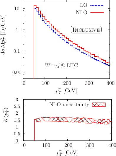
We quote the inclusive cross sections at the LHC for the chosen cuts in Tab. 1. The differences comparing $W^{+}$ to $W^{-}$ is mainly due to the different parton distributions at the LHC. The cross sections’ scale dependencies, estimated by varying $\mu_{F}=\mu_{R}$ by a factor two around $100{\mathrm{~GeV}}$, is reduced from approximately $11\%$ to $7\%$ when including the NLO QCD corrections. As already pointed out, introducing a veto on the second resolved jet, leads to considerable stabilization of the integrated NLO cross section; the one jet-exclusive cross sections (Tab. 2) exhibit scale variations of $0.5\%$ for $W^{-}\gamma$+jet and $2\%$ for $W^{+}\gamma$+jet production, respectively. Naively, this suggests that vetoing the second hard jet amounts to a perturbative stabilization of the NLO cross section at a lower exclusive rate by effectively rejecting the $\mu_{R}$-dependence of the real emission dijet contributions to the hadronic NLO $W\gamma$+jet cross sections. However, given that extra jet radiation becomes important in the tails of the transverse momentum distributions, Fig. 4, the veto introduces substantial uncertainties in this very phase space region. This can be inferred from Fig. 5, where we exemplarily examine the impact of the fixed-scale variation $\mu_{F}=\mu_{R}=50{\mathrm{~GeV}},\dots,200{\mathrm{~GeV}}$ on the photon’s transverse momentum for both inclusive and exclusive production. For completeness we note that dynamical scale choices, such as $\mu_{R}=\mu_{F}=\max p_{T}^{j}$, result in quantitatively similar uncertainty bands. While the distribution’s uncertainty band’s relative size is uniform over the entire range of the distribution for inclusive production, the jet veto stabilizes ${\mathrm{d}}\sigma_{\rm{excl}}^{\rm{NLO}}/{\mathrm{d}}p_{T}^{\gamma}$ exclusively in threshold region, which dominates the integrated exclusive rate. In fact, the distributions for $\mu=50{\mathrm{~GeV}}$ and $\mu=100{\mathrm{~GeV}}$, which are used to generate the uncertainty band in Fig. 5, intersect at $p_{T}^{\gamma}\approx 100{\mathrm{~GeV}}$ signaling an accidental cancellation of the renormalization and factorization scale dependence for the small total $K$ factors of the exclusive sample. The large uncertainty in the exclusive $p^{\gamma}_{T}$ distribution’s tail then translates into an only mild overall scale dependence $\sigma_{\rm{excl}}^{\rm{NLO}}$. Similar conclusions have been drawn for $WZ$+jet production in Ref. [8].

This is yet another example of the well-known fact that total $K$ factors and total scale variations tend to be misleading when quantifying the impact of QCD quantum corrections to a given process. A better understanding of the QCD effects can be gained from differential $K$ factors of (IR-safe) observables $\cal{O}$,

which encode the phase space dependence of the corrections, projected onto the respective observable. With unsuppressed extra jet radiation at the LHC’s large center-of-mass energy^¶¶ ¶ The proton is probed at small momentum fractions $x\sim 0.02$ at LO, which results in $\sigma^{\rm{LO}}(W^{\pm}\gamma j)/\sigma^{\rm{LO}}(W^{\pm}\gamma jj)\sim 2$ for the chosen selection criteria. Note that this is qualitatively different from the situation encountered in NLO $W\gamma$ production., the distributions’ shapes are highly altered when including NLO inclusive corrections. While the shapes of purely electroweak distributions, i.e. distributions of observables that involve only photon, lepton and missing energy, survive to NLO QCD for the most part of the phase space, semi-hadronic observables get significantly modified with respect to their LO approximations due to additional jet radiation. Representatively, we show the azimuthal angle–pseudorapidity separation of lepton and photon and the minimal distance between jet and lepton in Fig. 6. We also plot the azimuthal angle between lepton and photon and $W$ and photon in Fig. 8. The purely leptonic observables also receive sizable modifications at the edges of the phase space, which are determined by the chosen cuts. If, e.g., the $W\gamma$ system recoils against additionally emitted partons at NLO, the $W$ and the photon are forced to larger rapidity differences (Fig. 7), which communicates to the azimuthal angle–pseudorapidity separation of lepton and photon at large values. Obviously this effect cannot be buffered by the additional jet veto. It is important to note that the pseudorapidity difference of the $W$ and the photon in Fig. 7 is experimentally not observable because the neutrino’s longitudinal momentum explicitly enters the observable’s definition. We show the distribution for comparison only. All other observables do depend only on the missing transverse momentum, which is experimentally reconstructed from the event’s calorimeter entries [37].

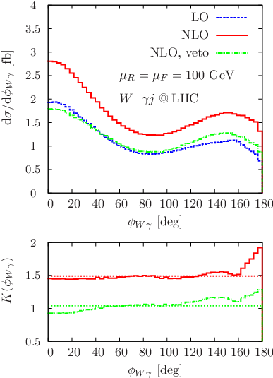
The typical signatures of $W\gamma{\rm{+jet}}$ production at the LHC are dominated by configurations close to the $p_{T}$-thresholds; the entire event is central with lepton and photon preferably emitted at small angular distances in the transverse plane. The collinear photon-lepton singularity is cut away by the requirement of Eq. (15). The photon is typically emitted collinear to the $W$ in the transverse plane. The jet recoils against the $W\gamma$ pair, and is back-to-back to the $W$ and the photon in the azimuthal angle distribution. For events with $W$ and $\gamma$ back-to-back (e.g. $|\phi_{W\gamma}|\geq 150~{\rm{deg}}$, where the inclusive NLO cross sections drops by about $80\%$ to $\sigma^{\rm{NLO}}_{\rm{incl}}=131~{\rm{fb}}$) the jets tend to balance each other at small rapidity gaps of order one. These gaps are due to the dominant $qg$- and $\bar{q}g$-induced partonic subprocesses of the dijet contribution. Due to the relatively large available phase space for additional jet emission, the corrections are particularly large for this phase space region, $K=1.6$. This is in accordance with the large differential $K$ factor around $\phi_{W\gamma}\mathrel{\raisebox{-2.58334pt}{$\stackrel{{\scriptstyle\textstyle<}}{{\sim}}$}}\pi$ in Fig. 8. Note that this is also a part of the phase space which is more sensitive to the distinct photon isolation scales. In addition, with $W$ and photon back-to-back, events with $|\phi_{W\gamma}|\geq 150~{\rm{deg}}$ can be understood as “genuine” $pp\rightarrow W\gamma+X$ events, subject to anomalous couplings’ studies^∥∥ ∥ These configurations give rise to large momentum transfers in the trilinear $WW\gamma$ coupling. The QCD corrections are therefore important to understand the deviations that result from anomalous couplings. We will discuss this in more detail in Sec. 3.4..

Anomalous couplings generically modify the $p_{T}^{\gamma}$ distribution at large values, Eq. (10). It is therefore worth commenting on the impact of the NLO corrections onto the region of phase space characterized by very large $p_{T}^{\gamma}$ already at this point. Considering energetic events in the tails of the $p_{T}$ distributions (e.g. $p_{T}^{\gamma}>1{\mathrm{~TeV}}$) the picture is quite different from the situation we have described above. Jet emission is logarithmically enhanced in the dominant gluon-induced subprocesses $qg\rightarrow W\gamma Q$ already at LO, which can easily be seen from the Altarelli-Parisi [38] approximation of collinear emission $q\rightarrow QW$ as demonstrated in Ref. [11]

for a diagonal CKM matrix. The preferred situation is therefore a collinear $W$-jet pair that recoils against the hard photon. This region of phase space receives sizable QCD corrections: The extra parton emission in these events has no preferred direction in the azimuthal angle and is kinematically unsuppressed. The $p_{T}^{W}$ distribution receives sizable corrections for the same reason. The uncertainties in this region of phase space are dominated by the dijet contribution, which is only determined to LO approximation in our calculation. Hence, our NLO correction does not improve the cross sections’ stability in this extreme region of phase space. However, as the anomalous couplings affect the $p_{T}^{\gamma}$ distribution at values much lower than $\Lambda\sim{\rm{TeV}}$, see Eq. (10), the NLO corrections give rise to perturbatively predictive deviations from the SM, see Sec. 3.4.

Vetoing the second resolved jet, Eq. (18), removes most of the characteristics of additional jet radiation. The total exclusive cross sections are tabulated in Tab. 2. Comparing the uncertainty band of the photon transverse momentum in Fig. 5 and the respective phase space dependence of the QCD corrections in Fig. 4, we conclude that perturbative stability against variations of factorization and renormalization scales of dijet-vetoed $pp\rightarrow\ell\nu\gamma j+X$ production shows up as a subtraction of a ${\cal{O}}(\alpha^{3}\alpha_{s}^{2})$ leading-order contribution (the real emission dijet contribution) from a relatively stable inclusive NLO prediction. The vetoed contribution is kinematically well-accessible and unsuppressed by QCD dynamics. The larger scale dependence of the vetoed distributions’ tails compared to inclusive production remains as an echo. At larger values of $p_{T}^{\gamma}$, exclusive production does not yield a perturbatively reliable result, which is also indicated by negative weights.

For Tevatron collisions we find a total cross section of

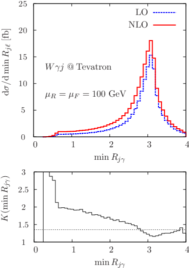
The proton and the antiproton are tested at $x\sim 0.2$ so that $q\bar{Q}$-induced subprocesses dominate the total hadronic cross section. The considerably lower center-of-mass energy compared to the LHC in combination with the cuts on the jet transverse momentum effectively introduces a jet veto, so that the Tevatron shapes resemble the NLO exclusive LHC distributions. The shapes of the transverse momentum distributions at large $p_{T}$ are overestimated by the LO approximation, yielding differential $K$ factors of order 0.5 at NLO for the distributions’ tails. Since additional jet radiation is kinematically suppressed compared to the LHC, the semi-hadronic observables typically receive smaller relative corrections around the $\sigma^{\rm{NLO}}/\sigma^{\rm{LO}}$ rescaled LO distributions. Yet, QCD-radiation effects are still sizable, and events tend to be re-distributed to smaller minimum separations of the hadronic jets with respect to the lepton and the photon, Fig. 10.

We now include anomalous couplings to the NLO $W\gamma+{\rm{jet}}$ cross section predictions. Most stringent bounds on anomalous $WW\gamma$ couplings are currently given by the combined analysis of LEP data of Ref. [17],

Both bounds are at $68\%$ confidence level, extracted from data assuming $\Lambda=2{\mathrm{~TeV}}$ and dipole profiles. Note, that both experiments are consistent with the SM prediction $\Delta\kappa_{0}=\lambda_{0}=0$. Generically, these bounds select a region in the parameter space where the QCD corrections are particularly important. This can be inferred from a scan over a wide (and experimentally ruled-out) range of anomalous parameters in Fig. 11. We choose cuts in resemblance to the selection criteria that are typically applied by the ATLAS collaboration to probe anomalous trilinear couplings, e.g., Ref. [10]

To increase the sensitivity to $\kappa_{0}$ and $\lambda_{0}$ in the experimentally allowed range, we additionally require the $W$ and the photon to be back-to-back in the transverse plane, by imposing an azimuthal angle

This cut effectively mimics “genuine” $W\gamma$ events with additional hadronic activity. Given the hard $p_{T}$ requirements, this selection criterion can be replaced by a cut on $|\phi_{\ell\gamma}|$ or $\Delta R_{\ell\gamma}$ without qualitatively changing the phenomenology (see also Figs. 7 and 8). The resulting variation of the integrated $W^{-}\gamma+{\rm{jet}}$ cross section for parameters $(\Delta\kappa_{0},\lambda_{0})$ in the range of Eq. (22) is of order 10%, Fig. 12. Comparing this variation to the uncertainty inherent to the SM expectation at the given order of perturbation theory, which, e.g., yields $\sigma\simeq 60.6~\rm{fb}$ for $\mu_{R}=\mu_{F}=50{\mathrm{~GeV}}$, we see that the cross sections’ increase due to the anomalous couplings is compatible with the SM NLO scale uncertainty, signaling a vanishing sensitivity of the total rate to $\Delta\kappa_{0},\lambda_{0}$.

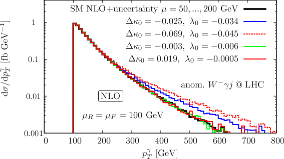
This, however, does not hold for differential distributions at large momentum transfers, e.g. for the $p_{T}^{\gamma}$ spectrum, which receives large anomalous couplings-induced modifications of the distribution’s tail. The altered spectrum is well outside the SM-uncertainty band for larger values of $(\Delta\kappa_{0},\lambda_{0})$, with a particular sensitivity to $\lambda_{0}$. Remember that $\lambda_{0}$ dials the dimension six operator in Eq. (8), which is not present in the SM. The characteristic enhancement vanishes when the anomalous parameters approach their SM values, and the shape deviations become comparable to the distribution’s uncertainty. The larger cross section at large $p_{T}^{\gamma}$ compared to the SM translates into an increased cross section for the $W\gamma$ back-to-back configurations, which is also visible in the pseudorapidity differences at small separation, Fig. 14. The anomalous couplings’ impact on this distribution is qualitatively different from the QCD corrections, which exhibit $K(p_{T}^{\gamma})<K$ for large $p_{T}^{\gamma}$. Therefore, the NLO cross section at small rapidity differences is smaller than the NLO-normalized LO distributions suggests, Fig. 7. Yet, the NLO uncertainty from integrating over the small $p_{T}$ configurations cover the anomalous couplings effect entirely, already by varying the scale within a small intervall, as indicated in Fig. 14. Given the residual anomalous couplings-induced deviations of the $p_{T}^{\gamma}$ shape, a more inclusive measurement strategy that relies on fits to the inclusive $p_{T}^{\gamma}$ spectrum or on multivariate analysis of the distributions can supplement traditional techniques and appears to be practicable. This is also motivated by the overall theoretical uncertainty of order 10% becoming comparable to the estimated experiments’ systematics at the reported order of perturbation theory.

References

- [1] J. Ohnemus, Phys. Rev. D 44 (1991) 1403, J. Ohnemus, Phys. Rev. D 44 (1991) 3477, J. Ohnemus, Phys. Rev. D 47 (1993) 940, J. Ohnemus, arXiv:hep-ph/9503389.
- [2] S. Dittmaier, S. Kallweit and P. Uwer, Phys. Rev. Lett. 100, 062003 (2008).
- [3] J. M. Campbell, R. Keith Ellis and G. Zanderighi, JHEP 0712 (2007) 056.
- [4] S. Dittmaier, S. Kallweit and P. Uwer, Nucl. Phys. B 826, 18 (2010).
- [5] F. Campanario, C. Englert, M. Spannowsky and D. Zeppenfeld, Europhys. Lett. 88, 11001 (2009).
- [6] T. Binoth, T. Gleisberg, S. Karg, N. Kauer and G. Sanguinetti, Phys. Lett. B 683 (2010) 154.
- [7] S. Ji-Juan, M. Wen-Gan, Z. Ren-You and G. Lei, Phys. Rev. D 81 (2010) 114037.
- [8] F. Campanario, C. Englert, S. Kallweit, M. Spannowsky and D. Zeppenfeld, JHEP 1007 (2010) 076.
- [9] F. Campanario, C. Englert and M. Spannowsky, Phys. Rev. D 82 (2010) 054015.
- [10] M. Dobbs, AIP Conf. Proc. 753, 181 (2005).
- [11] U. Baur, T. Han and J. Ohnemus, Phys. Rev. D 48 (1993) 5140.
- [12] L. J. Dixon, Z. Kunszt and A. Signer, Phys. Rev. D 60 (1999) 114037.
- [13] F. K. Diakonos, O. Korakianitis, C. G. Papadopoulos, C. Philippides and W. J. Stirling, Phys. Lett. B 303 (1993) 177.
- [14] E. Chapon, C. Royon and O. Kepka, Phys. Rev. D 81 (2010) 074003.
- [15] D. Levin [ATLAS Collaboration], ATL-COM-PHYS-2008-179.
- [16] T. Müller, D. Neuberg, and W. Thümmel, CERN-CMS-NOTE-2000-017 (2000).
- [17] J. Alcaraz et al. [ALEPH Collaboration and DELPHI Collaboration and L3 Collaboration and OPAL Collaboration and LEP Electroweak Working Group], arXiv:hep-ex/0612034.
- [18] V. M. Abazov et al. [D Collaboration], Phys. Rev. Lett. 100 (2008) 241805; V. M. Abazov et al. [D Collaboration], arXiv:0907.4952.
- [19] R. W. Brown, K. L. Kowalski and S. J. Brodsky, Phys. Rev. D 28 (1983) 624.
- [20] P. Fisher, U. Becker and J. Kirkby, Phys. Lett. B 356 (1995) 404; U. Baur, S. Keller and W. K. Sakumoto, Phys. Rev. D 57 (1998) 199.
- [21] K. Arnold et al., Comput. Phys. Commun. 180 (2009) 1661.
- [22] H. Murayama, I. Watanabe and K. Hagiwara, KEK-Report 91-11, 1992.
- [23] J. Alwall et al., JHEP 0709 (2007) 028.
- [24] G. P. Lepage, J. Comput. Phys. 27 (1978) 192.
- [25] T. Gleisberg, S. Hoche, F. Krauss, M. Schonherr, S. Schumann, F. Siegert and J. Winter, JHEP 0902 (2009) 007.
- [26] A. Denner, S. Dittmaier, M. Roth, and D. Wackeroth, Nucl. Phys. B 560 (1999), 33; C. Oleari and D. Zeppenfeld, Phys. Rev. D 69 (2004), 093004.
- [27] A. van Hameren, J. Vollinga and S. Weinzierl, Eur. Phys. J. C 41 (2005) 361.
- [28] A. Bredenstein, A. Denner, S. Dittmaier and S. Pozzorini, JHEP 0808 (2008) 108.
- [29] G. Passarino and M. J. G. Veltman, Nucl. Phys. B 160, 151 (1979).
- [30] A. Denner and S. Dittmaier, Nucl. Phys. B 658 (2003) 175, A. Denner and S. Dittmaier, Nucl. Phys. B 734 (2006) 62.
- [31] G. Bozzi, B. Jager, C. Oleari and D. Zeppenfeld, Phys. Rev. D 75 (2007) 073004; V. Hankele and D. Zeppenfeld, Phys. Lett. B 661 (2008) 103; F. Campanario, V. Hankele, C. Oleari, S. Prestel and D. Zeppenfeld, Phys. Rev. D 78 (2008) 094012; C. Englert, B. Jager and D. Zeppenfeld, JHEP 0903 (2009) 060; G. Bozzi, F. Campanario, V. Hankele and D. Zeppenfeld, Phys. Rev. D 81 (2010) 094030; K. Arnold, T. Figy, B. Jager and D. Zeppenfeld, JHEP 1008 (2010) 088.
- [32] T. Hahn, Comput. Phys. Commun. 140 (2001) 418.
- [33] R. Mertig, M. Bohm and A. Denner, Comput. Phys. Commun. 64 (1991) 345.
- [34] K. Hagiwara and D. Zeppenfeld, Nucl. Phys. B 313 (1989) 560.
- [35] S. Catani and M. H. Seymour, Nucl. Phys. B 485 (1997) 291 [Erratum-ibid. B 510 (1998) 503].
- [36] R. Frederix, T. Gehrmann and N. Greiner, JHEP 0809 (2008) 122.
- [37] G. Aad et al. [ATLAS Collaboration], JINST 3 (2008) S08003, G. L. Bayatian et al. [CMS Collaboration], J. Phys. G 34 (2007) 995.
- [38] V. N. Gribov and L. N. Lipatov, Sov. J. Nucl. Phys. 15 (1972) 438 [Yad. Fiz. 15 (1972) 781]; G. Altarelli and G. Parisi, Nucl. Phys. B 126 (1977) 298; Y. L. Dokshitzer, Sov. Phys. JETP 46 (1977) 641.
- [39] T. Figy, C. Oleari and D. Zeppenfeld, Phys. Rev. D 68 (2003) 073005, C. Oleari and D. Zeppenfeld, Phys. Rev. D 69 (2004) 093004.
- [40] T. Figy, V. Hankele and D. Zeppenfeld, JHEP 0802 (2008) 076.
- [41] K. Hagiwara, R. D. Peccei, D. Zeppenfeld and K. Hikasa, Nucl. Phys. B 282 (1987) 253.
- [42] U. Baur and D. Zeppenfeld, Phys. Lett. B 201 (1988) 383.
- [43] C. Amsler et al. [Particle Data Group], Phys. Lett. B 667 (2008) 1.
- [44] N. D. Christensen and C. Duhr, Comput. Phys. Commun. 180 (2009) 1614.
- [45] J. Pumplin, D. R. Stump, J. Huston, H. L. Lai, P. Nadolsky, and W. K. Tung, JHEP 0207 (2002), 012.
- [46] S. Catani, Y. L. Dokshitzer, M. H. Seymour, and B. R. Webber, Nucl. Phys. B 406 (1993), 187, S. D. Ellis and D. E. Soper, Phys. Rev. D 48 (1993) 3160.
- [47] S. Frixione, Phys. Lett. B 429 (1998) 369.
- [48] M. Escalier, F. Derue, L. Fayard, M. Kado, B. Laforge, C. Reifen, and G. Unal, CERN-ATL-PHYS-PUB-2005-018