Computing the permanental polynomials of bipartite graphs by Pfaffian orientation
Abstract
The permanental polynomial of a graph is . From the result that a bipartite graph admits an orientation such that every cycle is oddly oriented if and only if it contains no even subdivision of , Yan and Zhang showed that the permanental polynomial of such a bipartite graph can be expressed as the characteristic polynomial of the skew adjacency matrix . In this paper we first prove that this equality holds only if the bipartite graph contains no even subdivision of . Then we prove that such bipartite graphs are planar. Further we mainly show that a 2-connected bipartite graph contains no even subdivision of if and only if it is planar 1-cycle resonant. This implies that each cycle is oddly oriented in any Pfaffian orientation of a 2-connected bipartite graph containing no even subdivision of . As applications, permanental polynomials for some types of bipartite graphs are computed.
Key Words: Permanent; Permanental polynomial; Determinant; 1-cycle resonant; Pfaffian orientation.
AMS 2010 subject classification: 05C31, 05C70, 05C30, 05C75
¡¡¡¡
1 Introduction
In this article, we always consider finite and simple graphs. Let be a graph with vertex-set and edge-set . The adjacency matrix of is defined as
The permanent of an matrix is defined as
| (1) |
where denotes the set of all permutations of . The permanental polynomial of is defined as
| (2) |
where is the identity matrix of order . It is easy to see that is the sum of the principle subpermanents of [17]. It was mentioned in [2, 17] that if is a bipartite graph, then and for all ; In particular,
| (3) |
where is the number of perfect matchings of .
It was in 1981 that the permanental polynomial was firstly investigated in chemistry in [14], where some relations between the permanental polynomial and the structure of conjugated molecules were discussed. Later, Cash [3, 4] investigated the mathematical properties of the coefficients and zeros of the permanental polynomials of some chemical graphs. This suggests that the permanental polynomial encodes a variety of structural information. Gutman and Cash also demonstrated [12] several relations between the coefficients of the permanental and characteristic polynomials. See [5, 7, 13] for more about the permanental polynomials. We can compute the determinant of an matrix efficiently by Gaussian elimination. Although looks similar to , it is harder to be computed. Valiant proved [19] that it is a P-complete problem to evaluate the permanent of a -matrix. For these reasons, we want to compute the permanental polynomials of graphs by the determinant of a matrix.
Pfaffian orientations of graphs can be used to the enumeration of perfect matchings. Now we recall some definitions. A subgraph of a graph is called nice if has a perfect matching. Let be an orientation of a graph and a cycle of even length in . is oddly oriented in if contains an odd number of edges that are directed in either direction of the cycle. An orientation of is Pfaffian if every nice cycle is oddly oriented. The skew adjacency matrix of , denoted by , is defined as follows,
If a bipartite graph has a Pfaffian orientation , then [16]
| (4) |
We say an edge of a graph is oddly subdivided in a graph if is obtained from by subdividing an odd number of times. Otherwise, we say is evenly subdivided. The graph is said to be an even subdivision of a graph if can be obtained from by subdividing evenly each edge of .
Fisher and Little [8] gave a characterization of a graph that has an orientation with each cycle being oddly oriented. From this result, we have that a bipartite graph admits an orientation such that every cycle is oddly oriented if and only if it contains no even subdivision of . Accordingly, Yan and Zhang showed [21] that the permanental polynomial of such a bipartite graph can be expressed as the characteristic polynomial of the skew adjacency matrix : .
In this paper we want to investigate bipartite graphs for which the permanental polynomials can be computed by the characteristic polynomials. Following Yan and Zhang’s result, in Section 2 we obtain that a bipartite graph admits this property if and only if it has a Pfaffian orientation such that all the cycles are oddly oriented, if and only if it contains no even subdivision of .
In Section 3 we mainly characterize bipartite graphs containing no even subdivision of . The starting point of this section is to show that these graphs are planar. Then we find that if such graphs are 2-connected, they each has a bipartite ear decomposition starting with any cycle. This implies that such graphs are elementary bipartite graphs. Unexpectedly, we obtain the main result that a 2-connected bipartite graph contains no even subdivision of if and only if it is planar 1-cycle resonant. In fact, planar 1-cycle resonant graphs have already been introduced and investigated extensively in [9, 10, 11, 20]. Various characterizations [10] and constructional features [11] for planar 1-cycle resonant graphs have been given. These characterizations enable ones to design efficient algorithms to decide whether a 2-connected planar bipartite graph is 1-cycle resonant [11, 20].
From the previous main result, we have that each cycle of a 2-connected bipartite graph containing no even subdivision of is nice and is oddly oriented in any Pfaffian orientation of . Finally an algorithm [16] is recalled to give a Pfaffian orientation of a plane graph. As applications, the permanental polynomials of some types of bipartite graphs are computed. In particular, we obtain explicit expressions for permanental polynomials of two classes of graphs and .
2 A criterion for computing permanental polynomials
An elegant characterization for Pfaffian bipartite graphs was given by Little.
Theorem 2.1.
[15] A bipartite graph admits a Pfaffian orientation if and only if it does not contain an even subdivision of as a nice subgraph.
Fisher and Little gave a characterization for the existence of an orientation of a graph such that all the even cycles are oddly oriented as follows.
Theorem 2.2.
[8] A graph has an orientation under which every cycle of even length is oddly oriented if and only if the graph contains no subgraph which is, after the contraction of at most one cycle of odd length, an even subdivision of .
For bipartite graphs, we have the following immediate corollary.
Corollary 2.3.
There exists an orientation of a bipartite graph such that all the cycles of are oddly oriented if and only if contains no even subdivision of .
Based on such results, Yan and Zhang found that the permanental polynomial of a bipartite graph that has no even subdivision of can be computed by the determinant.
Theorem 2.4.
[21] Let be a bipartite graph containing no even subdivision of . Then there exists an orientation of such that
| (5) |
In fact we can show that the converse of the theorem is also valid.
Theorem 2.5.
Let be a bipartite graph of order . Then an orientation of satisfies if and only if each cycle of is oddly oriented in .
Proof.
Let
Then we have
and
where both sums range over all induced subgraphs of with vertices.
For the complete we reprove the sufficiency. If has an orientation such that every cycle is oddly oriented, then the restriction of on each induced subgraph of is a Pfaffian orientation . Hence . That means that for each . Hence .
We now prove the necessity. Suppose that has a cycle that is evenly oriented in . For convenience, let and . Now we consider the subgraph induced by the vertices of . Let be the orientation restricted on . From the definitions of permanents and determinants, we have that and , where and are the elements in the -th row and -th column of and , respectively, and both sums range over all the permutations of . For any given , if some equals zero, then . Otherwise, and or . Hence . For the cycle , we know that and since is evenly oriented. So , while . Hence .
In an analogous argument, we have that for any induced subgraph of . Hence and . ∎
Corollary 2.6.
There exists an orientation of a bipartite graph such that if and only if contains no even subdivision of .
3 Characterizations and recognition of bipartite graphs containing no even subdivision of
In this section we will characterize bipartite graphs containing no even subdivision of . We first show that such graphs are planar. Then we show that a 2-connected bipartite graph has no even subdivision of if and only if it is a planar 1-cycle resonant graph.
Theorem 3.1.
[1, Kuratowski’s theorem] A graph is planar if and only if it contains no subdivision of either or .
Lemma 3.2.
If a bipartite graph contains no even subdivision of , then it is planar.
Proof.
We prove the converse-negative proposition. Suppose that a bipartite graph is not planar. Then by Theorem 3.1 it contains a subdivision of or .
If an edge of or is oddly subdivided in , then is the path of even length in obtained by subdividing . There are two cycles , containing in or with , and the corresponding cycles in are denoted by , . Since is bipartite, in there are three pairwise internally disjoint paths of even length connecting the two endvertices of . So we obtain an even subdivision of .
If is an even subdivision of or , then or always contains as a subgraph, which corresponds to an even subdivision of in . ∎
A sequence of subgraphs of , is a bipartite ear decomposition of if is an edge , , every for is obtained from by adding an path of odd length which is openly disjoint from but its endvertices belong to . Such an ear decomposition can also be denoted as .
Lemma 3.3.
The 2-connected bipartite graph containing no even subdivision of has a bipartite ear decomposition starting with any cycle in it.
Proof.
Let be any cycle in . We want to show that has a bipartite ear decomposition starting with by induction. Let be a subgraph of obtained by successively adding ears, . If , then an edge exists in . For an edge , and lie on a common cycle since is 2-connected. Let be a path in such that the intersections of and are the both endvertices and of . If and have the same color, then is a path of even length. Since is 2-connected, has two internally disjoint paths of even length connecting and . Hence three pairwise internally disjoint paths of even length of connect and . That is, an even subdivision of exists in and a contradiction occurs. So and have different colors and is a path of odd length. Now is a subgraph of obtained by successively adding ears, . Hence has a bipartite ear decomposition starting with any cycle in it. ∎
The above result shows that such graphs relate with 1-cycle resonant graphs. A connected graph is said to be -cycle resonant if, for , any disjoint cycles in are mutually resonant, that is, there is a perfect matching of such that each of the cycles is an -alternating cycle. -cycle resonant graphs were introduced by Guo and Zhang [9] as a natural generalization of -resonant benzenoid systems, which originate from Clar’s aromatic sextet theory and Randić’s conjugated circuit model. They obtained that a -cycle resonant graph is bipartite [9]. In the following theorem, we can see that such two types of graphs are equivalent under the 2-connected condition.
Theorem 3.4.
A 2-connected bipartite graph contains no even subdivision of if and only if is planar 1-cycle resonant.
Proof.
We first prove the necessity. From Lemma 3.3, has a bipartite ear decomposition starting with any cycle in it. Because the ears s for are all of odd length, the the graph has a perfect matching which covers all the internal vertices of each . So every cycle of is nice. By Lemma 3.2 is planar. Hence is planar 1-cycle resonant.
Now we prove the sufficiency. If contains a subgraph which is an even subdivision of , then in the subgraph , there are three pairwise internally disjoint paths , and of even length joining two given vertices. Since is planar, we imbed it in the plane so that lies in the interior of the cycle . Since is 1-cycle resonant, and are nice cycles of . Hence there is an even number of vertices in the interior of and respectively. Further, since has an odd number of internal vertices, there is an odd number of vertices in the interior of . This implies that is not a nice cycle of , contradicting that is 1-cycle resonant. ∎
A connected bipartite graph is elementary if each edge is contained in a perfect matching of . For more details about such graphs see [22]. Then by Lemmas 3.2 and 3.3 or Theorem 3.4 we have the following result.
Corollary 3.5.
The 2-connected bipartite graph containing no even subdivision of is a planar and elementary bipartite graph.
A block of a connected graph is a maximal connected subgraph of without cutvertices. From Theorem 3.4 we have the following general result.
Corollary 3.6.
A connected bipartite graph contains no even subdivision of if and only if each block of is planar 1-cycle resonant.
From the proof of Theorem 3.4, we have the following result.
Corollary 3.7.
If a connected graph is a planar 1-cycle resonant graph, then it contains no even subdivision of .
We have seen in the previous theorem that 2-connected bipartite graphs containing no even subdivision of are equivalent to planar 1-cycle resonant graphs. In fact, various characterizations, the construction and recognition algorithms for planar 1-cycle resonant graphs have already been obtained in [9, 10, 11, 20]. Before stating these results, we need to give some terminology and notations.
Let be a subgraph of a connected graph . A bridge of is either an edge in with two endvertices in , or a subgraph of induced by all edges incident with a vertex in a component of . An attachment vertex of a bridge to is a vertex in which is incident with an edge in . Two bridges of a cycle avoid one another if all the attachment vertices of one bridge lie between two consecutive attachment vertices of the other bridge along .
Theorem 3.8.
Let be a 2-connected bipartite planar graph. Then the following statements are equivalent:
(1) contains no even subdivision of ,
(2) is planar 1-cycle resonant,
(3) For any cycle in , has no odd component,
(4) For any cycle in , any bridge of has exactly two attachment vertices which have different colors,
(5) For any cycle in , any two bridges of avoid one another. Moreover, for any 2-connected subgraph of with exactly two attachment vertices, the attachment vertices of have different colors.
The next result gives a structural description of planar 1-cycle resonant graphs.
Theorem 3.9.
[11] A 2-connected graph is planar 1-cycle resonant graph if and only if has a bipartite ear decomposition such that is a cycle and each () satisfies that (1) the endvertices , of have different colors in , (2) either and are adjacent in or is a vertex cut of .
This theorem can be used to construct bipartite graphs containing no even subdivision of . In addition, it derives an algorithm of time complexity , where is the number of vertices of , to determine whether a 2-connected plane graph is 1-cycle resonant; See [11] for more details.
In [20] a linear-time algorithm with respect to the number of vertices to decide whether a 2-connected plane bipartite graph is 1-cycle resonant was provided. This algorithm is designed by testing whether the attachment vertices of any bridge of the outer cycle of satisfy statement (4) in Theorem 3.8 and the attachment vertices , of any maximal 2-connected subgraph of any bridge of have different colors. If the above conditions hold, we proceed recursively for . Otherwise, is not 1-cycle resonant.
If a given planar bipartite graph is connected, we can implement the above method to each 2-connected block of to test whether it is 1-cycle resonant. If answers are all “yes”, the graph contains no even subdivision of . Hence we can present a linear time algorithm to determine whether a given planar bipartite graph contains no even subdivision of in this approach.
By the way, we turn to outerplanar graphs. A graph is outerplanar if it has an embedding into the plane with every vertex on the boundary of the exterior face. The following characterizations for outerplanar graphs were given.
Theorem 3.10.
[6] A graph is outerplanar if and only if it contains no subdivision of or .
Theorem 3.11.
[18] A graph without triangles is outerplanar if and only if it contains no subdivision of .
For bipartite graphs, we have the following characterization by Theorem 3.11.
Corollary 3.12.
A bipartite graph is outerplanar if and only if it contains no subdivision of .
From Corollary 3.12 and the characterizations of a planar 1-cycle resonant graph, we can obtain the following result immediately.
Corollary 3.13.
Let be a bipartite ear decomposition obtained by Theorem 3.9. If every ear is either a path of length 1 or joins two adjacent vertices of for , then is outerplanar. If not, contains a subdivision, but not an even subdivision, of .
4 Permanental polynomials of some graphs
In the last section some characterizations and recognition of bipartite graphs containing no even subdivision of are given. We now compute the permanental polynomials of such graphs. An algorithm is presented firstly to construct their orientations with each cycle being oddly oriented.
4.1 An orientation algorithm
The following algorithm has already been provided in [16] to construct Pfaffian orientations for plane graphs. Here we will show that, for a 2-connected bipartite graph containing no even subdivision of , each cycle of is oddly oriented in any Pfaffian orientation of it.
Algorithm 4.1.
[16]
Let be a connected plane graph.
1. Find a spanning tree in and orient it arbitrarily.
2. Let .
3. If , stop. Otherwise, take an edge of not in such that and bound
an interior face of , and orient such that an odd number of edges on the boundary of is oriented clockwise.
4. Set and . Go to step 3.
Theorem 4.2.
Theorem 4.3.
Let be a 2-connected bipartite graph containing no even subdivision of . Then each cycle is oddly oriented in a Pfaffian orientation of it.
Proof.
Since is a Pfaffian orientation of , each nice cycle is oddly oriented. From Theorem 3.4, each cycle of is nice. So each cycle of is oddly oriented in . ∎
For a connected bipartite graph containing no even subdivision of , we can give an orientation so that each cycle is oddly oriented: For each 2-connected block of , we implement Algorithm 4.1 to get its Pfaffian orientation; For each cut edge of we orient it arbitrarily. By Theorem 4.3 we can see that for such an orientation of each cycle is indeed oddly oriented.
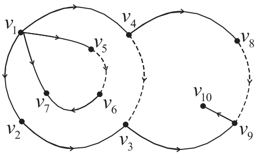
Remark 4.4.
Implementing Algorithm 4.1 directly to a connected plane bipartite graph containing no even subdivision of , we obtain a Pfaffian orientation, but cannot necessarily obtain the required orientation: an evenly oriented cycle may exist. See the graph in Figure 1 for example. The subgraph induced by the solid edges is a spanning tree with an orientation shown in Figure 1. By Algorithm 4.1, we first add the edge to and orient it from to so that the interior face bounded by it is oddly oriented. Then we add the edge and orient it from to so that the face boundary has an odd number of edges oriented clockwise along it. Finally we add the edge and orient it from to so that the face boundary has an odd number of edges oriented clockwise along it. We can see that in the resulting Pfaffian orientation, the cycles and are evenly oriented.
4.2 A computational approach
Let be a bipartite graph with . By choosing suitable ordering of vertices, the skew adjacency matrix of an oriented graph has the form
where is called the skew biadjacency matrix of . Let , , and be matrices with and . It is well-known that = Following from , we obtain that = = = . Using the result of Corollary 2.6 and Theorem 4.3, we have the following consequence.
Theorem 4.5.
Let be a 2-connected bipartite graph with containing no even subdivision of . Then , where is the skew biadjacency matrix of a Pfaffian orientation of .
4.3 Examples
We now give some examples to compute the permanental polynomials of bipartite graphs containing no even subdivision of .
Example 1. Let be the graph with pairwise internally disjoint paths of length three joining two given vertices. See Figure 2. We can see that is a bipartite graph with =. By Theorems 3.4 and 3.9 we know that contains no even subdivision of .


Lemma 4.6.
= , where .
Proof.
=
=
=. ∎
Theorem 4.7.
.
Proof.
We choose a Pfaffian orientation so that each of the paths is oriented as a directed path from vertex 1 to vertex 2 (see Figure 2). Since is 2-connected and contains no even subdivision of , by Theorem 4.5 we have that , where the skew biadjacency matrix of . As the labeling of vertices in Figure 2, the skew biadjacency matrix has the following form
Hence
=
,
by Lemma 4.6.
∎
Example 2. Let = be obtained from the Cartesian product by adding paths of length three joining the adjacent vertices and of with and ( and are the two copies of in and is the vertex of degree r in ). See Figure 3. Similar to Example 1, is a bipartite graph with = and contains no even subdivision of .


Theorem 4.8.
.
Proof.
Orientate as follows. Direct the edges in the star from the vertices of degree one to the vertex of degree and the edges in the star receive the reverse direction; Edges joining and are directed from to ; Each path of length three added to is oriented as a directed path from to (see Figure 3). It can be easily checked that each face cycle is oddly oriented. Hence is a Pfaffian orientation. Since is 2-connected and contains no even subdivision of , from Theorems 4.5 we obtain that , where the matrix is the skew biadjacency matrix of . By labeling the vertices of as shown in Figure 3, we obtain that
and
By the properties of determinants, we have that
(Since and are of order , the two matrices as above are also of order .)
(The first three matrices as above are of order and the last one is of order ; Lemma 4.6 is used repeatedly)
. ∎
Example 3. We consider outerplanar bipartite graphs. For example, see Figure 4. If all the polygons in this graph are hexagons, then the resulting graph is a catacondensed hexagonal system (see Figure 4).


Let be the graph in Figure 4 with an orientation in Figure 4 with each cycle oddly oriented. Let be the skew adjacency matrix of . We have that by Theorem 3.11 and Corollary 2.6. After computation we obtain that
Borowiechi [2] ever proved that if a bipartite graph contains no cycle of length , , and the characteristic polynomial , then . For example, we can compute . Hence the permanental polynomials of the catacondensed hexagonal system can be computed in such two methods, since they contains no cycle of length .


References
- [1] J.A. Bondy and U.S.R. Murty, Graph Theory, Springer, 2008.
- [2] M. Borowiecki, On spectrum and per-spectrum of graphs, Publ. Inst. Math., Nouv. Sér. 38(52) (1985) 31-33.
- [3] G.G. Cash, Permanental polynomials of smaller fullerenes, J. Chem. Inf. Comput. Sci. 40 (2000) 1207-1209.
- [4] G.G. Cash, The permanental polynomial, J. Chem. Inf. Comput. Sci. 40 (2000) 1203-1206.
- [5] G.G. Cash, A differential-operator approach to the permanental polynomial, J. Chem. Inf. Comput. Sci. 42 (2002) 1132-1135.
- [6] G. Chartrand and F. Harary, Planar permutation graphs, Ann. Inst. Henri Poincarè B 3 (1967) 433-438.
- [7] D.M. Cvetković, M. Doob and H. Sachs, Spectra of graphs, Academic Press, New York, 1980.
- [8] I. Fischer and C.H.C. Little, Even circuits of prescribed clockwise parity, Electron. J. Combin. 10 (2003) #R45.
- [9] X. Guo and F. Zhang, -cycle resonance graphs, Discrete Math. 135 (1994) 113-120.
- [10] X. Guo and F. Zhang, Planar -cycle resonant graphs with =1, 2, Discrete Appl. Math. 129 (2003) 383-397.
- [11] X. Guo and F. Zhang, Reducible chains of planar 1-cycle resonant graphs, Discrete Math. 275 (2004) 151-164.
- [12] I. Gutman and G.G. Cash, Relations between the permanental and characteristic polynomials of fullerenes and benzenoid hydrocarbons, MATCH Commum. Math. Comput. Chem. 45 (2002) 55-70.
- [13] Y. Huo, H. Liang and F. Bai, An efficient algorithm for computing permanental polynomials of graphs, Comput. Phys. Comm. 125 (2006) 196-203.
- [14] D. Kasum and N. Trinajstić, I. Gutman, Chemical graph theory . On the permanental polynomial, Croat. Chem. Acta 54 (1981) 321-328.
- [15] C.H.C. Little, A characterization of convertible (0,1)-matrices, J. Combin. Theory Ser. B 18 (1975) 187-208.
- [16] L. Lovász and M.D. Plummer, Matching Theory, Annals of Discrete Mathematics, Vol. 29, North-Holland, New York, 1986.
- [17] R. Merris, K.R. Rebman and W. Watkins, Permanental polynomials of graphs, Linear Algebra Appl. 38 (1981) 273-288.
- [18] M. M. Sysło, Characterization of outplanar graphs, Discrete Math. 26 (1979) 47-53.
- [19] L. Valliant, The complexity of computing the permanent, Theor. Comput. Sci. 8 (1979) 189-201.
- [20] Z. Xu and X. Guo, Construction and recognization of planar one-cycle resonant graphs, Graph Theory Notes, NY Acad. Sci. XLII (2002) 44-48.
- [21] W. Yan and F. Zhang, On the permanental polynomials of some graphs, J. Math. Chem. 35 (2004) 175-188.
- [22] H. Zhang and F. Zhang, Plane elementary bipartite graphs, Discrete Appl. Math. 105 (2000) 291-311.