Ferromagnetic Resonance in Spinor Dipolar Bose–Einstein Condensates
Abstract
We used the Gross–Pitaevskii equations to investigate ferromagnetic resonance in spin-1 Bose–Einstein condensates with a magnetic dipole-dipole interaction. By introducing the dipole interaction, we obtained equations similar to the Kittel equations used to represent ferromagnetic resonance in condensed matter physics. These equations indicated that the ferromagnetic resonance originated from dipolar interaction, and that the resonance frequency depended upon the shape of the condensate. Furthermore, spin currents driven by spin diffusions are characteristic of this system.
pacs
03.75.Mn, 03.75.NtI INTRODUCTION
Magnetic resonance (MR) as a physical concept has been applied in various fields, enabling physical, chemical, and medical experiments to obtain information on nuclear spin and electron spin systems. The concept has also provided valuable information to help understand the unknown structures of many condensed matter systems [1].
The use of MR in the study of ferromagnets, e.g. Nickel, Cobalt, and Iron, began in the 1940s. Griffiths observed that the Landé’s -factor of electrons in ferromagnets was far from the well known value, 2 [2]. In order to understand these anomalous results, Kittel theoretically introduced a demagnetizing field into the equation representing the motion of the magnetization , obtaining an equation valid in an external magnetic field , with and demagnetizing fields [3], thereby obtaining the Kittel equation,
| (1) |
Here, is the nuclear gyromagnetic ratio, and is given by the demagnetizing factors . By linearizing the magnetization from the stationary magnetization , Kittel obtained a precession of the magnetization and a precessing frequency, i.e. resonance frequency,
| (2) |
which explained the anomalous -factor. Furthermore, he found that the resonance frequency depends on the shape of a ferromagnet because depends on the shape [3]. Thus, ferromagnetic resonance (FMR) was established, and the work enabled numerous additional studies [4].
MR also plays an important role in quantum condensate systems. In superfluid 3He, the dynamics of the spin vector and the -vector are represented by the Leggett equation, which couples these vectors through magnetic dipole-dipole interactions [5]. The equation also shows not only an MR typical of condensed matter, but also a new MR that cannot be described using the equations of motion for general paramagnets and ferromagnets. This MR was used to find and phases [6]. Parallel ringing, which is an oscillation of longitudinal magnetization, was also observed [7].
Since the discovery of atomic Bose–Einstein condensates (BECs) [8, 9], BECs have been studied in optics and atomic and condensed matter physics. We have introduced MR into BECs to realize magnetic resonance imaging, a popular method of nondestructive testing. Spinor BECs are expected to be suitable for MR, since they have not only internal degrees of freedom but also magnetic properties. In particular, we are interested in magnetic dipole-dipole interactions (MDDI) in spinor BECs, which have been actively studied. The interaction between spins has a characteristic symmetry of rotation and spin, which is expected to result in a new quantum phase [10, 11, 12] and Einstein–de Haas effects [13]. Experimentally, Griesmaier et al. realized spinor dipolar condensates using 52Cr atoms, which have a larger magnetic moment than alkali atoms [14]. The shape of the condensates clearly represented the anisotropy of the interaction [15, 16]. Thus, MDDI has opened new areas of spinor condensate research.
As an introduction to MR in BECs, we numerically studied spin echo in dipolar BECs with spin-1 [19]. The spin echo is a typical phenomenon of MR, discovered by Hahn [17] and developed by Carr and Purcell [18]. Previously, we calculated the transition from Rabi oscillations to internal Josephson oscillations in spinor condensates [20]. In this paper, we consider MDDI in spin-1 BECs, examining FMR by analyzing the Gross–Pitaevskii (GP) equations.
In section II, we derive Kittel-like equations from the GP equations, and analyze them. In section III, using a single-mode approximation, we derive Kittel equations from the Kittel-like equations. The MDDI of the Kittel equations is considered as the origin of the demagnetizing field, which is phenomenologically introduced in Eq. (1). In section IV, we numerically solve the GP equations, obtaining resonance frequencies that depend upon the shape of the condensates, and spin currents driven by spin diffusion which is given by the MDDI. Finally, Sec. V is devoted to our conclusions.
II FORMULATION
In this section, we derive the equations of motion for spins from the spin-1 GP equations with an external magnetic field and an MDDI [19].
| (3) | |||||
Here, is the trapping potential, is the chemical potential, and the total density is given by . The external magnetic field is , and the components of the spin matrices are for spin-1. The interaction parameters are and for represented by s-wave scattering lengths . The dipolar coefficient is , and the unit vector is .
Under the homogeneous magnetic field , the equations can be rewritten as,
These dipolar terms are represented as,
with the integrations and given by,
| (5) |
The spin density vectors are defined as,
| (6a) | |||||
| (6b) | |||||
| (6c) | |||||
Here, is the spinor wave function.
Differentiating Eq. (6) with respect to time and utilizing Eq. (4), we can obtain the Kittel-like equation,
| (7) |
with the gyromagnetic ratio of an electron. The first term becomes,
The effective magnetic fields consist of the external magnetic field and the dipolar field , given by,
Note that Eq. (7) does not depend on spin exchange interaction, which refers to the second term with in Eq. (3). Generally, the interaction affects a spin through the effective magnetic fields of the other spins. However, exchange interaction does not appear in . Therefore, the isotropic exchange interaction does not affect MR in these condensates.
We can redefine Eq. (7) as,
| (8) |
where,
The equation of motion (8) for spins describes the properties of spin dynamics in a ferromagnetic fluid. The first, second, and third terms of Eq. (8) represent spin diffusion, spin current, and spin precession around , respectively.
Comparing Eq. (8) with Eq. (1), we noticed several differences. First, Eq. (8) was directly derived from the GP equations, whereas Eq. (1) is a phenomenological equation of magnetization. The spin density vectors in Eq. (8) are microscopically affected by other spins through the dipolar fields in the effective magnetic fields. On the other hand, the magnetization in Eq. (1) is affected by demagnetizing fields originating from macroscopically polarized magnetization in the condensed matter. Namely, Eq. (8) can describe the macroscopic demagnetizing field resulting from the microscopic dipolar field. This is a very important difference between these equations.
We initially investigated the physics of the first and second terms of Eq. (8). To simplify the discussion, we considered the equation under the condition . Thus, we derived the continuity equations,
| (9) |
where is an effective current term,
| (10a) | |||||
| (10b) | |||||
Equation (9) can also be rewritten as,
by using the volume integral and the surface integral, whose unit vector is vertical to the surface for Stokes’ theorem. The equation indicates that the expectation value of the spin matrix in the volume is conserved for the spin probability flux leaving and entering the surface.
Under , the Kittel-like equation can be reduced to the following equation,
| (11) |
where the right side of the equation breaks the conservation law of spin density. Therefore, the Kittel-like equations have two dynamics: spin precessions with frequency given by the effective magnetic field and spin currents without spin conservation. The spin currents of the system will be discussed in Sec. IV.2
III FMR under single-mode approximation
In order to study the basic properties of the second term in Eq. (7), we introduced the single-mode approximation,
| (12) |
where satisfies the eigenvalue equation with the relation . The approximation is effective when the shapes of the condensates are determined by the spin-independent terms, namely [21]. For 87Rb and 23Na, the relation is satisfied. Under this approximation, the first term of Eq. (7) vanishes, and we obtain the Kittel equation for the spatially independent spin density vector ,
| (13) |
where,
and the effective magnetic field is given by
| (14) |
Equation (13) also indicates that the spin vector precesses around . The precession frequency reveals the characteristic dynamics. Next, we consider a small deviation around the stationary solution, with , of Eq. (13), namely . Introducing this representation into Eq. (13) and linearizing the equation, we derived the following equations,
which give the resonance frequency,
| (15) |
The spin precesses with the resonance frequency , which depends on the dipolar terms .
Here, we consider the single particle density distribution , where is the aspect ratio, and discuss simple situations. For the spherical case of , the integration (14) results in , giving . The dipolar fields are canceled because of the isotropy, so that the spin precesses with Larmor frequency. For the circular plane (infinite cylinder) case of , we obtain for .
In this representation, it seems that the microscopic dipolar fields, Eq. (14), act as a macroscopic demagnetizing field to compare Eq. (2) with (15). We believe that the origin of the demagnetizing field is an MDDI. If the above discussion is correct, the dipolar coefficients should depend on the shape of the condensates. However, the single-mode approximation in spinor dipolar BECs is not effective in large-aspect-ratio condensates, as discussed by Yi and Pu [22]. Therefore, we must consider the spin dynamics beyond the approximation.
IV FMR for Numerical Calculation
IV.1 Precession dependence on the aspect ratio
In this section, we discuss FMR by numerically calculating the two-dimensional Eq. (3) under the condition of 87Rb, namely . We began calculating the spin precessions by applying a pulse to the ground state, whose spins were polarized to the uniform magnetic field trapped by with and an aspect ratio .
We investigated the dynamics of for , and with and without the MDDI. From to , a pulse was applied. Then, the spins were tilted by radians from the axis with precession. After turning off the pulse, the spins precessed around the axis, conserving . We define the notation and as indicating the expectation values of with and without an MDDI in the trap with .

First, the typical motions of spins are shown in Fig. 1. Investigating the time development of , , and , we obtained the differences between their precession frequencies, as shown in Fig. 1 (a) and (b). The differences appeared at frequencies below the Larmor frequency, given by . For , no deviation between the precessions was observed, but deviations clearly appeared as more time elapsed. In order to demonstrate that the dependence was given not by but by , we show precessions for the same aspect ratios without the MDDI in Fig. 1 (c) and (d). The precession frequency did not change without the MDDI for different values of . Therefore, the dipolar frequency depends upon the shape of the condensate.

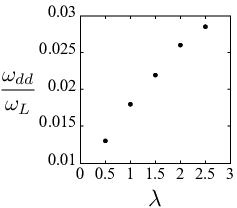
Next, we examined the effects of the MDDI on the precessions in Fig. 2. Comparing with , we observed that the MDDI caused an effective magnetic field, because the frequency of the precession with the MDDI deviated from that without the MDDI in Fig. 2 (a) to (f). Assuming that is represented approximately to with an amplitude , we extracted the dipole frequency from the waveform. Since the waveform became , the beat consisted of the large frequency and the small frequency . From Fig. 2 (h), we estimated these frequencies to obtain for respectively.
Figure 3 shows the dependence of . From the results, however, we cannot safely conclude that the dependence of the frequencies is given by changing the shape of the condensates, since the dipolar frequencies may be given by change of the density with the shape. FMR in condensed matters has been discussed in condensed matter of uniform density, even with changing shape. On the other hand, atomic BECs have tunable density and shape. Therefore, our calculations indicate characteristic of FMR in atomic cold gases.

IV.2 Spin current
We observed spin currents driven by spin diffusion, which was caused by a dependence of the dipolar field. Figure 4 shows the projections of onto the - plane for and . The precession with the MDDI lost homogeneity of the spin directions, whereas the precession without the MDDI maintained this homogeneity. This is because the precession frequency has an r dependence, specifically, .
The dipole interaction drives the spin diffusion, which is shown in Fig. 5. The figure shows as a function of at , where is the angle between the spin vector and the axis. In the dynamics with the dipole interaction for (a) and (b), the spin densities lost their angular coherence, whereas the dynamics without the dipole interactions maintained this coherence ( (c) and (d)).

The spin diffusion drives the spin current in Eq. (10), which is shown in Fig. 6. In order to explain how the spin current is driven by the spin diffusion, we considered the amplitudes of the wave functions as,
| (16b) | |||||
where the forms show the ground state of the ferromagnetic state [23]. The amplitude is represented by and the angle between the spin and the axis. We introduced this representation to demonstrate that the spin current is derived from the spin diffusion. Of course, we confirmed the validity of the ferromagnetic representation under the pulse and magnetic field by calculating directly. Therefore, it can be utilized for the polarized spin state studied in our work. The amplitudes were formed to represent , and was determined to satisfy the relation . For example, led to with , and resulted in with . The wave function can only express the ferromagnetic states, i.e. the form cannot represent the antiferromagnetic state or the polar state . This restriction of the wave function is caused by the first representation .
By introducing this representation into Eqs. (6) and (10), we can redefine as follows,
and,
| (17a) | |||||
| (17b) | |||||
where and are relative phases. Since the relation was satisfied in our calculations, we used the relation in Eqs. (17), and the spin density vector formed an azimuthal angle with the axis. Then, we derived the spin components , , and . We can therefore rewrite the spin density currents,
| (18a) | |||||
| (18b) | |||||
| (18c) | |||||
which are driven by the gradients of the angles, and , and the phase . In the precessions with MDDI, the gradients occurred because of the dipolar fields . As a result, the spin currents were clearly driven, as shown in Fig. 6. For , the spin vectors were coherent just after the applied pulse (Fig. 6 (a)). The spin densities, and , then flowed to the center of the condensates from Fig. 6 (b) to (c). Then, the densities reversed, and diffused outward from Fig. 6 (d) to (e). This oscillation was repeated. Of course, we cannot obtain the spin current without the dipolar interactions, since the gradients of and were not caused; the dynamics are shown in Fig. 7.
In order to investigate the spin fluid dynamics, we calculated the spin current for Eq. (17), as shown in Figs. 8 and 9. These figures represent from the previous calculations with and respectively. Despite the difference in the ratio, we observed two common properties in these figures. The direction of the currents changed rapidly, corresponding to the large precession frequency, and the magnitudes changed slowly with the small dipolar frequency, as shown in Fig. 10, which shows the time development of the component of . This figure indicates that the oscillation of the current direction occurred with the precession frequency, which varied in magnitude with changing dipolar frequency. Eq. (11) also indicates that the spin density was not conserved because of the effective magnetic field. Therefore, the spin currents can be driven from a source and sink in the center of the condensates, as in Figs. 8 and 9. The two common properties were insensitive to the value of . However, the change in spin density for exhibited quadratic pole motion in a scissors-like mode for mass density [24], which can be understood as an oscillation between the spin density migrating to the axis from the axis and back again, as shown in Figs. 6 (a) to (c). Therefore, the spin collective mode was caused by spin diffusions induced by the MDDI. Therefore, the spin current causes the dynamics of spin scissors-like mode, which was observed as a shrinking and expansion of the spin density in Fig. 6. The shrinking and expansion were common features for and . However, the spin currents were affected by the symmetry of the traps, as shown in Figs. 8 and 9.
From the calculations, we expected that the spin current would be observable when using the spinor BECs. Recently, spin current is focused from fields of spintronics. However, it is difficult to observe the spin current in metals and condensed matter. Atomic BECs, a macroscopic quantum phenomenon, can show the spin current clearly and directly in the dynamics of the spinor densities. Therefore, we should attempt to observe various spin currents utilizing tunable experimental parameters, i.e. interaction parameters, trap frequencies, and the number of particles.


V CONCLUSION
We investigated the properties of magnetic resonance in spinor dipolar BECs by calculating the GP equations, obtaining Kittel-like equations as the equations of motion for the spin density vector. The equations revealed two properties. One is the dynamics of the spin fluid, and the other is precession under the effective magnetic field consisting of the external magnetic fields and the dipolar fields. The magnetic resonance with the properties of the spin fluid was characteristic of this system.
In order to extract properties from the GP equations, we studied the law of conservation of spin density current without effective magnetic fields by first deriving the continuity equations from the GP equation, obtaining representations of the spin current. Second, we analytically evaluated the precession dynamics described by the Kittel equations derived from the GP equations using a single-mode approximation, where the Kittel equations show conventional FMR. The analysis clearly indicated that the origin of the FMR in the BECs is like the dipolar field, whereas the origin of the resonance in the Kittel equations for condensed matter is the demagnetizing field. Comparing the FMR of the BEC with that of the condensed matter, we concluded that the origin of the resonance was not the spin exchange interaction that causes magnetism in condensed matter, but the anisotropy of the MDDI. Finally, we numerically calculated the GP equations, representing the dynamics with the two common properties. The characteristic dynamics showed that the effective magnetic field introduced spin diffusion into the Larmor precession, driving the spin-current-like scissors modes.
The relation between the spin current and FMR has not yet been discussed for typical FMR. Therefore, it is important to study spin current in condensates. We also believe that the study of spin current will be useful for the development of spintronics, because it is difficult to directly observe spin currents in condensed matter spintronics.
VI ACKNOWLEDGMENT
M. Y. acknowledges the support of a Research Fellowship of the Japan Society for the Promotion of Science for Young Scientists (Grant No. 209928). M. T. acknowledges the support of a Grant-in Aid for Scientific Research from JSPS (Grant No. 21340104).
References
- [1] C. P. Slichter, Principles of Magnetic Resonance, (Berlin: Springer–Verlag, 1990).
- [2] J. H. E. Griffiths, Nature 158, 670 (1946).
- [3] C. Kittel, Phys. Rev. 71, 270 (1947) ; ibid. 73, 155 (1948).
- [4] C. Kittel, Introduction to Solid State Physics, 8th ed. (John Wiley and Sons Inc., USA, 2005)
- [5] A. J. Leggett, Rev. Mod. Phys. 47, 331 (1975).
- [6] D. Vollhard and P. Wlfle, The Superflluid Phasess of Helium 3 (Taylor and Francis, London, 1990).
- [7] R. A. Webb, R. L. Kleinberg, and J. C. Wheatley, Phys. Rev. Lett. 33, 145 (1974).
- [8] K. B. Davis, M. -O. Mewes, M. R. Andrews, N. J. van Druten, D. S. Durfee, D. M. Kurn and W. Ketterle, Phys. Rev. Lett. 75, 3969 (1995).
- [9] M. H. Anderson, J. R. Ensher, M. R. Matthews, C. E. Wieman and E. A. Cornell, Science 269, 198 (1995).
- [10] S. Yi, L. You and H. Pu, Phys. Rev. Lett. 93, 040403 (2004)
- [11] Y. Kawaguchi, H. Saito and M. Ueda, Phys. Rev. Lett. 97, 130404(2006).
- [12] H. Mäkelä and K. -A. Suominen, Phys. Rev. A 75, 033610 (2007).
- [13] Y. Kawaguchi, H. Saito and M. Ueda, Phys. Rev. Lett. 96, 080405 (2006).
- [14] A. Griesmaier, J. Werner, S. Hensler, J. Stuhler, and T. Pfau, Phys. Rev. Lett. 94, 160401 (2005).
- [15] J. Stuhler, A. Griesmaier, T. Koch, M. Fattori, T. Pfau, S. Giovanazzi, P. Pedri, and L. Santos, Phys. Rev. Lett. 95, 150406 (2005).
- [16] T. Lahaye, T. Koch, B. Fröhlich, M. Fattori, J. Metz, A. Griesmaier, S. Giovanazzi, and T. Pfau, Nature 448, 672 (2007).
- [17] E. L. Hahn, Phys. Rev. 80, 580 (1950).
- [18] H. Y. Carr and E. M. Purcell, Phys. Rev. 94, 630 (1954).
- [19] M. Yasunaga and M. Tsubota, Phys. Rev. Lett. 101 220401 (2008).
- [20] M. Yasunaga and M. Tsubota, J. Low Tem. Phys. 158, 51 (2010).
- [21] W. Zhang, D. L. Zhou, M. -S. Chang, M. S. Chapman, and L. You, Phys. Rev. A 72, 013602 (2005).
- [22] S. Yi and H. Pu, Phys. Rev. Lett. 97, 020401 (2006).
- [23] T. -L. Ho, Phys. Rev. Lett. 81, 742 (1998).
- [24] C. J. Pethick and H. Smith, Bose-EInstein Condensation in Dilute Gases, 2nd ed. (Cambridge, New York, 2008).