arXiv:1010.1074
ABSTRACT
Recently, Cai and Su [Phys. Rev. D 81, 103514 (2010)] found that the sign of interaction in the dark sector changed in the approximate redshift range of , by using a model-independent method to deal with the observational data. In fact, this result raises a remarkable problem, since most of the familiar interactions cannot change their signs in the whole cosmic history. Motivated by the work of Cai and Su, we have proposed a new type of interaction in a previous work [H. Wei, Nucl. Phys. B 845, 381 (2011)]. The key ingredient is the deceleration parameter in the interaction , and hence the interaction can change its sign when our universe changes from deceleration () to acceleration (). In the present work, we consider the cosmological constraints on this new type of sign-changeable interactions, by using the latest observational data. We find that the cosmological constraints on the model parameters are fairly tight. In particular, the key parameter can be constrained to a narrow range.
Cosmological Constraints on the Sign-Changeable Interactions
pacs
98.80.Es, 95.36.+x, 98.80.-kI Introduction
In the dark energy cosmology [1], the well-known cosmological coincidence problem has an important position. This problem asks: why are we living in an epoch in which the densities of dark energy and matter are comparable? Since their densities scale differently with the expansion of our universe, there should be some fine-tunings. To alleviate this coincidence problem, it is natural to consider the possible interaction between dark energy and dark matter in the literature (see e.g. [2, 3, 4, 5, 6, 7, 8, 9, 10, 11, 12]). In fact, since the natures of both dark energy and dark matter are still unknown, there is no physical argument to exclude the possible interaction between them. On the contrary, some observational evidences of the dark sector interaction have been found recently [13, 14]. In the literature, it is usual to assume that dark energy and dark matter interact through a coupling term , according to
| (1) | |||
| (2) |
where and are the densities of dark matter and dark energy (we assume that the baryon component can be ignored); is the pressure of dark energy; is the Hubble parameter; is the scale factor (we have set ; the subscript “0” indicates the present value of corresponding quantity; is the redshift); a dot denotes the derivative with respect to cosmic time . Note that Eqs. (1) and (2) preserve the total energy conservation equation , where . Since there is no natural guidance from fundamental physics on the interaction , one can only discuss it to a phenomenological level. This is the realistic status of the interacting dark energy models so far.
The most familiar interactions extensively considered in the literature (see e.g. [2, 3, 4, 5, 6, 7, 8, 9, 10, 11, 12]) include , , and . It is easy to see that these interactions are always positive or negative and hence cannot give the possibility to change their signs in the whole cosmic history. However, recently Cai and Su [15] found that the sign of interaction changed in the approximate redshift range of , by using a model-independent method to deal with the observational data. Obviously, this result raises a remarkable problem. Motivated by the work of Cai and Su, we have proposed a new type of interaction in a previous work [16], which is given by
| (3) |
where and are both dimensionless constants; the energy density could be , and for examples; the deceleration parameter
| (4) |
Obviously, this new type of interaction can change its sign when our universe changes from deceleration () to acceleration (). In fact, the deceleration parameter in is the key ingredient of this new interaction, which makes our proposal different from the previous ones considered in the literature. Note that the term in is introduced from the dimensional point of view (we refer to [16] for details). One can remove this term by setting , and then becomes simply (in fact this is the very case which will be considered in the followings).
Since the appearance of the deceleration parameter in the interaction looks speculative to some extent, we would like to say some words before going further. Firstly, as is well known, in the literature there is no natural guidance from fundamental physics on the interaction , one can only discuss it to a phenomenological level. In this sense, the other familiar interactions extensively considered in the literature have no better origin from the fundamental physics than the one proposed in Eq. (3). Secondly, we note that from Eq. (4) and from the Friedmann equation. Thus, one can regard the deceleration parameter as a function of the total energy density and its derivative. In this sense, the interaction is not so unusual, since it is reasonable to image that depends on the energy densities of dark energy and matter. Finally, while the familiar interactions extensively considered in the literature (such as , , and ) cannot give the possibility to change their signs in the whole cosmic history, our proposal in Eq. (3) provides a possible way out. So, we consider that it deserves further investigation.
In [16], we have studied the cosmological evolution of quintessence and phantom with this new type of sign-changeable interactions, and found some interesting results. In the present work, we would like to consider the cosmological constraints on this new type of sign-changeable interactions, by using the latest observational data. For simplicity, in this work, we restrict ourselves to the decaying model (see e.g. [17] and references therein), namely, the role of dark energy is played by the decaying vacuum energy. In this case, Eq. (2) becomes
| (5) |
The Friedmann and Raychaudhuri equations are given by
| (6) | |||
| (7) |
where . Notice that we consider a flat Friedmann-Robertson-Walker (FRW) universe throughout this work. In Sec. II, we briefly introduce the latest observational data which will be used in this work. In Sec. III, we consider the cosmological constraints on three particular sign-changeable interactions, i.e.,
| (8) | |||
| (9) | |||
| (10) |
Finally, some brief concluding remarks are given in Sec. IV.
II Observational data
In the present work, we will consider the latest cosmological observations, namely, the 557 Union2 Type Ia Supernovae (SNIa) dataset [18], the shift parameter from the Wilkinson Microwave Anisotropy Probe 7-year (WMAP7) data [19], and the distance parameter of the measurement of the baryon acoustic oscillation (BAO) peak in the distribution of SDSS luminous red galaxies [20, 21].
The data points of the 557 Union2 SNIa compiled in [18] are given in terms of the distance modulus . On the other hand, the theoretical distance modulus is defined as
| (11) |
where and is the Hubble constant in units of , whereas
| (12) |
in which , and denotes the model parameters. Correspondingly, the from the 557 Union2 SNIa is given by
| (13) |
where is the corresponding error. The parameter is a nuisance parameter but it is independent of the data points. One can perform an uniform marginalization over . However, there is an alternative way. Following [22, 23], the minimization with respect to can be made by expanding the of Eq. (13) with respect to as
| (14) |
where
Eq. (14) has a minimum for at
| (15) |
Since obviously, we can instead minimize which is independent of .
There are some other relevant observational data, such as the observations of cosmic microwave background (CMB) anisotropy [19] and large-scale structure (LSS) [20]. However, using the full data of CMB and LSS to perform a global fitting consumes a large amount of computation time and power. As an alternative, one can instead use the shift parameter from the CMB, and the distance parameter of the measurement of the BAO peak in the distribution of SDSS luminous red galaxies. In the literature, the shift parameter and the distance parameter have been used extensively. It is argued that they are model-independent [24], while and contain the main information of the observations of CMB and BAO, respectively.
As is well known, the shift parameter of the CMB is defined by [24, 25]
| (16) |
where is the present fractional energy density of pressureless matter; the redshift of recombination which has been updated in the Wilkinson Microwave Anisotropy Probe 7-year (WMAP7) data [19]. The shift parameter relates the angular diameter distance to the last scattering surface, the comoving size of the sound horizon at and the angular scale of the first acoustic peak in CMB power spectrum of temperature fluctuations [24, 25]. The value of has been updated to from the WMAP7 data [19]. On the other hand, the distance parameter of the measurement of the BAO peak in the distribution of SDSS luminous red galaxies is given by [20]
| (17) |
where . In [21], the value of has been determined to be . Here the scalar spectral index is taken to be , which has been updated from the WMAP7 data [19]. So, the total is given by
| (18) |
where is given in Eq. (15), and . The best-fit model parameters are determined by minimizing the total . As in [26, 27], the confidence level is determined by , and for , and , respectively, where is the number of free model parameters. Similarly, the confidence level is determined by , and for , and , respectively.
III Cosmological constraints on the sign-changeable interactions
In this section, we consider the cosmological constraints on the sign-changeable interactions given in Eqs. (8)—(10), by using the observational data mentioned in the previous section.

III.1 The case of
Firstly, we consider the case of given in Eq. (8). Substituting it into Eq. (1), one can find that
| (19) |
Then, substituting into Eq. (8), we can finally obtain
| (20) |
From Eq. (7), we have
| (21) |
Substituting into Eq. (19), we find that
| (22) |
which is in fact a second-order differential equation for . We can change the time to scale factor with the help of the universal relation for any function (where a prime denotes the derivative with respect to scale factor ), and recast Eq. (22) as
| (23) |
which is a second-order differential equation for . Note that the deceleration parameter
| (24) |
is also a function of and . Unfortunately, if , there is no analytical solution for the second-order

differential equation (23), because one will encounter a transcendental equation. Therefore, we consider only the case of in this work. In this case, the sign-changeable interaction reads
| (25) |
By solving the second-order differential equation (23) with , we find that
| (26) |
where and are both integral constants, which can be determined in the following. From Eq. (21), we find that the fractional energy density of dark matter is given by
| (27) |
Substituting Eq. (26) into Eq. (27), we have
| (28) |
Requiring , we obtain
| (29) |
On the other hand, requiring , from Eq. (26) we can find that
| (30) |
Substituting Eqs. (29) and (30) into Eq. (26), we finally obtain
| (31) |
There are two free model parameters, namely and . Note that when , Eq. (31) reduces to , i.e., the one of CDM model.
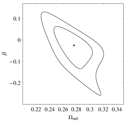
By minimizing the corresponding total in Eq. (18), we find the best-fit parameters and , whereas . In Fig. 1, we present the corresponding and confidence level contours in the plane. Obviously, the current observational data slightly prefer a negative . We are also interested to the fractional energy densities given in Eq. (28) and , the deceleration parameter given in Eq. (24), and the effective equation-of-state parameter (EoS) . We present them as functions of redshift with the best-fit model parameters in Fig. 2. It is easy to find the transition redshift where the universe changes from deceleration () to acceleration (). Since the best-fit is negative, dark matter decays into dark energy () when , and dark energy decays into dark matter () when . The interaction crosses the non-interacting line () at .


III.2 The case of
Secondly, we consider the case of given in Eq. (9). From Eq. (6), it is easy to find . Substituting into Eq. (9), we can finally obtain
| (32) |
Substituting Eqs. (21) and (32) into Eq. (1), we have
| (33) |
Similarly, we recast it as
| (34) |
which is a second-order differential equation for . Note that the deceleration parameter is also a function of and [cf. Eq. (24)]. Similar to the case of , we consider only the case of in this work. In this case, the sign-changeable interaction reads
| (35) |
By solving the second-order differential equation (34) with , we find that
| (36) |
where , are both integral constants, and
| (37) |
Substituting Eq. (36) into Eq. (27), we have
| (38) |
Requiring , we obtain
| (39) |
On the other hand, requiring , from Eq. (36) we can find that
| (40) |
From Eqs. (36) and (40), it is easy to obtain
| (41) |
where and have been given in Eqs. (39) and (37), respectively. There are two free model parameters, namely and . Note that when , Eq. (41) reduces to , i.e., the one of CDM model.
Imposing the condition when , we have from Eq. (38). Under this condition, by minimizing the corresponding total in Eq. (18), we find the best-fit parameters and , whereas . In Fig. 3, we present the corresponding and confidence level contours in the plane. In Fig. 4, we also present the given in Eq. (38), , given in Eq. (24) and as functions of redshift with the best-fit model parameters. The universe changes from deceleration () to acceleration () at the transition redshift .
However, the above best-fit model with is in fact the CDM model without interaction between dark energy and dark matter. So, we would like to give up the condition . This means that in the early universe we have and then , namely, might be negative. Since the negative energy density can arise in quantum field theory (see e.g. [28] for a good review), it is reasonable to consider this possibility. Without the condition , by minimizing the corresponding total in Eq. (18), we find the best-fit parameters and , whereas . In Fig. 5, we present the corresponding and confidence level contours in the plane. Obviously, the current observational data slightly prefer a negative . In Fig. 6, we also present the given in Eq. (38), , given in Eq. (24) and as functions of redshift with the best-fit model parameters. It is easy to find the transition redshift where the universe changes from deceleration () to acceleration (). Since the best-fit is negative, dark matter decays into dark energy () when , and dark energy decays into dark matter () when . The interaction crosses the non-interacting line () at .

III.3 The case of
Finally, we consider the case of given in Eq. (10). Substituting it into Eq. (5), one can find that
| (42) |
Then, substituting into Eq. (10), we can finally obtain
| (43) |
From Eqs. (6) and (7) [or equivalently Eq. (21)], we have
| (44) |
Substituting Eqs. (21), (43) and (44) into Eq. (1), we find that
| (45) |
Similarly, we recast it as
| (46) |
which is a second-order differential equation for . Note that the deceleration parameter is also a function of and [cf. Eq. (24)]. Unfortunately, if , there is no analytical solution for the second-order differential equation (46), because one will encounter a transcendental equation. Therefore, we consider only the case of in this work. In this case, the sign-changeable interaction reads
| (47) |
By solving the second-order differential equation (46) with , we find that
| (48) |
where , are both integral constants, and
| (49) |
Substituting Eq. (48) into Eq. (27), we have
| (50) |
Requiring , we obtain
| (51) |
On the other hand, requiring , from Eq. (48) we get
| (52) |
From Eqs. (48) and (52), it is easy to obtain
| (53) |
where and have been given in Eqs. (51) and (49), respectively. There are two free model parameters, namely and . Note that when , Eq. (53) reduces to , i.e., the one of CDM model.

By minimizing the corresponding total in Eq. (18), we find the best-fit parameters and , whereas . In Fig. 7, we present the corresponding and confidence level contours in the plane. Obviously, the current observational data slightly prefer a positive . In Fig. 8, we also present the given in Eq. (50), , given in Eq. (24) and as functions of redshift with the best-fit model parameters. It is easy to find the transition redshift where the universe changes from deceleration () to acceleration (). Since the best-fit is positive, dark energy decays into dark matter () when , dark matter decays into dark energy () when . The interaction crosses the non-interacting line () at .

IV Concluding remarks
Recently, Cai and Su [15] found that the sign of interaction in the dark sector changed in the approximate redshift range of , by using a model-independent method to deal with the observational data. In fact, this result raises a remarkable problem, since most of the familiar interactions cannot change their signs in the whole cosmic history. Motivated by the work of Cai and Su, we have proposed a new type of interaction in a previous work [16]. The key ingredient is the deceleration parameter in the interaction , and hence the interaction can change its sign when our universe changes from deceleration () to acceleration (). In the present work, we consider the cosmological constraints on this new type of sign-changeable interactions, by using the latest observational data. We find that the cosmological constraints on the model parameters are fairly tight. In particular, the key parameter has been constrained to a narrow range.
Some remarks are in order. Firstly, we briefly consider the comparison of these models. For convenience, we also consider the well-known CDM model in addition. In fact, it corresponds to the decaying model with . Fitting CDM model to the observational data considered in the present work, it is easy to find the corresponding best-fit parameter , whereas . Of course, we would like to also consider the decaying model with a traditional interaction which cannot change its sign in the whole cosmic history. The corresponding can be found in e.g. [12], namely
| (54) |
Fitting to the same observational data, we find the best-fit parameters and , whereas . A conventional criterion for model comparison in the literature is , in which the degree of freedom , whereas and are the number of data points and the number of free model parameters, respectively. We present the for all the 6 models in Table 1. On the other hand, there are other criterions for model comparison in the literature, such as Bayesian Information Criterion (BIC) and Akaike Information Criterion (AIC). The BIC is defined by [29, 31]
| (55) |
where is the maximum likelihood. In the Gaussian cases, . So, the difference in BIC between two models is given by . The AIC is defined by [30, 31]
| (56) |
The difference in AIC between two models is given by . In Table 1, we also present the BIC and AIC of all the 6 models considered in this work. Notice that CDM has been chosen to be the fiducial model when we calculate BIC and AIC. From Table 1, it is easy to see that the rank of models is coincident in all the 3 criterions (, BIC and AIC). The CDM model is still the best one. However, it is well known that CDM model is plagued with the cosmological constant problem and the coincidence problem (see e.g. [1]). On the other hand, there are some observational evidences for the interaction between dark energy and dark matter [13, 14], and the coincidence problem can be alleviated in the interacting dark energy models. Therefore, it is still worthwhile to study the interacting dark energy models. Although the model with traditional interaction (which cannot change its sign) is very close to the other models with sign-changeable interactions, the latter are phenomenally richer (see e.g. [16]). Therefore, we consider that the models with sign-changeable interactions deserve further investigations.
| Model | CDM | |||||
|---|---|---|---|---|---|---|
| () | with | without | ||||
| Best fit | ||||||
| 542.919 | 542.735 | 542.725 | 542.919 | 542.711 | 542.778 | |
| 1 | 2 | 2 | 2 | 2 | 2 | |
| 0.9730 | 0.9744 | 0.9744 | 0.9747 | 0.9743 | 0.9745 | |
| BIC | 0 | 6.142 | 6.132 | 6.326 | 6.118 | 6.185 |
| AIC | 0 | 1.816 | 1.806 | 2.0 | 1.792 | 1.859 |
| Rank | 1 | 4 | 3 | 6 | 2 | 5 |
Secondly, we note that the case of is fairly different from the cases of and . Comparing Fig. 7 with Figs. 1, 3 and 5, it is easy to see that the direction of contours in the plane is rightward for the case of , whereas the ones are leftward for the cases of and . From Table 1, we find that the best-fit is positive for the case of , whereas the ones are negative (or zero) for the cases of and . This means that in the case of the interaction crosses the non-interacting line () from above to below, whereas in the cases of and the interaction crosses the non-interacting line () from below to above. This is physically interesting, because means that the energy transfers from dark energy to dark matter, whereas means that the energy transfers from dark matter to dark energy.
Finally, in this work the role of dark energy is only played by the decaying (vacuum energy), whereas the parameter in the sign-changeable interactions are chosen to be zero. So, the constraints obtained in this work cannot be directly used to the models different from the ones considered here. In fact, the interacting dark energy models with sign-changeable interactions can be generalized. For instance, one can choose dark energy to be the one with a constant or variable EoS (including parameterized EoS, or even the ones of quintessence, phantom, k-essence, Chaplygin gas, quintom, hessence, holographic or agegraphic dark energy, and so on). Of course, one can also let the parameter be free and then constrain the models numerically.
ACKNOWLEDGEMENTS
We thank the referee for quite useful comments and suggestions, which help us to improve this work. We are grateful to Professors Rong-Gen Cai and Shuang Nan Zhang for helpful discussions. We also thank Minzi Feng, as well as Xiao-Peng Ma, for kind help and discussions. This work was supported in part by NSFC under Grant No. 10905005, the Excellent Young Scholars Research Fund of Beijing Institute of Technology, and the Fundamental Research Fund of Beijing Institute of Technology.
References
- [1]
E. J. Copeland, M. Sami and S. Tsujikawa,
Int. J. Mod. Phys. D 15, 1753 (2006) [hep-th/0603057];
J. Frieman, M. Turner and D. Huterer, Ann. Rev. Astron. Astrophys. 46, 385 (2008) [arXiv:0803.0982]. - [2] E. J. Copeland, A. R. Liddle and D. Wands, Phys. Rev. D 57, 4686 (1998) [gr-qc/9711068].
- [3]
Z. K. Guo, R. G. Cai and Y. Z. Zhang,
JCAP 0505, 002 (2005) [astro-ph/0412624];
Z. K. Guo, Y. S. Piao, X. M. Zhang and Y. Z. Zhang, Phys. Lett. B 608, 177 (2005) [astro-ph/0410654];
Z. K. Guo, N. Ohta and S. Tsujikawa, Phys. Rev. D 76, 023508 (2007) [astro-ph/0702015]. - [4]
L. Amendola,
Phys. Rev. D 60, 043501 (1999) [astro-ph/9904120];
L. Amendola, Phys. Rev. D 62, 043511 (2000) [astro-ph/9908023];
L. Amendola and C. Quercellini, Phys. Rev. D 68, 023514 (2003) [astro-ph/0303228];
L. Amendola and D. Tocchini-Valentini, Phys. Rev. D 64, 043509 (2001) [astro-ph/0011243];
L. Amendola and D. Tocchini-Valentini, Phys. Rev. D 66, 043528 (2002) [astro-ph/0111535];
L. Amendola et al., Astrophys. J. 583, L53 (2003) [astro-ph/0205097]. - [5]
T. Damour and A. M. Polyakov,
Nucl. Phys. B 423, 532 (1994) [hep-th/9401069];
T. Damour and A. M. Polyakov, Gen. Rel. Grav. 26, 1171 (1994) [gr-qc/9411069];
C. Wetterich, Astron. Astrophys. 301, 321 (1995) [hep-th/9408025];
J. R. Ellis, S. Kalara, K. A. Olive and C. Wetterich, Phys. Lett. B 228, 264 (1989);
G. Huey, P. J. Steinhardt, B. A. Ovrut and D. Waldram, Phys. Lett. B 476, 379 (2000) [hep-th/0001112];
C. T. Hill and G. G. Ross, Nucl. Phys. B 311, 253 (1988);
G. W. Anderson and S. M. Carroll, astro-ph/9711288;
B. Gumjudpai, T. Naskar, M. Sami and S. Tsujikawa, JCAP 0506, 007 (2005) [hep-th/0502191]. - [6]
H. Wei and R. G. Cai,
Phys. Rev. D 71, 043504 (2005) [hep-th/0412045];
H. Wei and R. G. Cai, Phys. Rev. D 72, 123507 (2005) [astro-ph/0509328];
H. Wei and S. N. Zhang, Phys. Rev. D 76, 063005 (2007) [arXiv:0705.4002];
H. Wei, N. N. Tang and S. N. Zhang, Phys. Rev. D 75, 043009 (2007) [astro-ph/0612746];
H. Wei and R. G. Cai, Phys. Rev. D 73, 083002 (2006) [astro-ph/0603052];
H. Wei and R. G. Cai, JCAP 0709, 015 (2007) [astro-ph/0607064];
H. Wei, Phys. Lett. B 695, 307 (2011) [arXiv:1002.4230]. - [7]
W. Zimdahl and D. Pavon,
Phys. Lett. B 521, 133 (2001) [astro-ph/0105479];
L. P. Chimento, A. S. Jakubi, D. Pavon and W. Zimdahl, Phys. Rev. D 67, 083513 (2003) [astro-ph/0303145]. - [8]
R. G. Cai and A. Wang,
JCAP 0503, 002 (2005) [hep-th/0411025];
E. Majerotto, D. Sapone and L. Amendola, astro-ph/0410543. - [9] X. M. Chen, Y. G. Gong and E. N. Saridakis, JCAP 0904, 001 (2009) [arXiv:0812.1117].
- [10]
L. P. Chimento,
Phys. Rev. D 81, 043525 (2010) [arXiv:0911.5687];
L. P. Chimento, M. Forte and G. M. Kremer, Gen. Rel. Grav. 41, 1125 (2009) [arXiv:0711.2646]. - [11]
J. H. He, B. Wang and Y. P. Jing,
JCAP 0907, 030 (2009) [arXiv:0902.0660];
J. H. He, B. Wang and P. Zhang, Phys. Rev. D 80, 063530 (2009) [arXiv:0906.0677];
J. H. He, B. Wang, E. Abdalla and D. Pavon, JCAP 1012, 022 (2010) [arXiv:1001.0079]. - [12] H. Wei and S. N. Zhang, Phys. Lett. B 644, 7 (2007) [astro-ph/0609597].
- [13]
O. Bertolami, F. Gil Pedro and M. Le Delliou,
Phys. Lett. B 654, 165 (2007) [astro-ph/0703462];
O. Bertolami, F. G. Pedro and M. Le Delliou, Gen. Rel. Grav. 41, 2839 (2009) [arXiv:0705.3118];
M. Le Delliou, O. Bertolami and F. Gil Pedro, AIP Conf. Proc. 957, 421 (2007) [arXiv:0709.2505];
O. Bertolami, F. G. Pedro and M. L. Delliou, arXiv:0801.0201 [astro-ph]. - [14]
E. Abdalla, L. R. Abramo, L. Sodre and B. Wang,
Phys. Lett. B 673, 107 (2009) [arXiv:0710.1198];
E. Abdalla, L. R. Abramo and J. C. C. de Souza, Phys. Rev. D 82, 023508 (2010) [arXiv:0910.5236]. - [15] R. G. Cai and Q. P. Su, Phys. Rev. D 81, 103514 (2010) [arXiv:0912.1943].
- [16] H. Wei, Nucl. Phys. B 845, 381 (2011) [arXiv:1008.4968].
- [17]
P. Wang and X. H. Meng,
Class. Quant. Grav. 22, 283 (2005) [astro-ph/0408495];
F. E. M. Costa and J. S. Alcaniz, Phys. Rev. D 81, 043506 (2010) [arXiv:0908.4251]. - [18]
R. Amanullah et al. [SCP Collaboration],
Astrophys. J. 716, 712 (2010) [arXiv:1004.1711].
The numerical data of the full Union2 sample are available at http:supernova.lbl.gov/Union - [19] E. Komatsu et al. [WMAP Collaboration], Astrophys. J. Suppl. 192, 18 (2011) [arXiv:1001.4538].
- [20]
M. Tegmark et al. [SDSS Collaboration],
Phys. Rev. D 69, 103501 (2004) [astro-ph/0310723];
M. Tegmark et al. [SDSS Collaboration], Astrophys. J. 606, 702 (2004) [astro-ph/0310725];
U. Seljak et al. [SDSS Collaboration], Phys. Rev. D 71, 103515 (2005) [astro-ph/0407372];
M. Tegmark et al. [SDSS Collaboration], Phys. Rev. D 74, 123507 (2006) [astro-ph/0608632]. - [21] D. J. Eisenstein et al. [SDSS Collaboration], Astrophys. J. 633, 560 (2005) [astro-ph/0501171].
- [22]
S. Nesseris and L. Perivolaropoulos,
Phys. Rev. D 72, 123519 (2005) [astro-ph/0511040];
L. Perivolaropoulos, Phys. Rev. D 71, 063503 (2005) [astro-ph/0412308]. - [23] E. Di Pietro and J. F. Claeskens, Mon. Not. Roy. Astron. Soc. 341, 1299 (2003) [astro-ph/0207332].
- [24] Y. Wang and P. Mukherjee, Astrophys. J. 650, 1 (2006) [astro-ph/0604051].
- [25] J. R. Bond, G. Efstathiou and M. Tegmark, Mon. Not. Roy. Astron. Soc. 291, L33 (1997) [astro-ph/9702100].
- [26] S. Nesseris and L. Perivolaropoulos, Phys. Rev. D 70, 043531 (2004) [astro-ph/0401556].
- [27]
H. Wei,
Eur. Phys. J. C 60, 449 (2009) [arXiv:0809.0057];
H. Wei, Phys. Lett. B 691, 173 (2010) [arXiv:1004.0492]. - [28]
L. H. Ford,
Int. J. Mod. Phys. A 25, 2355 (2010) [arXiv:0911.3597].
However, it is worth noting that the negative dark energy density considered here differs from the one in the above reference, because it is local in quantum field theory. In fact, the energy density of a component can be negative as long as total energy remains positive, as discussed in [32] (we thank the referee for pointing out this issue). - [29] G. Schwarz, Ann. Stat. 6, 461 (1978).
- [30] H. Akaike, IEEE Trans. Automatic Control 19, 716 (1974).
- [31]
M. Li, X. D. Li and X. Zhang,
Sci. China Phys. Mech. Astron. 53, 1631 (2010)
[arXiv:0912.3988];
H. Wei, JCAP 1008, 020 (2010) [arXiv:1004.4951]. - [32] Z. K. Guo, Y. S. Piao, X. M. Zhang and Y. Z. Zhang, Phys. Rev. D 74, 127304 (2006) [astro-ph/0608165].