On Vector Meson Masses in a Holographic SQCD

The gauge/string correspondence and its numerous generalizations (see [1] for a review) conjectures the equivalence between (super)string theory on a ten-dimensional space-time and some gauge theory living on the boundary of this space-time. The approach is based on taking the near horizon limit of the background produced by a large number of $Dp$-branes. On the field theory side the number of branes $N_{c}$ corresponds to the rank of the gauge group(s). Therefore the gauge/string correspondence provides a holographic description of the field theory in the planar limit. Large $N_{c}$ and supersymmetry contribute to the differences between the holographic models and the real world QCD. Yet, for many phenomenological applications the holographic approach can provide a valuable insight. In the holographic approach, in order to add a meson sector one has to include “flavor” D-branes [2], giving rise to the quark degrees of freedom. Such models, colloquially called holographic QCD, have been extensively studied over the last decade for various gravity backgrounds with different flavor D-branes.

We choose the Klebanov-Strassler (KS) [3] background as the starting point for our holographic setup. This background is dual to a confining supersymmetric gauge theory which cascades to a $\mathcal{N}=1$ $SU(M)$ SYM in the deep IR. On the gravity side the KS solution is based on the $6d$ deformed conifold. The deformation parameter $\epsilon$ is related to the dynamical scale $\Lambda$ of the gauge theory. Apart from $\Lambda$, the real life QCD also includes additional massive parameters – the quark masses $m_{\rm q}$. In this paper we will focus on a holomorphic $D7$-brane previously studied in [4]. For the sake of simplicity, we will consider a single $D7$-brane. Thus we can use the quenched approximation ignoring the backreaction of the flavor brane on the gravity background. In general, the approximation is valid for $N_{\rm f}\ll N_{\rm c}$. The holomorphicity of the embedding implies that it breaks none of the background supersymmetries and the dual gauge theory with flavor is a $\mathcal{N}=1$ SYM with fundamental matter. The embedding of the $D7$-brane is parametrized by a single complex parameter $\mu$ which is related to the quark mass. The preserved supersymmetry allows us to write down the precise form of the superpotential. It appears that apart from the quark mass term there is a term describing quartic interaction between the quarks and the KS bi-fundamentals.

The low energy fields living on the $D7$-brane are the complex scalar that corresponds to the directions transversal to the brane and the $8d$ gauge field. From the $4d$ point of view the latter decomposes into a gauge field and another three real scalars. The gauge field is dual to the conserved $U(1)_{\rm f}$ flavor symmetry current that gives rise to the vector mesons. All other fields are dual to scalar operators related to each other by supersymmetry. We review the meson multiplet structure later in the text. Although the calculation of the scalar meson spectrum currently appears to be a hard technical problem, the vector meson spectrum can be computed relatively easy for any value of $\mu/\epsilon$. We thus have a remarkable opportunity to investigate how the vector meson mass $m$ depends on both the quark mass $m_{\rm q}$ and the IR scale $\Lambda$, with the former fixed by $\mu$ and the latter by $\epsilon$.

It is worth recalling here that we are dealing with a supersymmetric version of QCD and as a result both $\Lambda$ and $m_{\rm q}$ ($\epsilon$ and $\mu$) are complex parameters. Naively, for a fixed $\epsilon$, the meson masses are expected to grow as we increase $|\mu|$: the meson built of heavier quarks is supposed to be heavier. Surprisingly, we found numerically that this is not the case if the ratio $x\equiv\mu/\epsilon$ is real and smaller than a certain value, approximately equal to one. In this case only the lowest meson behaves as expected, i.e. its mass increases with $x$. At the same time the masses of all other modes decrease as $x$ increases from $0$ to $1$. Then, around $x\approx 1$ the masses reach their minimum and increase afterwards. This is an unusual behavior both because the meson mass is not a monotonic function of $\mu$ and because it singles out the lowest mode. To confirm the result of numerics we use the WKB analysis reaching the same conclusion.

In Nature the lightest vector mesons are the $\rho$-mesons built from the $u$ and $d$ quarks. These quarks are much lighter than the QCD scale. We compared the ratio of the lowest $\rho$-meson masses with the predictions of our model for $\mu=0$ and found a remarkably good agreement assuming that the $\rho(2150)$ meson is a $3\,^{3}S_{1}$ mode.¹¹ 1 The experimental status of the $3\,^{3}S_{1}$ mode is presently unclear. We discuss this issue later in the text.

Next in the spectrum of vector mesons after the $\rho$’s are the $\phi$-mesons built from the heavier $s$ and $\overline{s}$ quarks. These mesons, however, can mix the “pure” $s\overline{s}$ states with $u\overline{u}$ and $d\overline{d}$. To compare with the holographic model we use putative pure “$\phi$”-mesons, whose masses can be derived from the spectrum of the $K^{\star}$ and $\rho$-mesons. We found similarity between the non-monotonic behavior of the spectrum as a function of $x$ in our model and the putative “$\phi$”-meson masses. Namely the first excited mode of the “$\phi$”-meson (that consists of the heavy $s$-quarks) is lighter than the first excited mode of the $\rho$-meson (that consists of the light $u,d$-quarks). Remarkably, this applies only for the excited but not to the lowest mode, similarly to what we observed in our holographic model.

These optimistic results should not be taken for granted since our model is only a distinct relative of the real-world QCD. Nevertheless, we believe that the observed similarities may not be a mere coincidence. It can rather suggest that the ratio of masses for certain light excitations in the QCD-like theories is quite robust and is not sensitive neither to the number of colors, nor to the explicit field content of the field theory. A similar phenomenon was previously observed for certain glueballs: the KS theory happens to predict with a reasonable accuracy the mass ratio for the lightest scalar glueballs of the pure $SU(3)$ theory [5].

As another option, it may be the case that the inverse mass phenomenon is actually a result of some peculiarities of our model, not shared by QCD. Thus the quartic interaction between the quarks and the original fields of the KS model may provide a nice intuitive explanation for the different spectrum behavior for real and pure imaginary $\mu$. This argument has also a clear geometrical counterpart. In terms of the dual geometry, the minimal distance between the tip of the deformed conifold and the lowest point on the ${\rm D}7$-brane depends on $x$ in an interesting way. When $x$ has a non-zero phase the distance vanishes only for $x=0$, while for real $x$ the brane extends all the way to the tip as long as $0\leqslant x\leqslant 1$. Hence we have different behavior for real and complex $x$.

The deformed conifold is a regular six dimensional non-compact CY manifold defined by the equation

The relevant $10d$ supergravity solution is of the GKP type [6] with constant dilaton and a warped metric

Here $ds_{6}^{2}$ is the (deformed) conifold metric and the warp-factor $h(r)$ depends on the transverse radial variable $r$ defined by

The minimal value of $r$ is $r=|\epsilon|^{2/3}$ and in the deformed conifold case it is useful to introduce a new coordinate $\tau$ defined by

We refer the reader to the original paper [3] for the explicit form of the deformed conifold metric, fluxes and the warp factor.

The field theory dual of the singular ($\epsilon=0$) conifold background is a ${\cal N}=1$ $4d$ gauge theory at an IR conformal point, known as the Klebanov-Witten (KW) theory [7]. For the deformed conifold ($\epsilon\neq 0$) the gauge group is $SU\left((k+1)M\right)\times SU(kM)$ for integer $k$. The shift $k\to k-1$ describes a single step in a cascade of Seiberg dualities, which reduces the gauge group down to $SU(2M)\times SU(M)$ in the deep IR. The R-symmetry is broken down to ${\mathbb{Z}}_{2}$ due to the formation of a gluino condensate $\langle\lambda\lambda\rangle\sim\Lambda^{3}$. On the gravity side the scale $\Lambda$ is fixed by the conifold deformation parameter $\epsilon$.

At the next step we consider a $D7$-brane embedded in the KS background. The $D7$-brane extends along the flat Minkowski space-time and a holomorphic non compact four cycle on the conifold $\Sigma$. The embedding we are interested in is

It was shown in [4] that the $D7$-brane wrapping $\Sigma$ with trivial world-volume gauge field does not break the $\mathcal{N}=1$ SUSY of the original theory. Moreover, the $4$-cycle wrapped by the brane is topologically trivial [4, 8], thus the tadpole cancellation condition is satisfied and no anti $D7$-brane is required in order cancel the net RR charge. On the gauge theory side it implies that the setup has no chiral symmetry. This is in contrast to the conifold based model of [8, 9] (see also [10, 11]).

The lowest value of the radial coordinate $\tau_{\rm min}$ along the profile depends on the relative phase between $\mu$ and $\epsilon$. A simple computation shows that

where

This means that for real $x$ we have $\tau_{\rm min}=0$ as long as $|x|\leqslant 1$. On the other hand, if $x$ has a non-zero imaginary part, then necessarily $\tau_{\rm min}>0$. For fixed $\tau$ the geometry of $\Sigma$ is $S^{3}/\mathbb{Z}_{2}$ which shrinks to $S^{2}$ at $\tau=\tau_{\rm min}$.

The quiver diagram for the flavored Klebanov-Witten model is shown on Figure 1 and the superpotential is [12, 13, 14]

where $A_{1,2}$, $B_{1,2}$ are bi-fundamental matter fields. Thus the term $2\mu\tilde{q}q$ is responsible for the quark mass.

The right degrees of freedom for a confining theory are the di-baryon operators $\mathcal{A}$ and $\mathcal{B}$ constructed from the bi-fundamentals or mesonic operators of the form ${\rm Tr}\left(A_{i}B_{j}\right)$. One of the striking features of the KS model is that the superpotential retains its form under Seiberg duality. The KS solution describes an $\mathcal{A}\leftrightarrow\mathcal{B}$-symmetric point in the baryonic branch, which is evident, in particular, from the additional un-broken $\mathbb{Z}_{2}$ symmetry of the background.

Let us now address the map between various fields on the $D7$-brane and the gauge theory states.

As we have already mentioned in the Introduction, the world-volume fields on the flavor $D7$-brane are a complex scalar $\delta\mu$ and a $8d$ gauge field $a_{M}$. Throughout this paper we will adopt the $a_{\tau}=0$ gauge. This leaves the $4d$ $a_{\mu}$ components and the $a_{i}$ legs along $\Sigma$ at finite $\tau$. The KS background describes a confining theory and only the colorless combinations of the quarks fields, like the mesons $q\tilde{q}$, appear in the spectrum. Both $q$ and $\tilde{q}$ are $4d$ chiral multiplets. The bottom component of the operator $\tilde{q}q$ has dimension $3/2$. This is evident from the superpotential (8). This operator corresponds to the combination $a_{1}+ia_{2}$. The top component $\int d^{2}\theta\ q\tilde{q}$ has dimension $5/2$ and corresponds to the complex scalar describing the embedding. Furthermore, the world-volume gauge field with space-time indexes $a_{\mu}$ is dual to the $U(1)_{\rm f}$ vector current $J_{\mu}$, and the remaining component of the world-volume gauge field $a_{3}$ is dual to the bottom component of the $U(1)_{\rm f}$ current multiplet.

In the holographic approach the $4d$ mesons arise as the normalizable fluctuations of the $D7$-brane world-volume fields. The $\mathcal{N}=1$ SUSY arranges the particles into multiplets combining a massive vector with a real scalar or two real scalars together (we are not concerned with fermions here). There are no massless mesons in the setup in question. As was mentioned above the supersymmetry combines the vector mesons (the focus of this publication) with the scalars originating from the fluctuation of the world-volume gauge field $a_{3}$. Although these particles have the same spectrum the equations they obey in the bulk are not the same. Rather they are related to each other through a supersymmetric quantum mechanics (SUSY QM) transformation [15]. This situation is typical for the fluctuations that are dual to operators of different dimension. The equations for different particles in the multiplet coincide only if the corresponding dual operators are of the same dimension. In the present case the vector current has dimension 3 and the bottom component of the current multiplet has dimension 2, and therefore only the related spectra will coincide but not the equations themselves. The SUSY QM transformation also relates the pair of scalars originating from the fluctuations of the world-volume gauge field $a_{1,2}$ and the fluctuations of the embedding $\mbox{Re}\ \delta\mu,\mbox{Im}\ \delta\mu$. Since $a_{1,2}$ correspond to the operators of dimension $3/2<2$, to find the spectrum one has to impose the “unusual” boundary conditions at infinity [16]. While the general asymptotic of $a_{1,2}$ is $c_{0}r^{-1/2}+c_{1}r^{-3/2}$, the proper boundary conditions for $a_{1,2}$ are $c_{1}=0$ with arbitrary $c_{0}$. In practice this would mean that to obtain the spectrum from the original equations for $a_{1,2}$ in the bulk, using (for example) the shooting technique, may not be the optimal strategy. Rather one can study the equations for the superpartners $\mbox{Re}\ \delta\mu,\mbox{Im}\ \delta\mu$ which yield the same spectrum. These fluctuations correspond to the operators of dimension $5/2>2$ and although they have the same (up to an overall $r^{-1/2}$ factor) asymptotic at infinity $c_{0}+c_{1}r^{-1}$, they satisfy the conventional boundary conditions $c_{0}=0$ with arbitrary $c_{1}$. It happens that in the conformal KW case there is an accidental degeneracy between $a_{1}$ and $a_{2}$ (as well as between $\mbox{Re}\ \delta\mu$ and $\mbox{Im}\ \delta\mu$) [15]. It will be interesting to see if this degeneracy will be lifted in the KS case when the new parameter $\epsilon$ is introduced.

In this section we will calculate the spectrum of the vector mesons as a function of $\mu,\epsilon$. These mesons are created by the $U(1)_{\rm f}$ flavor current $J_{\mu}$ dual to the Minkowskian vector field living on the $D7$-brane. The five-dimensional action describing the lowest KK modes of this vector field has the form

Here $\mu,\nu$ are the Minkowski indexes and $\tau$ is the radial direction along the conifold. We choose the gauge $a_{\tau}=0$ and look for a solution of the form $a_{\mu}=v_{\mu}e^{ik\cdot x}\psi(\tau)$ with $v\cdot k=0$ and

The four-dimensional meson mass $m^{2}=-k^{2}$ emerges from the eigenvalue problem (10). In general, to find the functions $C(\tau)$ and $D(\tau)$ could be a tiresome task. This is because both the DBI and the CS parts of the $D7$-brane action contribute to the action (9). The problem drastically simplifies for a SUSY $D7$-brane embedded into a constant dilaton, imaginary self-dual (ISD) background [9]. In this case the invariant 2-form $\mathcal{F}\equiv\varphi^{\star}(B_{2})+2\pi\alpha^{\prime}dA$, where $\varphi^{\star}$ denotes the pull-back, satisfies the anti-self-duality condition

which implies [9]

Here $g$ stands for the un-warped induced metric on the 4-cycle $\Sigma$ wrapped by the $D7$-brane and $\star_{4}$ is the Hodge dual associated with $g$. The equation (11) follows directly from the $\kappa$-symmetry condition, which in turn ensures that the embedding preserves the background supersymmetry. It was shown in [4] that the $B$-field in the original gauge of the KS solution fulfills the $\kappa$-symmetry condition with zero world-volume gauge field $A=0$. Hence in what follows we can substitute $\mathcal{F}$ with $B$ assuming the pullback on $\Sigma$.

As a result we find for our embedding

and the KS warp factor is

Here $m_{\rm gb}$ is the scale mass of the gauge theory glueballs

and $x$ is the complex dimensionless parameter defined above

To derive the first expression in (13) one has to introduce a complete set of local coordinates on $\Sigma$, for example as it was done in [17]. The last two relations easily follow from the explicit form of the Kähler form and the NS flux on the deformed conifold as well as the relations between different forms on $\Sigma$ [18].

The mode $\psi$ from (10) is dual to an operator of dimension 3, a fact which is in agreement with its asymptotic behavior at infinity²² 2 Notice that at infinity $r^{3}\approx\frac{1}{2}\left|\epsilon\right|^{2}e^{\tau}$.

The proper boundary conditions are $c_{0}=0$, i.e. $\displaystyle{\lim_{\tau\to\infty}\psi(\tau)=0}$ at infinity, and regularity at the origin $\tau=\tau_{\rm min}$, where $\psi\approx 1+d_{2}(\tau-\tau_{\rm min})^{2}$ with a numerical coefficient $d_{2}=d_{2}(x,m/m_{\rm gb})$. These boundary conditions represent no challenge for numerical studies of the spectrum and the equation (10) can be solved with a standard shooting technique. What we actually calculate in this way is the ratio $m/m_{\rm gb}$ between the meson and the glueball masses as a function of $x$. Since the glueball mass $m_{\rm gb}$ is $\mu$ independent, changing $x$ is equivalent to changing $\mu$, while keeping $\epsilon$ fixed.

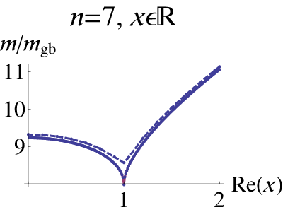
We solved (10) numerically for various values of $x$. Because the spectrum is invariant under $x\rightarrow-x$ and $x\rightarrow x^{*}$ we focused only on the $\mbox{Re}\ x,\mbox{Im}\ x>0$ quadrant. In Table 1 we present our results³³ 3 The mass values for $x=0$ are different from those in [4] due to numerical errors therein. for $x=0$ and some real and purely imaginary values of $x$. As one can see, if $x$ is real, for all modes, except for the lowest one, the meson masses decrease as $x$ grows, until they reach their minimum value around $x\approx 1$. Then they start growing again. This type of behavior is not observed for the purely imaginary values of $x$, for which the masses grow monotonically with $|x|$. The results are presented graphically on Figures 2, 3. Our analysis seems then to imply that, for real $x$ smaller than $1$, the higher level mesons composed of heavier quarks are actually lighter than those composed of lighter quarks.

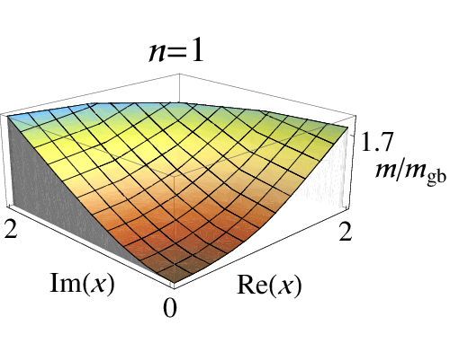
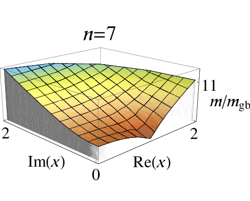
This surprising behavior is confirmed by the WKB analysis, performed along the lines of [19] (as reported in Appendix B of [20]). After putting equation (10) in the Schrödinger form

one can use the standard WKB formula

Here $\tau^{*}$ is the point where the potential vanishes, $V(\tau^{*})=0$. For larger $m$ this happens at larger $\tau$ where $V(\tau)$ can be approximated by

Thus $\tau^{*}$ is very large for large $m$ and is $x$-independent. Hence we simply substitute it by infinity. In the large $m$ limit we therefore have

In Figure 3 we plot the meson masses calculated for real (left) and imaginary (right) $x$ for the excited mode $n=7$; the bottom solid line is the WKB result, while the upper dashed line is the result of the shooting. The strange behavior found for real $x$ with the shooting technique is perfectly reproduced by the WKB approximation.

A similar behavior was found in the model studied in [21] (Figure 4). It is worth emphasizing that also in that model the bare quark mass can be tuned to be smaller than the dynamical generated scale. This is definitely not a common feature in holographyc models. For example, in the original Sakai-Sugimoto model [22] it is unclear how to tune the bare mass (the distance of the flavor branes from the tip of the cigar just reflecting variations of the constituent mass). In this sense, the KS background provides a privileged environment for the study of flavors with non-zero bare mass.

We can derive the strange behavior of the excited ($n>1$) modes for real $x$ directly from the form of $\Theta(\tau)$ in (21). In the interval $0\leqslant x<1$ we have $\tau_{\rm min}=0$ and the function $\Theta(\tau,x)$ has the same asymptotic values at the origin $\Theta(0,x)=2^{-5/3}3^{-1/3}I(0)$ and infinity $\displaystyle{\lim_{\tau\to\infty}}\Theta(\tau,x)=0$, but it monotonically increases with $x$ for any $\tau$ in between zero and infinity as demonstrated on the left graph on Figure 4. Hence the integral $\Delta(x)$ is a monotonically decreasing function with $x$, as expected. At $x=1$ the asymptotic value of $\Theta(\tau,x)$ at the origin $\tau=0$ jumps to $\Theta(0,1)=2^{-2/3}3^{-1/3}I(0)$ but $\Delta(x)$ is continuous. For $x>1$ the asymptotic behavior of $\Theta(\tau,x)$ changes drastically: it blows at $\tau=\tau_{\rm min}$ as $\left(\tau-\tau_{\rm min}\right)^{-1}$. It is clear though that for $x$ very close to $1$ the behavior of $\Theta(\tau,x)$ as a function of $\tau$ will be the same as for $x=1$ except for some very small vicinity of $\tau=\tau_{\rm min}$. Hence the integral $\Delta(x)$ is a continuous function of $x$ as is expected from the physics of the problem. On the right graph on Figure 4 we adjusted the minimal value of the coordinate $\tau$ to the origin, $\tilde{\tau}\equiv\tau-\tau_{\rm min}$. It is clear now that as $x$ increases the function $\Theta(\tilde{\tau},x)$ decreases at each $\tilde{\tau}$. Therefore $\Delta(x)$ is monotonically decreasing with $x$ when $x\sim 1$. As a result we find that $\Delta(x)$ reaches its maximum, and the masses of the excited modes reach their minimum, at $x=1$. This is close to the numerical results in Table 1, where the lowest masses of the excited modes appear around $x=0.9$. It is worth mentioning here that the discussion in this paragraph is based on the WKB approximation which is usually not valid for small $n$, especially for $n=1$, and so the monotonic behavior of the lowest mode cannot be addressed in this framework.

The WKB analysis can also help us to see how the $\epsilon$ dependence disappears in the KW limit when $x\gg 1$. Indeed in this case we expect the meson mass to depend only on $\mu$ and hence to be proportional to $m_{\rm gb}|x|^{2/3}$. Such a behavior readily follows from (21). $\Theta(\tau,x)$ goes as $e^{-2\tau/3}$ for large $\tau$ and in order to find $\Delta(x)$ we need to integrate the square root of $\Theta(\tau,x)$ from $\tau_{\rm min}$ to infinity. For large $|x|$ the parameter $\tau_{\rm min}$ is also large and can be approximated by $e^{\tau_{\rm min}}\approx 4|x|^{2}$ as follows from (6). Putting all together we find $\Delta(x)$ to be proportional to $|x|^{-2/3}$ and therefore according to (21) we get $m_{n}\approx m_{\rm gb}|x|^{2/3}n$ as expected.

In this section we compare our results with the spectrum of the $\rho$ and $\phi$ mesons, i.e. the light quark $1^{--}$ vector mesons in QCD.⁴⁴ 4 The heavy quark $1^{--}$ mesons are not tightly bound in QCD, so the comparison with our values would be pointless. Before proceeding let us recall that the correspondence

is not rigorous. We just assume that the constant of proportionality is of the same order in the both cases. Similarly to $\epsilon$, the power of $\mu$ here follows merely from dimensional analysis.

Throughout this section we will use the standard $n^{2s+1}l_{j}$ notations for the $q\overline{q}$ mesons [25]. Here $n$ stands for the radial excitation number, $s$ is either $0$ (anti-parallel quark spins) or $1$ (parallel quark spins), and $l$ is the relative angular momentum of the quarks inside the meson. The latter is usually denoted by the conventional notations $S$, $P$, $D$, $\ldots$ for $l=0,1,2,\ldots$ Finally, $|l-s|\leqslant j\leqslant l+s$ is the total angular momentum of the state. An additional notation for the mesons is $j^{PC}$, where $P$ and $C$ are the parity and the charge conjugation respectively. In terms of $l$ and $s$ one has $P=(-1)^{l+1}$ and $C=(-1)^{l+s}$, and so the $S$-wave ($l=0$) $\rho$-mesons, that we study in this paper, have $1^{--}$ quantum numbers.

We are grateful to Francesco Bigazzi for collaboration on the early stages of this project. It is a pleasure to thank E. Klempt, J. Maldacena, D. Melnikov, A. Paredes and J. Soto for useful discussions, and J. Sonnenschein for his comments on the final version of the manuscript. We are grateful to E. Kiritsis for correspondence regarding the $\rho$-meson spectrum.

A.D. thanks the theory group at Vrije University Brussel for hospitality while this work was initiated. The research of A.D. was supported by the Stanford Institute for Theoretical Physics, by the DOE grant DE-FG02-90ER40542, by the Monell Foundation, and in part by the grant RFBR 07-02-00878 and the Grant for Support of Scientific Schools NSh- 3035.2008.2.

The work of S. K. is supported by the European Commission Marie Curie Fellowship under the contract IEF-2008-237488.

The research leading to the results in this paper has received funding from the European Community’s Seventh Framework Programme (FP7/2007-2013 under grant agreement n. 253534). This work is also supported by the FWO -Vlaanderen, project G.0235.05 and by the Federal Office for Scientific, Technical and Cultural Affairs through the Interuniversity Attraction Poles Programme (Belgian Science Policy) P6/11-P.

A. L. C. would like to thank the Italian students, parents, teachers and scientists for their activity in support of public education and research.

References

- [1] F. Bigazzi, A. L. Cotrone, M. Petrini, and A. Zaffaroni, “Supergravity duals of supersymmetric four dimensional gauge theories,” Riv. Nuovo Cim. 25N12 (2002) 1–70, hep-th/0303191.
- [2] A. Karch and E. Katz, “Adding flavor to AdS/CFT,” JHEP 06 (2002) 043, hep-th/0205236.
- [3] I. R. Klebanov and M. J. Strassler, “Supergravity and a confining gauge theory: Duality cascades and chiSB-resolution of naked singularities,” JHEP 08 (2000) 052, hep-th/0007191.
- [4] S. Kuperstein, “Meson spectroscopy from holomorphic probes on the warped deformed conifold,” JHEP 03 (2005) 014, hep-th/0411097.
- [5] A. Dymarsky, D. Melnikov, and A. Solovyov, “I-odd sector of the Klebanov-Strassler theory,” JHEP 05 (2009) 105, 0810.5666.
- [6] S. B. Giddings, S. Kachru, and J. Polchinski, “Hierarchies from fluxes in string compactifications,” Phys. Rev. D66 (2002) 106006, hep-th/0105097.
- [7] I. R. Klebanov and E. Witten, “Superconformal field theory on threebranes at a Calabi-Yau singularity,” Nucl. Phys. B536 (1998) 199–218, hep-th/9807080.
- [8] S. Kuperstein and J. Sonnenschein, “A New Holographic Model of Chiral Symmetry Breaking,” JHEP 09 (2008) 012, 0807.2897.
- [9] A. Dymarsky, S. Kuperstein, and J. Sonnenschein, “Chiral Symmetry Breaking with non-SUSY D7-branes in ISD backgrounds,” JHEP 08 (2009) 005, 0904.0988.
- [10] C. A. B. Bayona, H. Boschi-Filho, M. Ihl, and M. A. C. Torres, “Pion and Vector Meson Form Factors in the Kuperstein- Sonnenschein holographic model,” JHEP 08 (2010) 122, 1006.2363.
- [11] M. Ihl, M. A. C. Torres, H. Boschi-Filho, and C. A. B. Bayona, “Scalar and vector meson spectra of flavor chiral symmetry breaking in the Klebanov-Strassler background,” 1010.0993.
- [12] P. Ouyang, “Holomorphic D7-branes and flavored N = 1 gauge theories,” Nucl. Phys. B699 (2004) 207–225, hep-th/0311084.
- [13] F. Bigazzi, A. L. Cotrone, and A. Paredes, “Klebanov-Witten theory with massive dynamical flavors,” JHEP 09 (2008) 048, 0807.0298.
- [14] F. Bigazzi, A. L. Cotrone, A. Paredes, and A. Ramallo, “Non chiral dynamical flavors and screening on the conifold,” Fortsch. Phys. 57 (2009) 514–520, 0810.5220.
- [15] F. Benini and A. Dymarsky; in progress.
- [16] I. R. Klebanov and E. Witten, “AdS/CFT correspondence and symmetry breaking,” Nucl. Phys. B556 (1999) 89–114, hep-th/9905104.
- [17] F. Benini et. al., “Holographic Gauge Mediation,” JHEP 12 (2009) 031, 0903.0619.
- [18] A. Dymarsky, “Flavor brane on the baryonic branch of moduli space,” JHEP 03 (2010) 067, 0909.3083.
- [19] J. G. Russo and K. Sfetsos, “Rotating D3 branes and QCD in three dimensions,” Adv. Theor. Math. Phys. 3 (1999) 131–146, hep-th/9901056.
- [20] F. Bigazzi, A. L. Cotrone, A. Paredes, and A. V. Ramallo, “Screening effects on meson masses from holography,” JHEP 05 (2009) 034, 0903.4747.
- [21] A. Paredes, “On unquenched N = 2 holographic flavor,” JHEP 12 (2006) 032, hep-th/0610270.
- [22] T. Sakai and S. Sugimoto, “Low energy hadron physics in holographic QCD,” Prog. Theor. Phys. 113 (2005) 843–882, hep-th/0412141.
- [23] O. Aharony, “A note on the holographic interpretation of string theory backgrounds with varying flux,” JHEP 03 (2001) 012, hep-th/0101013.
- [24] A. Dymarsky, I. R. Klebanov, and N. Seiberg, “On the moduli space of the cascading SU(M+p) x SU(p) gauge theory,” JHEP 01 (2006) 155, hep-th/0511254.
- [25] Particle Data Group Collaboration, S. Eidelman et. al., “Review of particle physics,” Phys. Lett. B592 (2004) 1.
- [26] E. Klempt and A. Zaitsev, “Glueballs, Hybrids, Multiquarks. Experimental facts versus QCD inspired concepts,” Phys. Rept. 454 (2007) 1–202, 0708.4016.
- [27] A. Karch, E. Katz, D. T. Son, and M. A. Stephanov, “Linear Confinement and AdS/QCD,” Phys. Rev. D74 (2006) 015005, hep-ph/0602229.
- [28] A. V. Anisovich, V. V. Anisovich, and A. V. Sarantsev, “Systematics of q anti-q states in the (n,M**2) and (J,M**2) planes,” Phys. Rev. D62 (2000) 051502, hep-ph/0003113.
- [29] M. Kruczenski, D. Mateos, R. C. Myers, and D. J. Winters, “Meson spectroscopy in AdS/CFT with flavour,” JHEP 07 (2003) 049, hep-th/0304032.
- [30] S. S. Gubser, C. P. Herzog, and I. R. Klebanov, “Symmetry breaking and axionic strings in the warped deformed conifold,” JHEP 09 (2004) 036, hep-th/0405282.
- [31] S. K. Domokos, J. A. Harvey, and A. B. Royston, “Completing the framework of AdS/QCD: mesons and excited omega/rho’s,” 1101.3315.
- [32] C. R. Allton, V. Gimenez, L. Giusti, and F. Rapuano, “Light quenched hadron spectrum and decay constants on different lattices,” Nucl. Phys. B489 (1997) 427–452, hep-lat/9611021.
- [33] I. Iatrakis, E. Kiritsis, and A. Paredes, “An AdS/QCD model from Sen’s tachyon action,” Phys. Rev. D81 (2010) 115004, 1003.2377.
- [34] I. Iatrakis, E. Kiritsis, and A. Paredes, “An AdS/QCD model from tachyon condensation: II,” JHEP 11 (2010) 123, 1010.1364.
- [35] F. Bigazzi, A. L. Cotrone, A. Paredes, and A. V. Ramallo, “The Klebanov-Strassler model with massive dynamical flavors,” JHEP 03 (2009) 153, 0812.3399.