Continuous-Time Quantum Monte Carlo Study
of Local Non-Fermi Liquid State in the Multichannel Anderson Model

The multichannel Kondo effect is a typical example that leads to a local non-Fermi liquid ground state[1]. It has been recognized that the peculiar low-temperature behaviors observed in uranium compounds and metals with uranium impurities are due to the two-channel Kondo effect[2]. This kind of non-Fermi liquid state has been investigated from a more general point of view based on models generalized to ${\rm SU}(N)\otimes{\rm SU}(M)$ symmetry[3]. Then, their critical nature has been discussed extensively[4, 5].

Regarding the (single-channel) Kondo problem, the Anderson Hamiltonian gives clear insight[6, 7]: the ground state is connected to that in the non-interacting limit. In this analogy, the multichannel Kondo effect can be addressed based on an Anderson Hamiltonian[8]. The inclusion of the impurity charge degree of freedom enables us to describe the local dynamics via the impurity Green’s function. We thus consider the ${\rm SU}(N)\otimes{\rm SU}(M)$ multichannel Anderson model given by[2]

The (pseudo-)spin index $\mu$ and channel index $\alpha$ run over $N$ and $M$ components, respectively. The $f^{2}$ state $|\mu\rangle$ forms a channel singlet ($-\alpha$ denotes the counterpart of $\alpha$), and the $f^{1}$ state $|\alpha\rangle$ has the energy $E_{\rm ex}$ relative to $|\mu\rangle$. The Hilbert space of $f$ states is restricted to $|\alpha\rangle$ and $|\mu\rangle$ by using the $X$-operators $X_{\gamma,\gamma^{\prime}}=|\gamma\rangle\langle\gamma^{\prime}|$ with $\gamma=\alpha,\mu$, on which $\sum_{\gamma}X_{\gamma,\gamma}=1$ is imposed. $c_{\alpha\mu}=N_{0}^{-1/2}\sum_{\bm{k}}c_{\bm{k}\alpha\mu}$ with $N_{0}$ being number of sites. The $M$-channel Coqblin-Schrieffer model is derived from the Hamiltonian (1) as a localized limit $V^{2},\ E_{\rm ex}\to\infty$ with $V^{2}/E_{\rm ex}$ fixed. Exact thermodynamics of the model (1)[9] as well as the localized limit[5] has been derived.

Concerning the dynamical properties, a two-channel case, $N=M=2$, has been clarified by the numerical renormalization group[10] and by an exact method[11]. General cases have been investigated by perturbational treatments[3, 12, 13]. In this paper, we numerically investigate the dynamical properties of the multichannel Anderson model. To this end, we develop an algorithm based on the recently developed continuous-time quantum Monte Carlo (CT-QMC) method[14, 15, 16], which is explained in the next section. We show numerical results for the impurity Green’s function and self-energy in §3.

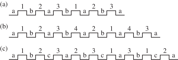
We study the model (1) by the CT-QMC, which evaluates a perturbation expansion stochastically. In the present case, we adopt the hybridization expansion[15]. Since the non-perturbative part is diagonal with respect to $\alpha$ and $\mu$, the efficient algorithm using a ‘segment’ picture is applicable by a slight modification. Figure 1 shows a diagram of a configuration of order $V^{6}$. Spin states $\mu_{i}$ and channel states $\alpha_{i}$ appear alternately, which are hereafter referred to as segment and anti-segment, respectively. In general, a configuration of order $V^{2k}$ is represented by $q_{k}\equiv\{\tau_{i},\tau_{i}^{\prime},\alpha_{i},\mu_{i}\}$. The trace over the local states is thus taken into account graphically. On the other hand, the trace over conduction electrons is evaluated based on Wick’s theorem. A Monte Carlo sampling is performed in the configuration space composed of $k$ and $q_{k}$.

We perform the following update processes: (i) addition/removal of a segment or an anti-segment, and (ii) exchange of spin or channel indices. Fig. 2(a) shows the addition of a segment. The index $\mu$ of the segment is randomly chosen, and accordingly the update probability differs from that in ref. \citenWerner06 by a factor of $N$. When either $N$ or $M$ is larger than 2, the ergodicity is not satisfied only by process (i). For example, configurations shown in Fig. 3 cannot be reached. This problem can be solved by introducing a process shown in Fig. 2(b), which exchanges the spin indices. We perform a similar update to exchange the channel indices as well.

In the simulation, we observe negative weight configurations for $N=M>2$. However, since their contribution is less than 10% in the parameter range shown in this paper, the sign problem has little effect on the simulation.

In this paper, we restrict ourselves to $N=M$. We use a rectangular density of states $\rho(\epsilon)=(1/2D)\theta(D-|\epsilon|)$ for conduction electrons with $D=1$. We fix $NV^{2}=0.12$ so that the exponent of the Kondo temperature is the same for different $N$. The width of the localized state $\Delta=\pi V^{2}\rho(0)$ is $\Delta\simeq 0.094$ at most (for $N=2$), and therefore the effect of finite band width may be neglected.

We have presented the impurity Green’s function $G_{f}({\rm i}\epsilon_{n})$ and the self-energy $\tilde{\Sigma}_{f}({\rm i}\epsilon_{n})$ in the non-Fermi liquid state using the CT-QMC extended to the multichannel Anderson model. For $N=M$, $G_{f}$ and $\tilde{\Sigma}_{f}$ are non-analytic at $\omega=0$ as $|\omega|^{1/2}$. The zero-frequency spectrum ${\rm Im}G_{f}(+{\rm i}0)$ does not depend on the excitation energy $E_{\rm ex}$, and correspondingly ${\rm Im}\tilde{\Sigma}_{f}(+{\rm i}0)$ has a finite value. These values depend only on $N$ ($=M$), and seem to be expressed as eqs. (3), (7) and (8). An analysis of general $N$, $M$ is left for future work.

We acknowledge Prof. Y. Kuramoto for comments on the manuscript. This work was supported by a Grant-in-Aid for Scientific Research on Innovative Areas “Heavy Electrons” (No. 20102008) of the Ministry of Education, Culture, Sports, Science, and Technology, Japan.

References

- [1] P. Nozières and A. Blandin: J. Phys. (Paris) 41 (1980) 193.
- [2] D. L. Cox and A. Zawadowski: Adv. Phys. 47 (1998) 599.
- [3] D. L. Cox and A. E. Ruckenstein: Phys. Rev. Lett. 71 (1993) 1613.
- [4] A. W. W. Ludwig and I. Affleck: Phys. Rev. Lett. 67 (1991) 3160; I. Affleck and A. W. W. Ludwig: Phys. Rev. B 48 (1993) 7297.
- [5] A. Jerez, N. Andrei, and G. Zaránd: Phys. Rev. B 58 (1998) 3814.
- [6] K. Yamada: Electron Correlation in Metals (Cambridge University Press, Cambridge, U.K., 2004).
- [7] K. Yosida: Theory of Magnetism (Springer-Verlag, Berlin, 1996).
- [8] A. Schiller, F. B. Anders, and D. L. Cox: Phys. Rev. Lett. 81 (1998) 3235.
- [9] C. J. Bolech and N. Andrei: Phys. Rev. B 71 (2005) 205104.
- [10] F. B. Anders: Phys. Rev. B 71 (2005) 121101.
- [11] H. Johannesson, C. J. Bolech and N. Andrei: Phys. Rev. B 71 (2005) 195107.
- [12] J. Kroha, P. Wölfle, and T. A. Costi: Phys. Rev. Lett. 79 (1997) 261; J. Kroha and P. Wölfle: Acta Phys. Pol. B 29 (1998) 3781.
- [13] A. Tsuruta, Y. Ōno, T. Matsuura, and Y. Kuroda: J. Phys. Soc. Jpn. 66 (1997) 3528.
- [14] A.N. Rubtsov, V.V. Savkin and A.I. Lichtenstein: Phys. Rev. B 72 (2005) 035122.
- [15] P. Werner, A. Comanac, L.de’ Medici, M. Troyer and A.J. Millis: Phys. Rev. Lett. 97 (2006) 076405; P. Werner and A.J. Millis: Phys. Rev. B 74 (2006) 155107.
- [16] J. Otsuki, H. Kusunose, P. Werner and Y. Kuramoto: J. Phys. Soc. Jpn. 76 (2007) 114707.