Numerical Study of the Two Color Attoworld
Abstract:
We consider QCD at very low temperatures and non-zero quark chemical potential from lattice Monte Carlo simulations of the two-color theory in a very small spatial volume (the attoscale). In this regime the quark number rises in discrete levels in qualitative agreement with what is found analytically at one loop on with [1]. The detailed level degeneracy, however, cannot be accounted for using weak coupling arguments. At each rise in the quark number there is a corresponding spike in the Polyakov line, also in agreement with the perturbative results. In addition the quark number susceptibility shows a similar behaviour to the Polyakov line and appears to be a good indicator of a confinement-deconfinement type of transition.
Keywords:
QCD at non-zero chemical potential; lattice gauge theory1 Introduction
The study of QCD at low temperature and non-zero chemical potential is complicated by the presence of the sign problem: setting results in a complex action which prevents the importance sampling necessary for conventional methods of lattice simulation. Perturbation theory is also not valid in this regime in the infinite volume limit because the coupling strength is large. One method of avoiding the sign problem is to study a theory which may closely resemble QCD, specifically the two-color theory, for which the action is real even for non-zero chemical potential. This is the theory we study in this paper. Another technique which works in the low temperature and non-zero chemical potential regime is to compactify the spatial volume onto a manifold with size ; this is the limit of the attoworld and here it is possible to calculate using perturbation theory.
In [1] we calculated the phase diagram of QCD in the - plane on , where is the radius of , considering both , and also for which there is a thermodynamic limit and genuine phase transitions can occur. In a small volume, quarks occupy well-defined single-particle states of finite degeneracy, whose energies are well-separated on the scale defined by (given by the inverse radius of the ). In the large theory, we found that for there is a rich structure of third-order Gross-Witten-like transitions between “confined” and “deconfined” phases (the names refer to the behaviour of the Polyakov line) as the chemical potential passes one of the quark energy levels. The interpretation is that as scans past a level, the quarks fill the level and the system becomes de-confined in the sense that the Polyakov line gains a non-vanishing expectation value. As increases further, the system re-enters the confined phase where the Polyakov line vanishes. The Polyakov line consequently exhibits a peak with discontinuous slope where the phase transitions occur. At finite , similar peaks are seen, but in this case the curve is smooth since there are no phase transitions away from the thermodynamic limit.
The analysis of [1] was done in the one-loop approximation and it is important to consider non-perturbative effects. In this paper we calculate several observables using lattice gauge theory simulations of QCD with (also known as Two Color QCD or QC2D) formulated on small tori, and at very low temperatures, using lattices. We will find that the quark number, Polyakov line, and quark number susceptibility qualitatively resemble the results from perturbation theory on [1] but with noticeable quantitative differences, which may result from working at larger coupling strength, or may be due to the formulation of the theory on a different manifold, an effect which may be possible in the small volume limit in which we work. We supplement further the perturbative results of [1] with numerical calculations of the relevant observables on for . In neither case is there a thermodynamic limit, as both and () are finite. These findings reinforce our observation, made in [1], that deconfining behaviour in gauge theories with appears to be associated with a non-zero density of gapless quark states.
In the next section we introduce the lattice formulation of QCD with gauge group SU(2), and in Section 3 briefly outline the behaviour of the lattice model on a finite system as is increased in the non-interacting limit. An important difference with the perturbative approach of [1] is that as well as an IR cutoff , there is in this case an explicit UV scale associated with the lattice spacing . Section 4 presents results from non-perturbative lattice simulations of the interacting theory, where possible comparing them with the equivalent quantities calculated on with and . We conclude with a brief discussion.
2 Formulation and Simulation of the Lattice Model
We begin by defining the action for Two Color QCD on a hypercubic lattice [2], choosing units where the lattice spacing , and a Euclidean spacetime index :
| (1) |
where , is the oriented product of 4 SU(2)-valued link fields around the sides of an elementary plaquette in the - plane, , are Grassmann-valued quark fields located on the lattice sites, whose index runs over flavors, and is the quark chemical potential. The quark matrix utilises the Wilson formulation for lattice fermions:
| (2) |
The parameter , where is the bare Yang-Mills coupling, and the hopping parameter is related to the bare quark mass via
| (3) |
In the free field limit , but since the action defined via (2) has no manifest chiral symmetry, its value is subject to quantum corrections and must in general be determined by simulation; chiral symmetry is then only recovered in the limit . Chemical potential is introduced via the orthodox prescription of treating as a constant imaginary timelike abelian gauge potential [3].
For the system in hand it is possible to calculate quantum corrections non-perturbatively using numerical Monte Carlo simulation [2, 4]. The simulation proceeds via an orthodox hybrid Monte Carlo (HMC) algorithm, which unlike the case of QCD is not subject to the notorious Sign Problem for , since the functional measure remains real and therefore positive due to the special SU(2) property
| (4) |
where the Pauli matrix acts on color indices. The most important thermodynamic observable in the presence of chemical potential is the quark density
| (5) |
The other key observable in this study is the Polyakov line, defined in terms of link variables by
| (6) |
3 Free field limit results ()
In the free field limit the quark density (5) on a finite lattice can be evaluated via a simple mode sum [2]. The results for a system are shown as a function of for various in Fig. 1.

The numbers are expressed in the form , where is the maximum quark density which can be accommodated on the lattice as a result of the Pauli principle, essentially one quark of each spin, flavor and color per site. The existence of such a “saturated” system is a consequence of having an explicit ultra-violet cutoff; there is no corresponding feature in the results of [1] which were obtained in the continuum.
Fig. 1 shows increasing monotonically with , but with a step-wise behaviour rather than the expected in the thermodynamic zero-temperature limit. A physical way of understanding this is that for a system with , the thermal smearing of the Fermi surface associated with degenerate quarks will be much smaller than the spacing between plane wave modes, meaning that the Fermi surface will be markedly non-spherical [5]. Indeed, close inspection of the figure reveals that the total quark occupancy on the plateaux have respectively , 7, 19 and 27, implying the existence of well-separated energy levels (on the scale of ) with degeneracies 1, 6, 12 and 8. These are readily identified with the plane-wave states available on a system, which in units of the mode spacing take the form , , and respectively. The figure also shows that varying has a small effect on the energies of these discrete levels, given by the value of at the riser of each step, but none on their degeneracy. For the value corresponding to free massless quarks, the onset at which rises from zero takes place at ; this threshold shifts to larger for .
The results for are thus in qualitative accord with the one-loop findings of [1], except in that case the equivalent degeneracy of the th level is given by , with as appropriate for angular momentum eigenstates on a hypersphere. Another difference is that for massless quarks the hypersphere levels are equally spaced. It is thus reasonable to anticipate that the structure of Fig. 1 would remain stable under weakly coupled quantum corrections, i.e. with large but finite.
4 Results for the Interacting Case
In this section, we first present numerical results obtained with at two coupling strengths and , close to the weak-coupling limit. This will enable an estimate of how quantum corrections evolve with coupling, but it should be noted that both values are considerably weaker than those employed in the studies [2, 4] which explored significantly larger volumes. The lattice spacing at was determined via the string tension to be fm, implying that corresponds to a system size considerably smaller than a fermi even at these stronger couplings. Using the one-loop beta-function estimate with , we can be confident that the simulations described here definitely probe the attoworld. Another important difference is that in previous work a diquark source of the form (in effect a Majorana mass for the quarks) was introduced; this had the effect of mitigating infra-red fluctuations associated with the Goldstone modes induced by superfluidity due to diquark condensation, thus improving the performance of the HMC algorithm. In the current work we judged this would not be needed for such small systems; even so it was found that, eg. the number of conjugate gradient iterations required for the HMC acceptance step occasionally exceeded (see Fig 10 below).

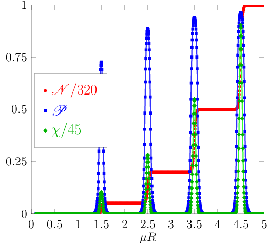
Fig. 2 shows the results of a scan along the -axis for . For each value of 2000 HMC trajectories of mean length 0.5 were accumulated. The quark density is calculated according to eq. (5), and we define the quark number susceptibility by its derivative with respect to ,
| (7) |
In principle in lattice QCD is calculated in terms of correlations of quark bilinears [6], but in this study since we have a finely-spaced comb of -values we adopt the more pragmatic route of approximating the derivative in (7) by a finite difference.
It is interesting to compare the lattice results with those of a one-loop calculation on . Figure 3 shows the same quantities (though normalized differently) on and plotted against , where is the radius of (for comparison in Fig. 2). The action of QCD on to 1-loop order is given as in [1], and was originally derived in [7] for more general matter content. At low temperatures the partition function is given by
| (8) |
where , , and is given by
| (9) |
where is the quark mass. In Figure 3, the Polyakov line , quark number , and quark number susceptibility , are all derived from the partition function. These are given by
| Polyakov line: | (10) | ||||
| Quark number: | (11) | ||||
| Quark number susceptibility: | (12) |
Note that with this normalisation is an extensive quantity. Qualitatively the lattice results of Figure 2 and the perturbative results on in Figure 3 appear similar: the fermion number rises in discrete levels, and there is a spike in the Polyakov line and the quark number susceptibility at each level transition. However, there are noticeable differences in the shape of the curves during the transitions. The differences between the lattice and perturbative results could be due to working at different interaction strengths. Also, in small volumes effects from considering different manifolds should be more apparent. In what follows we discuss each of the observables calculated at on the lattice in detail, comparing with the results from where appropriate.

Before discussing each observable in detail it is interesting to see what happens when we increase the interaction strength a little more. Fig. 4 shows the same scan of the -axis at stronger gauge coupling . The level degeneracies corresponding to the occupancies on the staircase are identical to those at indicating that the system responds adiabatically in this coupling range. Moreover, the shell energies given by the risers are also little changed, showing that dependence of the levels on is weak. The behaviour of also suggests a similar relation with , albeit with a much reduced signal which can be attributed to much larger quantum fluctuations at this stronger coupling.
The most striking feature of Figs. 2,4 is the qualitative similarity of the relation between and to that found using weak coupling methods on the hyperspherical attoworld of Figure 3 and of the results in [1]. The numerical results reinforce the claim that deconfining behaviour is correlated with a partially filled energy level or “shell” in the box, implying that deconfinement is associated with a non-zero density of gapless states.
4.1 Quark number density
The weak-coupling results for in Figure 2 exhibit a staircase structure similar to that of Fig. 1, but with two important differences. Firstly, the onset value of is considerably larger, and secondly the degeneracies of the discrete levels are now 8, 8, 6, 16, 8 and 8, with the understanding that each of these numbers should be multiplied by a factor (see next paragraph). It should also be noted that over certain -ranges is double-valued; this arose from simulations where two distinct and apparently stable, or at least metastable, states of the system were found (in such cases the state with larger is shown with open symbols). In some cases “tunnelling” events from one state to the other occurred as the simulation proceeded. Since both and are small, and we are accordingly far from any thermodynamic limit, there seems to be no obvious criterion for deciding which if either is the “true” ground state.
Before commenting further on the level degeneracies, we wish to highlight an important constraint on the interacting theory. The grand canonical partition function can be written
| (13) |
where is the canonical partition function evaluated in the sector with fixed particle number . On one of the steps in Fig. 2 where is approximately constant, it must be the case that , implying that the sum in (13) is saturated by one particular value of , and hence that . Now, using the Fourier representation of the -function, (13) may be inverted to yield
| (14) |
i.e. the canonical partition function is the th Fourier component of the grand canonical partition function evaluated with imaginary chemical potential . However, it is known [8] that the centre symmetry of the pure gauge theory can be extended to the case of matter with imaginary chemical potential, resulting in a periodicity
| (15) |
Eqns. (13,15) together imply is only non-vanishing for integer, or in other words that the canonical partition function is only defined for sectors of zero -ality. Notice that, while the weak coupling analysis is obviously consistent with this constraint, the values of observed on the steps of Fig. 2 are, indeed, multiples of which is a far from trivial check on the lattice analysis.
In fact, the observed pattern of degeneracies 8, 8, 6, 16, 8, 8 appears impossible to explain in terms of single-particle plane wave states, in important contrast to the free case Fig. 1. We conclude that while the staircase behaviour of appears to be a universal feature of attosystems, non-perturbative effects continue to play an important role in determining the spectrum.

On the quark number at low temperature and zero quark mass is given by [1]
| (16) |
Here the level structure arises because of the contribution from the Fermi-Dirac distribution function
| (17) |
which, at low temperatures, is when is larger than an energy level , and zero otherwise. Thus the number of quarks at each level is a sum over the fermion degeneracies of all levels with :
| (18) |
A plot of the quark number on as a function of for , and , is given in Figure 5. In both cases the quark number is symmetric about the mid-point of the transition at , in that the level transition starts and finishes at the same rate, in contrast to the lattice results of Fig. 2. The results also shown (from [1]), exhibit quite clearly the two Gross-Witten-type phase transitions as the points of non-analyticity where the quark number first turns on and then saturates as is increased.
4.2 Polyakov line
In addition to quark density , the other important observable monitored was the Polyakov line defined in Eqn. (6). In theories without fundamental matter is an order parameter for deconfinement; even in the presence of quarks it can be related to the free energy of a static fundamental source via , and lattice studies of eg. the thermal transition in QCD observe a sharp increase in around the deconfining temperature. The behaviour of in systems with and is considerably less studied, although intriguing results have been reported in [2, 4]. Note that for there is no distinction between and defined using the inverse link variables in (6).
Fig. 2 shows that the Polyakov line exhibits a complicated behaviour: in regions where is constant its value is small, possibly consistent with zero, but in regions where is changing , implying deconfinement. In fact it exhibits rather sharp maxima over at least six distinct ranges of : its numerical value is in accord with expectations that the theoretical maximum value of 1 is renormalised downwards due to quantum fluctuations [9]. When increases to one of its plateaux over a very short -interval, the transition from to is very sudden; on other occasions when the behaviour between plateaux is an extended S-shape, has a more symmetrical peak. This seems to be true even in regions where both confining and deconfining states are found.

Fig. 6 focusses on the range over which the second shell is gradually occupied and rises from zero to its maximum value. The histogram shows that the fluctuations throughout, but that the distribution evolves from being symmetrically centred on zero at to being highly skewed at .


The Polyakov lines on as a function of are shown in Fig. 7 (left) for and . For , and the Polyakov line is symmetrical around each energy level . It is important to note that this is not the case for , where and these are individually asymmetrical around each energy level, though mirror images of each other. This reflects that fact that in general fundamental and antifundamental test charges respond differently to a background density of fundamental charge. As remarked above, the lattice results show both features which are approximately symmetrical as well as some which are clearly skewed, in apparent contradiction with the prediction shown in Fig. 7.
4.3 Quark number susceptibility
To a very good approximation Fig. 2 shows that ; indeed, the quark number susceptibility is often taken as an alternative signal of deconfinement in lattice studies of the thermal QCD transition [10].
Figure 7 (right) shows the quark number susceptibility from perturbation theory on for and . For the quark number susceptibility is calculated by numerical integration:
| (19) | ||||
where
| (20) |
and
| (21) |
To obtain the result the quark number susceptibility is calculated by taking the derivative of the result for the quark number in [1]. It is only non-zero while a level transition is taking place; near the step the expression is
| (22) |
where is determined as in [1] from numerical inversion of
| (23) |
and is given by (18). It is clear from eq. (22) and Figure 7 (right) that for another derivative of with respect to will result in discontinuities at the beginning and end of each level transition, indicating that these correspond to third order transitions as predicted in [1].
We note that the level structure of the particle number and corresponding susceptibility spikes were also observed in simulations of the non-linear sigma model [11].
4.4 Quark–antiquark condensate

Next we discuss another fermionic observable, the quark–antiquark condensate, which requires a non-perturbative calculation. For Wilson lattice fermions (2):
| (24) |
Because (2) has no chiral symmetry, this bilinear has no interpretation as an order parameter, but does yield information on the conformal anomaly [2]. The data, however, echo the structure of Fig. 2: is approximately constant in -ranges where there are only filled shells, and changes rapidly in the same regions where changes rapidly, corresponding to a partially-filled shell.
4.5 Gluonic observables


It is also of interest to consider gluonic observables. The simplest local gauge-invariant gluon observable is the plaquette . In a non-Lorentz invariant system such as one with it is helpful to define
| (26) |
The normalisations ensure in the limit. We then consider in Fig. 9 both the average plaquette and the difference , which is proportional to the gluon energy density
| (27) |
where is a renormalisation factor calculable in perturbation theory [12].
The average plaquette has a value extremely close to unity, as befits such a weak coupling. It has a non-monotonic variation with , qualitatively similar to the behaviour found on larger systems in [2, 4]. The decrease at large is readily understood as a consequence of saturation : in this regime screening due to virtual quark – antiquark pairs is suppressed due to Pauli blocking, and hence many gluonic observables revert to their values in the quenched theory, which has in effect a larger lattice spacing and hence a larger departure from the free-field value. At , where the average plaquette dips below its value at , the ratio , to be contrasted with the corresponding value observed at [4].
The difference also shows non-monotonic behaviour; its negative value makes it hard to interpret as a physical energy density, and probably arises as an artifact of the lattice aspect ratio . Both plots hint at a finer structure, such as a dip at . Curiously this does not appear to match any interesting region of Fig. 2, except in the sense that both confining and non-confining solutions appear to be stable here.
4.6 Conjugate gradient iterations

Finally, Fig. 10 plots the number of iterations of the conjugate gradient algorithm required to invert to some pre-specified accuracy (in this case such that the average norm of the residual vector should not exceed per site, spin and color) as a function of . This quantity carries physical information since it is roughly inversely proportional to , where is the complex eigenvalue of closest to the origin. Fig. 10 suggests that the smallest eigenvalue evolves smoothly so long as is smooth, but jumps sharply at the same points where is discontinuous. Note that the eigenvalue is always smallest in deconfined regions where , again consistent with the picture of a non-zero density of gapless modes. Interestingly, this pattern is also respected by the alternative solutions corresponding to the open symbols of Fig. 2, suggesting that at these points the simulation sometimes evolves smoothly with , and at other times jumps to a new ground state with significantly smaller ; further studies on systems with varying (correpsonding to varying ) might clarify the situation here.
5 Summary
This paper has followed up the study of QCD at non-zero chemical potential on spaces defined by a scale initiated in Ref. [1] by presenting Monte Carlo results for the case which is simulable using orthodox lattice gauge theory techniques. We have shown that the two principal qualitative features of the perturbative calculation on the hypersphere, namely that the quark density is a step-wise function of , and that the Polyakov line is significantly different from zero only in the -ranges where is rising, persist on the three-torus even once non-perturbative effects are correctly included. The staircase form of is indicative of a series of widely separated sets of physical states akin to the shell structure of, say, a nucleus. Moreover we have identified a further relation, , which seems to be respected equally well in both approaches. These results lend support to the interpretation of as an alternative indicator of confinement/deconfinement in systems with fundamental matter, and hint at a relation between deconfinement and a non-vanishing density of gapless states (in other words, the existence of a “conduction band”).
However, the two approaches differ in their detailed predictions for the shell degeneracies. Comparison of simulation results at two different values suggests the system evolves adiabatically with coupling, but it has not proved possible to interpret the levels in terms of the single-quark states underpinning the perturbative approach, and a full explanation of the structure revealed in Fig. 2 is still missing.
In addition, identification of the correct ground state of the system as is varied was troublesome due to the apparent existence of more than one “solution” stable under HMC evolution (in fact, this proved to be a much more serious problem in pilot studies on , and persuaded us to switch to a system where was not a multiple of ). In conventional simulation campaigns such ambiguities are normally resolved by taking the thermodynamic limit, but here and are both finite. It would, of course, be interesting to try a simultaneous tuning of and , keeping fixed, but this requires resources considerably beyond what we have been able to expend. In any case, more general questions about how both thermodynamic and zero temperature limits are approached would also be interesting to explore.
6 Acknowledgements
This project was enabled with the assistance of IBM Deep Computing.
References
- [1] S. Hands, T.J. Hollowood and J.C. Myers, JHEP 1007 (2010) 086 [arXiv:1003.5813 [hep-th]].
- [2] S. Hands, S. Kim and J.I. Skullerud, Eur. Phys. J. C 48 (2006) 193 [arXiv:hep-lat/0604004].
- [3]
P. Hasenfratz and F. Karsch,
Phys. Lett. B 125 (1983) 308;
J.B. Kogut, H. Matsuoka, M. Stone, H.W. Wyld, S.H. Shenker, J. Shigemitsu and D.K. Sinclair, Nucl. Phys. B 225 (1983) 93. - [4] S. Hands, S. Kim and J.I. Skullerud, Phys. Rev. D 81 091502(R) (2010) [arXiv:1001.1682 [hep-lat]].
- [5] S. Hands and D.N. Walters, Phys. Lett. B 548 (2002) 196 [arXiv:hep-lat/0209140].
- [6] S.A. Gottlieb, W. Liu, D. Toussaint, R.L. Renken and R.L. Sugar, Phys. Rev. Lett. 59 (1987) 2247.
- [7]
B. Sundborg,
Nucl. Phys. B 573 (2000) 349
[arXiv:hep-th/9908001];
O. Aharony, J. Marsano, S. Minwalla, K. Papadodimas and M. Van Raamsdonk, Adv. Theor. Math. Phys. 8 (2004) 603 [arXiv:hep-th/0310285]. - [8] A. Roberge and N. Weiss, Nucl. Phys. B 275 (1986) 734.
- [9] S. Gupta, K. Huebner and O. Kaczmarek, Phys. Rev. D 77 (2008) 034503 [arXiv:0711.2251 [hep-lat]].
- [10] A. Bazavov et al., Phys. Rev. D 80 (2009) 014504 [arXiv:0903.4379 [hep-lat]].
- [11] D. Banerjee and S. Chandrasekharan, Phys. Rev. D 81 (2010) 125007 [arXiv:1001.3648 [hep-lat]].
- [12] F. Karsch, Nucl. Phys. B 205 (1982) 285.