Numerical solution of the nonlinear evolution equation at small with impact parameter and beyond the LL approximation
Abstract
Nonlinear evolution equation at small with impact parameter dependence is analyzed numerically. Saturation scales and the radius of expansion in impact parameter are extracted as functions of rapidity. Running coupling is included in this evolution, and it is found that the solution is sensitive to the infrared regularization. Kinematical effects beyond leading logarithmic approximation are taken partially into account by modifying the kernel which includes the rapidity dependent cuts. While the local nonlinear evolution is not very sensitive to these effects, the kinematical constraints cannot be neglected in the evolution with impact parameter.
Keywords:
quantum chromodynamicsI Introduction
High energy limit in Quantum Chromodynamics is one of the most intriguing problems in strong interaction physics. Since the Large Hadron Collider has recently opened a new kinematic regime, it is of vital importance to understand how one can calculate the cross section at high energies from basic principles in QCD. The BFKL equation obtained in the Regge limit of QCD [1, 2, 3, 4] predicted fast growth of the cross section with the energy, due to the exchange of the hard Pomeron. This behavior is however known to violate the unitarity bound of the scattering amplitude. Higher order corrections to the BFKL [5, 6, 7, 8, 9, 10, 11, 12, 13] tame the growth but other terms due to the parton recombination [14] and multiple Pomeron exchanges have to be taken into account in order to guarantee the unitarity of the scattering amplitudes.
The Balitsky-Kovchegov equation was derived in [15, 16] in the dipole approach [17] to high energy scattering in QCD and independently in the formalism for the operator product expansion at high energy as an evolution of the Wilson line correlators with respect to the rapidity [18, 19, 20, 21, 22]. This equation also emerges in the Color Glass Condensate formalism as a limit of the JIMWLK functional equation [23, 24, 25, 26, 27], see also [28, 29]. The BK equation was shown to be equivalent to the BFKL evolution with the triple Pomeron vertex [30, 31] when the latter one is restricted to the Möbius space of functions [32].
Numerous analyses of BK equation which were performed up to date, see for example [33, 34, 35, 36, 37], focused on finding the solutions to this equation under the assumption that the amplitude does not depend on the impact parameter but only on a dipole size and rapidity. This assumption makes the equation relatively easy to solve (at least numerically). Usually one is justifying this approximation by considering the scattering off a very large target, therefore bringing a large scale into the problem. This results in breaking the symmetry between the infrared and ultraviolet regions even in the case of the fixed coupling by generating a saturation scale which acts as a boundary and suppresses the diffusion into the infrared region [35, 38]. In the momentum space this approximation is equivalent to taking the forward limit in the evolution with the simplifying approximation on the triple Pomeron vertex resulting in zero momentum transfer through the vertex in both reggeized gluon pairs [39]. On the other hand, the kernel of the equation has the property that it is invariant with respect to the translations, dilatations, rotations and inversions, which are Möbius transformations. Therefore the solutions to the nonlinear equation should also reflect this symmetry properties, at least in the leading-logarithmic, fixed coupling limit. On a deeper level it is related to the Möbius invariance of the reggeized gluon transition vertex which was demonstrated explicitly [40]. In the relation to the experiment, the detailed knowledge about the dynamics and expansion in impact parameter is of the utmost importance for the qualitative and quantitative description of the multiparticle production in hadronic collisions.
In this paper we analyze this equation numerically including the full impact parameter dependence. This is an extension of the previous work [41] where this type of analysis was performed, see also [42]. We significantly improve over [41] the numerical accuracy and technique which enables us to evolve the equation much faster and to very high values of rapidity, of the order of . In this way one can more accurately extract the asymptotic values of different exponents which govern the growth of the saturation scales in this equation. We confirm the results of [41], on the dependence of the scattering amplitude as a function of dipole size and demonstrate that it vanishes for large dipole sizes. We also find the fast diffusion of the solution in impact parameter space and recover the power tails. The saturation scale both for small and large dipoles is extracted, and the dependencies on the impact parameter and rapidity are found. The results of the solutions to the equation in the leading logarithmic approximation (LL) are compared with the modified version of the equation proposed in [43]. The modified version contains the cutoffs in rapidity which originate from kinematical constraints. These cutoffs contain kinematical constraints in only approximate way but we know from the analysis of forward BFKL in momentum space that these constraints are known to reduce the speed of the evolution in a significant way [44], (for a related analysis on impact parameter dependence in nonlinear equation and the energy conservation see [45]. The BK without impact parameter dependence and with rapidity cutoffs was also analyzed in [35, 46]). We also include running coupling in our analysis and find that the effect of the running coupling is quite different than in the case without the impact parameter. In this paper we consider a prescription for the running coupling with the external dipole as the scale as well as the prescription derived in [47]. The impact parameter dependent equation is extremely sensitive to the large dipole sizes and this is the region where the running coupling is very large and needs to be regularized by some other mechanism.
In this analysis we did not attempt to regularize the large dipole size region in any way. It is at present totally unclear how confinement effects should be consistently included in the dipole formalism. Of course, for any phenomenological applications such cut should be included, perhaps similarly to what was done in [48]. As we were interested in general properties of the evolution we did not attempt here to introduce additional cuts on large dipole sizes (via masses), which would interfere with the specific dynamics of the evolution.
The paper is organized in the following way. In the next section, Sec. II we briefly present the BK equation and discuss the modified version which includes the cutoffs in rapidity. In Sec. III we describe the numerical methods of finding the solution. In Sec. IV we first show the results of the solution without the impact parameter and extract the saturation scale for both the LL and the modified equation. In Sec. V we present the solutions with impact parameter. We discuss the form of the amplitude as a function of the dipole size, extract the saturation scales (both for small and large dipoles), and discuss the form of the impact parameter profile which emerges in the evolution. We present the solutions both in the case of the LL and for the modified kernel. Using the representation in terms of the conformal eigenfunctions we discuss the origins of different peaks in the amplitude as well as present estimates for the rapidity dependence of the small and large dipole saturation scales and the expansion radius in impact parameter. We also present the estimate of the cross section of the black disc radius and its dependence on the rapidity. In Sec. VI we discuss the results with the running coupling, both for the case without and with impact parameter dependence, and for two different prescriptions of the running coupling. Finally, in Sec. VII we state our conclusions.
II BK Kernel in LO and beyond
In the leading logarithmic approximation in , the nonlinear Balitsky-Kovchegov [15, 16, 18, 19, 20, 21, 22] evolution equation derived in dipole picture [17] has the following form
| (1) |
where is the strong coupling constant. Here, is the dipole-nucleus scattering amplitude, and are two-dimensional vectors of the transverse position of the dipole ends. Alternatively, one can introduce the vector denoting the dipole size , and the impact parameter . Thus in general, the amplitude depends on the four degrees of freedom in transverse space and rapidity, , playing the role of the evolution parameter. The transverse part of the LL kernel
is conformally (Möbius) invariant in 2-dimensions. Here, we introduced a more compact notation denoting , and is the longitudinal momentum fraction so that rapidity is .
To obtain the solution of this equation, one has to specify an initial condition at : .
The amplitude in (1) is given by the following correlator
| (2) |
where the trace is done in the color space, and the eikonal factor is defined as the path ordered exponential with the gauge fields (in the gauge )
| (3) |
The averaging in (2) is performed over an ensemble of classical gauge fields.
The next-to-leading logarithmic corrections to the BK equation have been computed in [47, 49]. It would be instructive to perform the analysis of the BK equation with full NLL approximation. Due to the complicated form of this kernel we are not trying to solve it here. What we consider instead, is the equation with two important modifications. The first one is the running coupling correction, which we analyze in Sec. VI of this paper. The second one is the subleading correction coming from the kinematical corrections, included in the form of the modified kernel proposed in [43].
The soft gluon approximation performed in [17] was crucial in order to factorize the the branching kernel for the gluon emissions. In [43] a modified version of the kernel was proposed, which includes part of the subleading corrections coming from the kinematics. By taking into account an improvement in kernel in which the value of energy denominator is obtained from the invariant mass of the produced gluon pair. This leads to a new color dipole kernel which has the form
| (4) |
where is the modified Bessel function. The modified kernel becomes equivalent to the leading logarithmic kernel for and but differs significantly otherwise. To be precise, the production of larger dipole sizes is exponentially suppressed above the cutoff size which depends on the longitudinal momentum fraction of the soft gluon. The modified kernel introduces corrections at all orders beyond the leading logarithmic approximation. The suppression of the large dipole emission implies also a suppression of the diffusion in the impact parameter. An alert reader might notice that the above modified kernel is not conformally invariant. This is due to the fact that in [43] only part of the kinematical corrections were taken into account resulting in kernel (4). In general there should be also a cutoff on small dipoles, similarly to what was done in [50], which would yield conformally invariant kernel. We postpone the derivation and numerical analysis of such kernel to a later work.
In what follows we will analyze both forms of the equations numerically, taking into account also running coupling corrections. We shall demonstrate that the sensitivity to the subleading corrections strongly depends on the type of approximation one is working on, i.e. whether the solutions are impact parameter dependent or not.
III Numerical Methods
The BK equation was solved numerically by discretizing the scattering amplitude in terms of variables , where is the angle between impact parameter and dipole size . There is an additional angle, which reflects the overall orientation, we assumed that the solution is rotationally invariant. The amplitude was placed on a grid with dimensions . It was found that the number of points in the grid was less important than the absolute limits on the grid and the number of integration regions. The limits of the grid were in and . We note that, the grid limits of and cannot not be set independently due to the correlations in dipole size and impact parameter. The initial condition at rapidity was chosen as in Ref. [41] to be of the Glauber-Mueller [51, 52] form
| (5) |
This is the form of the scattering amplitude at the initial rapidity. We note that in this analysis the constants are arbitrary and have not been fit to any experimental data. The initial condition (5) has the property that it reaches unity when the dipole size is large and it goes to zero for large values of impact parameter by the steeply falling profile in . The amplitude is evolved in small steps as it was found that the smaller spacings had no significant effect on the accuracy of the evolution of the amplitude. Below, we denote integration over simply by and this is understood to absorb the kernel as well as a measure for ease of notation in this section. The basis of the method for the solution is the same as utilized in Ref. [41] and we briefly outline it below. After one step of evolution from to the equation (1) becomes
| (6) |
The lowest approximation for this equation is
| (7) |
The superscript 1 denotes the first approximation while the superscript 0 denotes the initial condition. The accuracy of the equation is measured by the relative difference of the approximation defined by . If this is less than some required accuracy then the value of is taken as the scattering amplitude at . In our case the relative accuracy was set to be equal . If the accuracy condition is not satisfied, then we can find a second approximation by utilizing linear interpolation . By using this linear interpolation in the right hand side of 6 the expression for the next iteration can be attained
| (8) | |||||
If the accuracy condition mentioned earlier is still not satisfied this can be repeated by utilizing . The number of iterations required to reach this level of accuracy varies on how close one is to the initial condition, and the exact form of the equation (kernel used, running coupling form, etc). Near the initial conditions it could take upwards of ten iterations but far away from the initial condition two or three iterations are usually sufficient to obtain the accuracy assumed. With this in mind an algorithm was written so that the iteration number was not fixed but only continued until the desired accuracy was reached. Once the amplitude has been found for that takes the place of in the numerics and the procedure is repeated to find the amplitude at . In this way the amplitude is evolved numerically to higher rapidities.
As was mentioned earlier the number of points in the grid was not as important as the number of integration regions the program executes to get a good solution. For our limits it was found, that breaking the range into at least 20 integrations was needed. This meant there would be an incredible number of function evaluations and in order to reach any useful rapidity on a standard dualcore machine would take upwards of a month. The program was parallelized using the MPI (Message Passing Interface) library so it could be used with computer clusters to run the program. Each run took approximately three days to run on 32 linked processors and generated a total of 5 gigabytes of data.
IV Results without impact parameter dependence
In this section we briefly present the results of the numerical solution without impact parameter dependence. This was of course done in many previous works [33, 34, 35, 53], but we repeat this analysis below for several reasons. First of all, we wanted to have benchmark for the comparison of the solutions. Secondly, we wanted to perform the analysis of the modified BK equation with Bessel function kernel, a computation not performed earlier in the literature.
The BK equation can be evaluated without impact parameter or angular dependence and this greatly reduces the time needed to evolve the scattering amplitude. The initial condition used in this case is taken to be
| (9) |
without an impact parameter profile. This form goes to unity as the dipole size gets large and has a narrow transition region from 0 to 1. The absolute limits on the dipole size here are and the number of points in the grid is 5000. These results are for fixed coupling , the case with running coupling is considered in section Sec. VI.
The solid lines shown in left graph in Fig. 1 correspond to a set of scattering amplitudes found from the LO BK equation at constant rapidity. The result has the well known form of a traveling wave with rapidity playing the role of the time in the evolution. As rapidity increases the front moves towards the small values of dipoles.


Right: plot of the logarithm of the saturation scale as a function of rapidity. The solid line represents the evaluation with LO kernel and the dashed line represents the solution with Bessel kernel. The slope of the curve gives and the three regimes of evolution can be seen. Calculation done for the fixed coupling case and without the impact parameter.
Next, we performed the evolution of the modified equation with the Bessel function kernel and the solutions are illustrated by the dashed lines in Fig. 1. The normalization of the amplitude in the dilute regime is much smaller than the LO case. This is to be expected as the functions fall off faster than the power-like LO kernel. The speed of this evolution can be quantified by the evaluation of the saturation scale. The equation to define saturation scale is
| (10) |
where is a constant between 0 and 1. It determines the point at which nonlinearities begin to become important in the evolution equation. In all the analysis in this paper was chosen. Based on results of [54] we expect the saturation scale to have the following form
| (11) |
where is the BFKL kernel eigenvalue, and . This gives and for the LO kernel. The second term in the exponent is a correction of less than 10 percent compared to the first term for the rapidities which we are considering so we take the saturation scale to be parameterized in this paper by
| (12) |
where is extracted from the numerical solution and is a normalization term. The extracted value for the saturation exponent is for both the LO and Bessel function kernels. The exponent was extracted both for and and it was found to be the same. The values of are evaluated in the region of rapidities where the exponent is constant, i.e. nearly asymptotic. We observed that for the lower rapidities, near the initial condition the exponent slowly increases and at very large rapidities the exponent begins to decrease. The latter effect is due to the absolute limits of the dipole size (or the box in which the equation is being solved). This strongly affects the solution, and one of the effects is to slow down the evolution. This effect can be clearly seen in Fig. 1 where the three regimes are distinct. The first regime is where there are a lot of preasymptotic effects and there is strong dependence on the initial condition and the speed of evolution increases (approximately between 0 and 34 units of rapidity), the regime where evolution is a constant (approximately between 34 and 47 units of rapidity) and finally the regime where box size limits growth (rapidity 47+). These values clearly shift with box size and they also change depending on the value of and to a lesser extent which kernel is used.
The extracted value of the exponent of the saturation scale is consistent with the theoretical predictions of [54]. What is however surprising at first, is the fact that the asymptotic value of is nearly the same for the modified version of the equation. This is also evident by investigating right plot in Fig. 1 where the two saturation scales grow with rapidity in almost exactly the same way. This effect can be easily understood by inspecting the form of the modified kernel
| (13) |
Here and . When is small and the arguments of the Bessel functions are small this expression reduces to the LO kernel. At large rapidities where the exponent is evaluated, is small and thus is also small. The difference between the modified kernel and the LO kernel comes from the regime where the dipole sizes are large, that is when
In this large dipole regime (and for large rapidities), the scattering amplitude is close to unity and the right hand side of the BK equation goes to zero so there is no contribution from that regime. This means that the effect of the infrared modification of the kernel of the type (13) is negligible when the nonlinear evolution is considered. The modified kernel (13) was shown to reproduce the double-logarithmic terms in the exact NLL calculation. These type of terms are known to come from the scale choice in the amplitude, [55, 56, 57].
Two comments are in order here. The first observation is that, as we shall see later, the presence of the impact parameter changes the dynamics significantly, and in this case the dependence on the form of the kernel is more pronounced. In particular, in this case we do find the differences in the evolution speed due to the cutoffs in the infrared. The second comment is that, in order to address the question of the scale choices one needs to take into account the corrections beyond the BK equation. BK equation is highly asymmetric with respect to the target and projectile and therefore cannot address the problems of all the scale choices. The corrections would necessarily have to include the Pomeron loops in order to make the evolution symmetric with respect to the target and projectile. Such formulation has been implemented in a Monte Carlo approach [50, 58, 48, 59] with Pomeron loops effectively taken via so-called dipole swing and with cutoffs both in the infrared and ultraviolet regions.
V Results with impact parameter dependence
V.1 Dependence on the dipole size
In this section we discuss the results which include the impact parameter dependence as well as the angular dependence between the dipole sizes and the impact parameter orientation. Let us first investigate the dependence of the scattering amplitude on the dipole size with fixed impact parameter value. Fig. 2 shows that case of the LO simulation with . The scattering amplitude at small dipole sizes evolves in a similar manner as in the case without the impact parameter.
At large dipole sizes the situation is drastically changed with respect to the translationally invariant case. Here, we observe that the amplitude drops down from the initial distribution and forms a second evolution front. This drop is very rapid compared to the expansion evolution of the small dipole size regime or the large dipole size regime at higher rapidities. The evolution of the front at large dipole sizes can be best seen in Fig. 2 where the steps in rapidity are greater. As discussed in [41] there is a clear physical reason for this effect. For a large dipole, its end points are in the region where there is no gauge field. In this situation the gauge field correlator
| (14) |
vanishes because . In this case the dipole is larger than any of the other scales in the problem, including the impact parameter of the collision. In other words this situation corresponds to the setup of very large dipole scattering on a localized target, and in this case the dipole misses the target, resulting in the vanishing scattering amplitude. This effect is not present in the case where impact parameter dependence is neglected simply because this approximate case corresponds to the infinitely large target.


It is interesting to investigate the dipole size dependence of the amplitude at large values of the impact parameter. There the initial condition, sets the amplitude to zero. The evolution quickly changes this value, and a unique feature of the solution develops. Namely, a peak is formed with the center at the dipole size value which is exactly twice the impact parameter value. The peak grows until saturation is reached and the evolution of the fronts proceeds to the infrared and ultraviolet regions. The discussion about the origin of peaks is given in subsection V.4.


We have repeated this analysis for the case of the modified kernel. As can be seen in Fig. 4 the evolution in the small dipole regime is now quite different from the LO kernel. The evolution is significantly slower in this regime for the Bessel function kernel. Interestingly, the evolution in the large dipole region is slowed too but not as much as for small dipoles. This is best illustrated in Fig. 4 where the evolution has been performed to large rapidities. The origins for this behavior are discussed in detail in the section on the saturation scale and evolution speed.


V.2 Impact parameter profile of the scattering amplitude
Dependence of the dipole amplitude on the impact parameter is illustrated in Fig. 5. The leftmost dashed-dotted line is the initial condition Eq. 5 which has a very steep profile in impact parameter. The evolution of the scattering amplitude towards large values of impact parameter follows the diffusion of large dipoles. The speed of this evolution can be extracted numerically and is determined by the expansion of the black disc radius. We will discuss this quantity in detail in the next section.


Evolution in impact parameter shows a marked change in profile from the steeply falling exponential in the initial condition. This is better illustrated in right plot in Fig. 5 where we replot the impact parameter using the logarithmic scale in scattering amplitude. The profile changes from the exponential to a power tail at small scattering amplitudes. This can be seen as an ’ankle’ in the curves of constant rapidity. The origin of this power-like tail was discussed in detail in Ref. [41]. These power tails are also present in the modified kernel. In the latter case however there is a slower evolution of the profile towards the large values of impact parameters.


There also exists a nontrivial angular dependence which is most prominent in the cases of large dipole size or impact parameter but for very specific configurations. In the case when the dipole size is much smaller or much larger than the impact parameter the solution does not depend much on the spatial orientation of the dipoles. On the other hand, for the case when the dipole size is twice as large as the impact parameter there exists strong angular dependence. These effects are best illustrated in Figs. 7(a,b) and 8(a,b). The scattering amplitude as a function of both dipole size and impact parameter for different choices of the angle is shown, where is defined as the angle between the dipole and the impact parameter, as illustrated in Fig. 6. The amplitude has a peak when at for both orientations as is shown in both plots in Figs. 7. Note however, that the peak is distinctively sharper for the ’aligned’ dipole configurations, when , than for the ’perpendicular’ configuration. This is also illustrated in Fig. 9 where the dependence on the angle is shown. For values that are near the point there are enhancements at and this is present in both kernels. These effects can be seen in both plots in terms of dipole size and impact parameter. It is interesting to note that the peak is present in the case of scattering amplitude versus dipole size the peak even when . On the other hand such structure is absent for this configuration in the impact parameter profile with fixed dipole size. It is also evident in Fig. 8 that the amplitude is flat in impact parameter when the dipole size is much larger than . We will demonstrate that all these effects can be easily understood from conformal representation of the amplitude V.4.


V.3 Saturation Scales
The saturation scale in the impact parameter dependent scenario is again defined by the following equation
| (15) |
where is a constant. In all the following analysis we have set . It is important to note that, in this case the form of the amplitude admits two solutions to the above equation. As is evident from Fig. 2 one solution for the saturation scale is for a larger dipole size and one for a smaller dipole size. The saturation scale always refers to the solution where the dipole size is smaller. We have found that the slope in rapidity of the saturation scale increases for low values of rapidities, then reaches an approximately constant value and for ultrahigh rapidities it starts to decrease. The first effect is caused by the preasymptotic contributions, the latter effect is caused by the finite size of the grid. We have found that the effects of the grid can be neglected below the rapidities of order . The saturation scale as a function of the rapidity is shown in left plot in Fig. 10. The solid line shows the calculation in the case of the LO kernel and the dashed line is for the Bessel kernel. It is clear that, the dependence on the rapidity is exponential as expected for the computation with fixed value of the coupling. The numerical value of the exponent governing the rapidity dependence of the saturation scale, extracted in the LO kernel case is , see (16). The value of the exponent extracted for the evolution with Bessel kernel was found to be . Clearly, the subleading effects of the modified kernel cannot be neglected here, which has to be contrasted with the case without the impact parameter.
In the case when impact parameter is much larger than the inverse of the saturation scale the exponent in rapidity is independent of the impact parameter value. This means that the saturation scale has a factorized form
| (16) |
This is demonstrated in Fig. 10 where the small dipole saturation scale is shown as a function of the impact parameter for two different values of rapidity. The power tail is clearly prominent. There is significant difference between the saturation scale from the Bessel function kernel and the LO kernel.


The second solution of the equation (15), which shall be called , gives saturation scale at large dipole size. The same analysis that was performed on can be performed on with the parameterization of this saturation scale taken to be
| (17) |
where once again is a normalization term and the minus sign in the exponent is because the evolution is now moving towards larger dipole sizes.


The extracted value for the LO kernel is and for the Bessel function kernel . The difference between these two exponents is now about 7% and it can be seen on Fig. 11 that these curves are much closer than in Fig. 10.
The reason for these effects can be understood by again inspecting the form of the Bessel kernel
| (18) |
When is small then is large and the cutoff is on dipoles such that is very large. This means that unless is very large (which would also correspond to large ) then the modified kernel is very close the LO kernel. It is this limitation of the phase space of the modified kernel that causes the dipole saturation scale for large dipoles to have a rather modest difference between the Bessel and LO case. At this point it is worth to note that the Bessel kernel does not exhaust all the kinematical effects. To be more precise, we would expect that the kinematical cuts are resulting in the kernel which is also conformally invariant. This will give cuts on both small and large dipole sizes and further reduce the evolution speed.
One can also define from (15) a scale which corresponds to the extension in impact parameter space. This scale is the radius of the black disc. This can be done by solving this equation for rather than for the dipole size.
We therefore define the black disc radius in impact parameter by solving the equation
| (19) |
with respect to , and where once again is chosen. We assume the exponential form for the behavior of the impact parameter radius as a function of rapidity
| (20) |
Here is a normalization term and is extracted from the numerical solution. We have found for the LO kernel and for the modified kernel . This is approximately half of the in the case of the LO kernel. As argued before [60, 41] this is due to the fact that the amplitude depends on one variable, which in the case of the configuration is proportional to . This immediately means that the impact parameter dependence in rapidity is twice slower than the one of the dipole size. The computation for the Bessel function kernel shows that it does not hold as closely in this case because in such case we do not have an exact conformal symmetry. These properties will be explained in more detail in the next section.
| LO Kernel (1) | 4.4 | 6.0 | 2.6 |
| LO Kernel (2) | 4.4 | 5.8 | 2.6 |
| Modified Kernel | 3.6 | 5.8 | 2.2 |
| LO Kernel | 4.4 | 5.9 | 2.6 |
| Modified Kernel | 2.5 | 5.2 | 2.0 |


The simulations with different value of the fixed coupling were also performed. The results are summarized in table 1. It can be seen that the exponents for the LO kernel do not depend on the value of the coupling, which is the expected behavior as this is a fixed order calculation. On the other hand the exponents extracted for the modified kernel significantly differ exhibiting the nonlinearity in the coupling constant. The exponents are further reduced with respect to the LO values which is due to the resummation of the subleading terms in .
The dependence on the initial conditions was also tested. As an alternative, we have taken the second initial condition to be modified by the cutoff in the large dipole size
| (21) |
where . The exponents are also shown in table 1 (LO (2)). We observe a modest variation of the exponents with the change on the initial condition. The most significant change is for the large dipole saturation scale. This is to be expected as in this region the two initial conditions differ significantly.
In Fig. 12(a) the amplitude as a function of the dipole size and various impact parameters is shown. It is interesting that for large dipole sizes the amplitude has the same front for all the impact parameters. This is related to the properties of the solutions stemming from the conformal symmetry, see Sec. V.4. In Fig. 12(b) we show the saturation region for the solution with impact parameter. Unlike in the local case (without the impact parameter) here the saturation region has a ’V’ shape in space, which is moving towards higher rapidities and larger dipole sizes as the impact parameter increases. Different shaded areas correspond to three different impact parameters. Again, the common front for the different values of is clear. The distortion at lower rapidities and for small impact parameter stems from the initial conditions.
V.4 Conformal representation and properties of the amplitude.
Most of the features observed in the numerical solutions can be explained by using the conformal representation of the solution for the scattering amplitude. In general the representation can be shown to be of the form [4]
| (22) |
with
| (23) |
where are the transverse sizes of two scattering objects (for example onia), is their relative impact parameter.
The conformal eigenfunctions are defined as
| (24) |
where complex notation for the two dimensional vectors has been used
and where the conformal weights are
Function contains the details of the dynamics. For the case of evolution with linear BFKL, the form of it is well known
with
being the LO BFKL kernel eigenvalue. In the case of the nonlinear equation the exact form of the function is unknown. The origins of the peaks in the amplitude can be understood by analyzing the transverse structure encoded in functions . We fix and investigate the dependence on from the transverse integral. We switch from the vector notation to the complex notation for the arguments of the functions. Using the explicit expression (24) we obtain
| (25) |
where we switched to the complex notation for the arguments. The biggest contribution comes from the region of . For our purposes it is also enough to take . In this region the integrand has the approximate form
| (26) |
Using and we have that
| (27) |
It is immediately clear that there will be angular dependence for the case with the configurations of ’aligned’ dipoles giving largest contributions. In the case of the ’perpendicular’ orientation of dipoles with respect to the impact parameter , the expression reduces to
| (28) |
This structure is responsible for the presence of the peak in the amplitude in the case when the is fixed and varied, and the absence of the peak in the case when is fixed and varied, for . This corresponds to the situations in right hand plots in Figs. 7 and 8 correspondingly.
An expression for the saturation scale dependent on the impact parameter can be derived using the method in [38]. To this aim one needs to take the Mellin representation for the solution to the linear equation and apply the absorptive boundary. The integral over the transverse variable can be performed using the representation [4]
| (29) |
where
| (30) |
is the anharmonic ratio and are the hypergeometric functions. To obtain the saturation scale we take , and expand around . This simplifies the above expressions as in this limit and the whole dependence on comes through factors . In the case when the impact parameter is much larger than the dipole sizes, , one has
Putting everything together, the scattering the amplitude in the linear evolution case reduces to [61, 62]
| (31) |
Here, we have taken into account the contribution from only zero conformal spin. Using the above expression can be recast into
| (32) |
where the prefactor in (31) has been expanded around . Taking the saddle point condition and the condition that the exponent vanishes at the saddle point which is the requirement on the saturation boundary one arrives at two conditions for this line (noted by a subscript 0).
| (33) | |||||
| (34) |
These equations can be solved to yield the saturation scale but it was found that one can include further corrections [38]. We can obtain these corrections by using the solution to the saddle point equation to find , and use this to evaluate the prefactor. The resulting modified equations are then
| (35) | |||||
| (36) |
By keeping one of the dipole sizes fixed, say , we can solve for to get the saturation line
| (37) |
For large the approaches value, with . The saturation scale has dependence which comes automatically from conformal symmetry. One can solve the above equation for and keep fixed which yields
| (38) |
This is the rate of the expansion of the radius in impact parameter space. Note that, the speed of the expansion is governed by the exponent which is half that of the saturation scale and the dependence on the dipole size is linear. This is also found in the numerical solution. For the large dipole sizes the anharmonic ratio reduces to
Following the same scheme one obtains for the saturation scale
| (39) |
The saturation scale for large dipole sizes is independent of the impact parameter . This is also found in the solution, as is clear in Fig. 12. Therefore the ’V’ shape of the saturation region is a consequence of the conformal symmetry of LO kernel. From the above considerations one can see that the rapidity behavior of both saturation scales is identical for large and small dipoles. We found that the two exponents differ somewhat, see Table 1. Most probably this is due to the initial conditions which are asymmetric in both small and large dipole sizes. However, a more detailed analysis is needed to confirm this effect.
In general we see that, both saturation scales, are in fact originating from one saturation scale due to the fact that the solution is expressed in terms of the anharmonic ratio.
V.5 Dipole cross section and black disc radius
By integrating the amplitude over the impact parameter the dipole cross section is obtained as a function of the dipole size and rapidity. Despite the fact that the amplitude is bound and never exceeds unity, the dipole cross section can still increase very fast due to the fact that the amplitude has power tails in impact parameter, see discussion in [63, 64]. We thus expect the power like growth of the dipole cross section with the energy, or exponential with rapidity.
The dipole cross section is defined as an integral over of the amplitude
| (40) |
In what follows, we will investigate the part of the dipole cross section which is coming from the black disc regime. To be precise, we integrate the amplitude over the values which are close to unity. This is once again performed by constraining the amplitude through the equation (19).
The black disc part of the cross section is therefore defined as
| (41) |
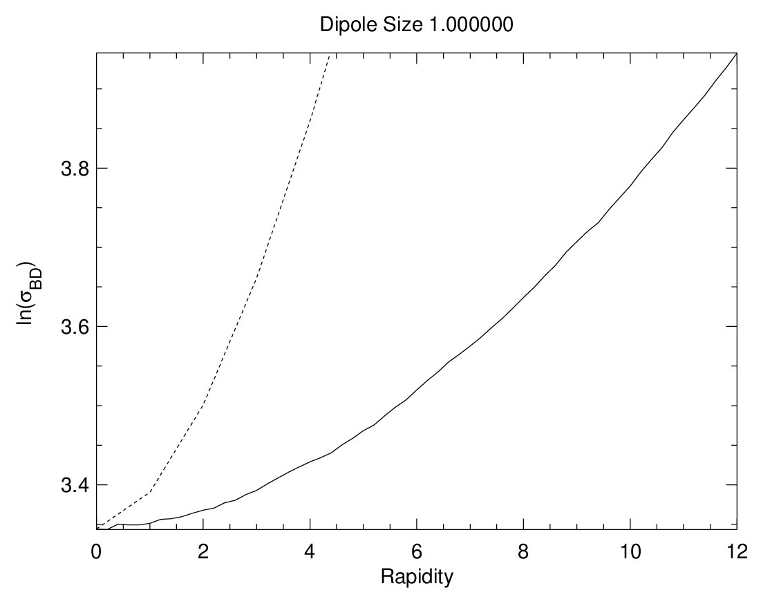
This black disc cross section is plotted in Fig. 13 and it can be seen that the slope of the black disc cross section in rapidity reaches a constant value at large rapidities. One can parametrize as
| (42) |
where is a normalization constant and is extracted from the numerical solutions in the regime where it is approximately constant. These extracted values for the solutions with two kernels as well as various values of are found in Table 2. The table also shows that with changing the exponent is relatively constant for the LO kernel, once again nonlinearities in the exponent appear for the Bessel kernel. Reported exponents are averaged from values of dipole size because does vary slightly with dipole size.


| LO Kernel | 2.4 |
| Modified Kernel | 2.0 |
| LO Kernel | 2.6 |
| Modified Kernel | 1.6 |
VI Including the running coupling
Turning now to the running of the QCD coupling, is taken to be where , is the number of active flavors and is used. In the infra-red regime, the coupling was frozen when which is defined as . As it is well known the BK equation without the impact parameter is not very sensitive to the way the coupling is regularized. This is because the amplitude is saturated for all the large values of the dipole size from the inverse of the saturation scale to infinity. In the case with impact parameter however, there are contributions from the large dipole regime which spoil this self-regularizing behavior. In this case there is a large sensitivity to the regularization scenario for the running coupling.
There are two different schemes for including the running coupling in the BK equation [65], [66]. In addition to these two scenarios we will use also the so-called parent dipole scheme, where the coupling depends on the size of the external dipole, that is . This scheme is convenient to use with the Bessel function kernel. We have also evaluated the solutions using the prescription proposed in [65]
| (43) |
Since it is not clear at the moment how to use this scheme with the Bessel function kernel we will use it only with the LO kernel. The scheme dependence between two prescriptions [65], [66] originates from the choice of the subtraction point. The scheme by [66] was shown to agree with the scheme [65] by the calculation of the appropriate subtraction corrections. In this paper we have not evaluated the scheme [66], as we have found that in order to achieve the desired accuracy for the solution with impact parameter within this scheme takes considerably longer time.
We first shall show the results with the running coupling without the impact parameter. The running of the coupling has the effect of slowing down the evolution of the scattering amplitude as seen in Fig.14. The difference between the LO and the modified kernel with running coupling is rather small. This can also be seen in Fig.15 which shows the saturation scale of the two kernels with running coupling which are extremely close to each other.


The dependence on the saturation scale with respect to the rapidity is as in [54]
| (44) |
where . Here the second term involving is numerically non-negligible for the rapidities we consider. In terms of numbers the coefficients above give We have found that the LO saturation scale with running coupling and the parent dipole size prescription is which is very similar to the one given by the analytical value. The running coupling with prescription (43) has also been run and found to have a fit of which is closer to the value given by (44).

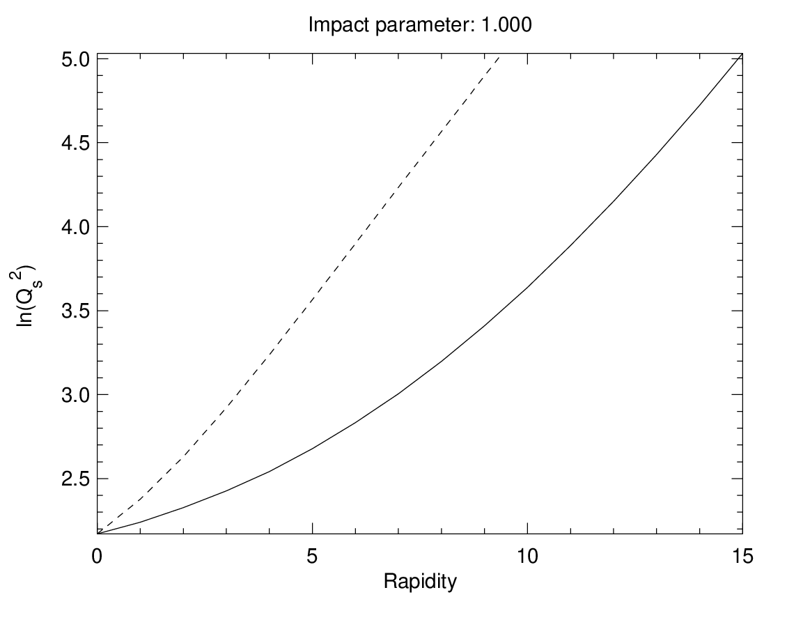
In the scenario with impact parameter we find quite different behavior of the solution. As is seen in Fig. 16 the evolution of the running coupling (with parent dipole scheme) is actually very fast in the small dipole region, and it is much faster in the large dipole region. This is obvious since in the large dipole region the coupling is fixed at which yields approximately three times as fast an evolution versus the case where is fixed. It can be seen there are box effects beginning to manifest in the running coupling case due to the frozen coupling evolving very quickly in the large dipole regime and reaching the box.
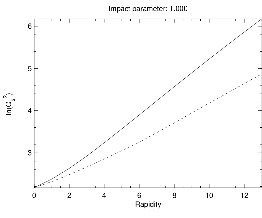
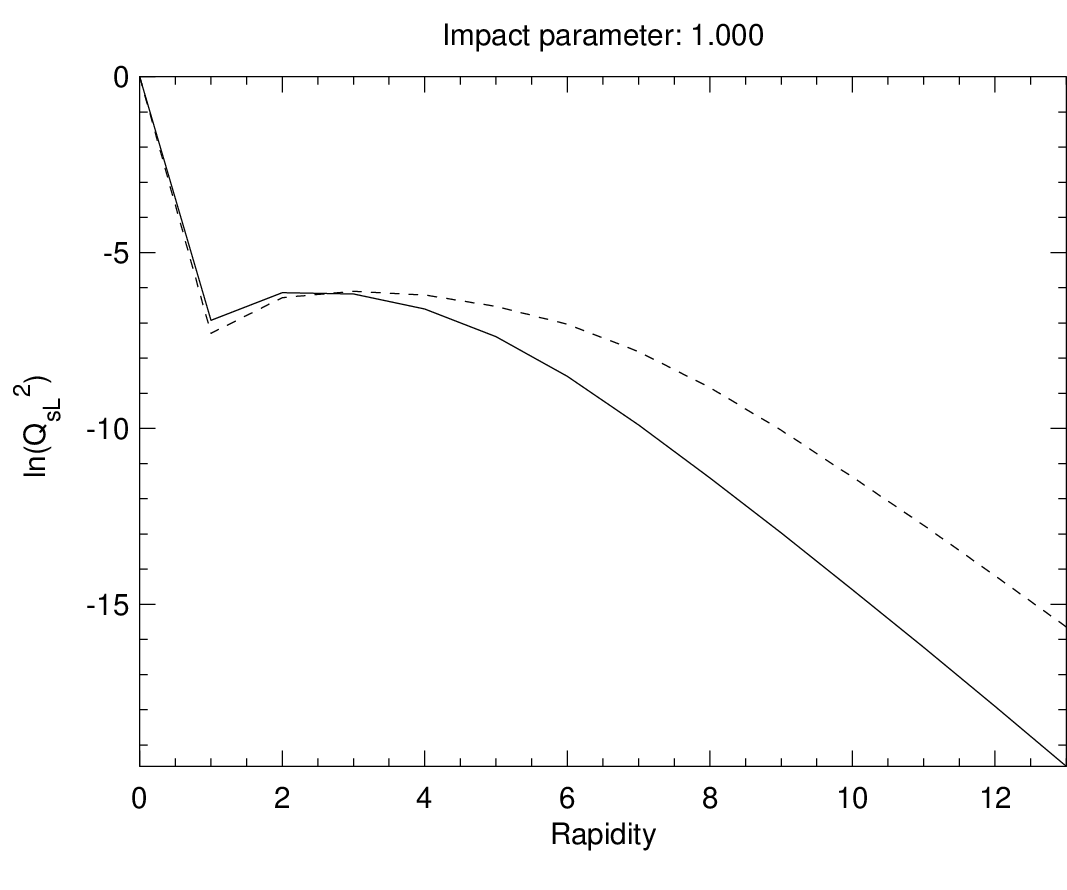
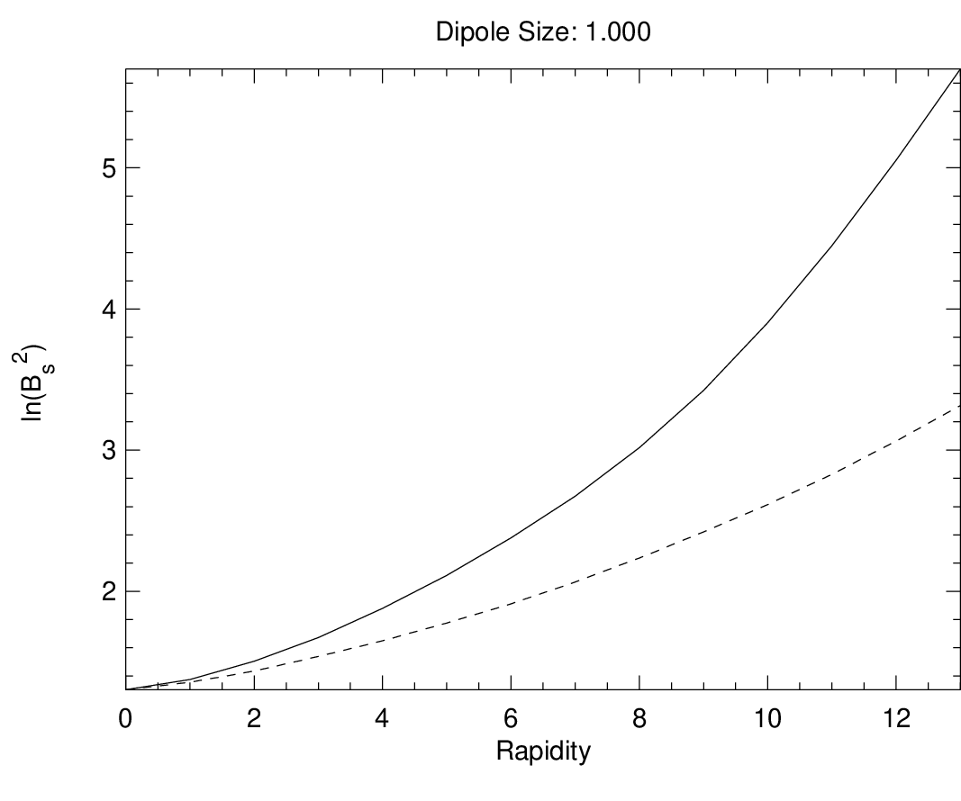
It can be seen in Fig. 17 that the dependence of the saturation scales on the rapidity is now again almost exponential. In this case we can extract the exponents by fitting exponential forms in the rapidity as we did for the fixed coupling case (table 3). Note that the definition of the exponents are now different than in the previous section. Here, we took . The reason that the dependencies are almost exponential is due to the large sensitivity to the infrared and the fact that the coupling is frozen. In that case the solutions behave as almost with the fixed running determined by the freezing value.
Similar pattern is found in the case of the running coupling with the scenario (43). The only difference is in the small dipole regime where the evolution is slightly slower than that of the parent dipole scheme. This can be seen by comparing the extracted exponents in Table 3.
| LO Kernel | 0.30 | 1.68 | 0.60 | 0.65 |
|---|---|---|---|---|
| LO Kernel | 0.29 | 1.68 | 0.64 | 0.68 |
| Bessel Kernel | 0.22 | 1.42 | 0.24 | 0.32 |

The behavior observed is of course something that has been analyzed before, in the context of the linear BFKL with running coupling [67]. In particular it was observed that, the BFKL solution shows the tunneling scenario, where at some value of rapidity the solution is completely dominated by the infrared region. Strictly speaking we are not observing the tunneling scenario here, due to the fact that we have chosen our initial conditions to be concentrated around rather large dipole sizes where the coupling is already large. Rather, our solutions are completely dominated by the large coupling values and hence the saturation scale has nearly exponential dependence on rapidity. It will be interesting to analyze the solution for the initial conditions which are located in the small dipole regime to see if the tunneling occurs here.
We have also evaluated the dipole cross section coming from the black disc regime in the running coupling scenario, and we parametrize it in the form
| (45) |
The extracted value for the exponent is shown also in Table3. Again the black disc cross section increases very fast due to the large value of the coupling in the region of freezing. We have also compared the solutions in the case of the LO and Bessel kernel, the results are shown in Fig. 18. Since the coupling is relatively large, the differences between the evolution with LO and Bessel kernels are more amplified.
VII Conclusions
Let us summarize the most important points of our analysis.
In the case of the solution with the LO kernel, the extracted exponents of the saturation scales and the black disc radius are consistent with values obtained from the boundary method. The peaks in impact parameter and in dipole size can be very easily understood from arguments based on the conformal symmetry. The relative strength of the evolution of different saturation scales follows as well from the arguments on the conformal symmetry. In particular the black disc radius has an expansion rate which is twice slower than that of the saturation scale for small dipoles.
For the running coupling scenario, in the case of the solutions with impact parameter we no longer observe the self-regularizing behavior of the nonlinear equation. This is of course due to the increased sensitivity to the large values of the dipole size. Rather, for the initial conditions chosen one observes strong dependence on the details of the regularization, and basically the exponents of both the saturation scales are dominated by the largest value of the coupling. This could be tested in more detail by choosing different initial condition, nevertheless one can expect that for the sufficiently large rapidity, the solution becomes regularization-sensitive, much like it was observed in earlier simulations.
The cuts on the large dipole sizes, introduced in the form of the modified kernel have in general very small effect for the case of the impact parameter independent kernel. For the case with the impact parameter they are no longer negligible and reduce the exponent by about for coupling of . It is important to note that, the modified kernel we have chosen does not account for all the type of kinematical cuts, and therefore other cuts, on the small dipole sizes should be included similarly to what was done in [50]. One could expect therefore even stronger effect in this case.
We therefore conclude that the observed self-regularizing behavior of the local BK equation with the running coupling and almost complete insensitivity to the other NLO corrections appear due to the simplified assumption about the impact parameter independence.
In a broader perspective, it will be interesting to perform the analysis with full NLO kernel or the more correct form of the kinematical cuts, as well as introduce effectively confinement effects. It is also vital to analyze the impact of the corrections which go beyond the mean field approximation [68, 69, 62, 70].
Acknowledgments
We would like to thank Emil Avsar and Leszek Motyka for interesting discussions. This work was supported by the MNiSW grant No. N202 249235 and the DOE OJI grant No. DE - SC0002145. A.M.S. is supported by the Sloan Foundation.
References
- [1] V. S. Fadin, E. A. Kuraev and L. N. Lipatov, Phys. Lett. B60, 50 (1975).
- [2] E. A. Kuraev, L. N. Lipatov and V. S. Fadin, Sov. Phys. JETP 45, 199 (1977).
- [3] I. I. Balitsky and L. N. Lipatov, Sov. J. Nucl. Phys. 28, 822 (1978).
- [4] L. N. Lipatov, Sov. Phys. JETP 63, 904 (1986).
- [5] V. S. Fadin and L. N. Lipatov, Nucl. Phys. B477, 767 (1996), [hep-ph/9602287].
- [6] V. S. Fadin, M. I. Kotsky and L. N. Lipatov, hep-ph/9704267.
- [7] V. S. Fadin and L. N. Lipatov, Phys. Lett. B429, 127 (1998), [hep-ph/9802290].
- [8] M. I. Kotsky, V. S. Fadin and L. N. Lipatov, Phys. Atom. Nucl. 61, 641 (1998).
- [9] G. Camici and M. Ciafaloni, Phys. Lett. B386, 341 (1996), [hep-ph/9606427].
- [10] G. Camici and M. Ciafaloni, Phys. Lett. B395, 118 (1997), [hep-ph/9612235].
- [11] G. Camici and M. Ciafaloni, Phys. Lett. B412, 396 (1997), [hep-ph/9707390].
- [12] G. Camici and M. Ciafaloni, Nucl. Phys. Proc. Suppl. 54A, 155 (1997).
- [13] M. Ciafaloni and G. Camici, Phys. Lett. B430, 349 (1998), [hep-ph/9803389].
- [14] L. V. Gribov, E. M. Levin and M. G. Ryskin, Phys. Rept. 100, 1 (1983).
- [15] Y. V. Kovchegov, Phys. Rev. D60, 034008 (1999), [hep-ph/9901281].
- [16] Y. V. Kovchegov, Phys. Rev. D61, 074018 (2000), [hep-ph/9905214].
- [17] A. H. Mueller, Nucl. Phys. B415, 373 (1994).
- [18] I. Balitsky, Nucl. Phys. B463, 99 (1996), [hep-ph/9509348].
- [19] I. Balitsky, Phys. Rev. Lett. 81, 2024 (1998), [hep-ph/9807434].
- [20] I. Balitsky, Phys. Rev. D60, 014020 (1999), [hep-ph/9812311].
- [21] I. Balitsky, Phys. Lett. B518, 235 (2001), [hep-ph/0105334].
- [22] I. I. Balitsky and A. V. Belitsky, Nucl. Phys. B629, 290 (2002), [hep-ph/0110158].
- [23] J. Jalilian-Marian, A. Kovner and H. Weigert, Phys. Rev. D59, 014015 (1999), [hep-ph/9709432].
- [24] J. Jalilian-Marian, A. Kovner, A. Leonidov and H. Weigert, Phys. Rev. D59, 014014 (1999), [hep-ph/9706377].
- [25] E. Iancu, A. Leonidov and L. D. McLerran, Nucl. Phys. A692, 583 (2001), [hep-ph/0011241].
- [26] E. Iancu, A. Leonidov and L. D. McLerran, Phys. Lett. B510, 133 (2001), [hep-ph/0102009].
- [27] E. Ferreiro, E. Iancu, A. Leonidov and L. McLerran, Nucl. Phys. A703, 489 (2002), [hep-ph/0109115].
- [28] H. Weigert, Nucl. Phys. A703, 823 (2002), [hep-ph/0004044].
- [29] A. H. Mueller, Phys. Lett. B523, 243 (2001), [hep-ph/0110169].
- [30] J. Bartels, Z. Phys. C60, 471 (1993).
- [31] J. Bartels and M. Wusthoff, Z. Phys. C66, 157 (1995).
- [32] J. Bartels, L. N. Lipatov and G. P. Vacca, Nucl. Phys. B706, 391 (2005), [hep-ph/0404110].
- [33] M. Lublinsky, Eur. Phys. J. C21, 513 (2001), [hep-ph/0106112].
- [34] M. Lublinsky, E. Gotsman, E. Levin and U. Maor, Nucl. Phys. A696, 851 (2001), [hep-ph/0102321].
- [35] K. J. Golec-Biernat, L. Motyka and A. M. Stasto, Phys. Rev. D65, 074037 (2002), [hep-ph/0110325].
- [36] N. Armesto and M. A. Braun, Eur. Phys. J. C20, 517 (2001), [hep-ph/0104038].
- [37] M. A. Braun, hep-ph/0101070.
- [38] A. H. Mueller and D. N. Triantafyllopoulos, Nucl. Phys. B640, 331 (2002), [hep-ph/0205167].
- [39] J. Bartels and K. Kutak, Eur. Phys. J. C53, 533 (2008), [0710.3060].
- [40] J. Bartels, L. N. Lipatov and M. Wusthoff, Nucl. Phys. B464, 298 (1996), [hep-ph/9509303].
- [41] K. J. Golec-Biernat and A. M. Stasto, Nucl. Phys. B668, 345 (2003), [hep-ph/0306279].
- [42] E. Gotsman, M. Kozlov, E. Levin, U. Maor and E. Naftali, Nucl. Phys. A742, 55 (2004), [hep-ph/0401021].
- [43] L. Motyka and A. M. Stasto, Phys. Rev. D79, 085016 (2009), [0901.4949].
- [44] J. Kwiecinski, A. D. Martin and P. J. Sutton, Z. Phys. C71, 585 (1996), [hep-ph/9602320].
- [45] A. Kormilitzin and E. Levin, 1009.1468.
- [46] G. Chachamis, M. Lublinsky and A. Sabio Vera, Nucl. Phys. A748, 649 (2005), [hep-ph/0408333].
- [47] I. Balitsky and G. A. Chirilli, Phys. Rev. D77, 014019 (2008), [0710.4330].
- [48] E. Avsar, G. Gustafson and L. Lonnblad, JHEP 01, 012 (2007), [hep-ph/0610157].
- [49] I. Balitsky and G. A. Chirilli, Phys. Lett. B687, 204 (2010), [0911.5192].
- [50] E. Avsar, G. Gustafson and L. Lonnblad, JHEP 07, 062 (2005), [hep-ph/0503181].
- [51] A. H. Mueller, Nucl. Phys. B558, 285 (1999), [hep-ph/9904404].
- [52] A. H. Mueller, hep-ph/9911289.
- [53] C. Marquet and G. Soyez, Nucl. Phys. A760, 208 (2005), [hep-ph/0504080].
- [54] S. Munier and R. B. Peschanski, Phys. Rev. D69, 034008 (2004), [hep-ph/0310357].
- [55] G. P. Salam, JHEP 07, 019 (1998), [hep-ph/9806482].
- [56] M. Ciafaloni, D. Colferai, G. P. Salam and A. M. Stasto, Phys. Rev. D68, 114003 (2003), [hep-ph/0307188].
- [57] A. Sabio Vera, Nucl. Phys. B722, 65 (2005), [hep-ph/0505128].
- [58] E. Avsar, Acta Phys. Polon. B37, 3561 (2006), [hep-ph/0610045].
- [59] E. Avsar, JHEP 11, 027 (2007), [0709.1371].
- [60] M. Ryskin, Talk at DIS2003 conference. .
- [61] H. Navelet and S. Wallon, Nucl. Phys. B522, 237 (1998), [hep-ph/9705296].
- [62] Y. Hatta and A. H. Mueller, Nucl. Phys. A789, 285 (2007), [hep-ph/0702023].
- [63] A. Kovner and U. A. Wiedemann, Phys. Lett. B551, 311 (2003), [hep-ph/0207335].
- [64] A. Kovner and U. A. Wiedemann, Phys. Rev. D66, 051502 (2002), [hep-ph/0112140].
- [65] I. Balitsky, Phys. Rev. D75, 014001 (2007), [hep-ph/0609105].
- [66] Y. V. Kovchegov and H. Weigert, Nucl. Phys. A784, 188 (2007), [hep-ph/0609090].
- [67] M. Ciafaloni, D. Colferai, G. P. Salam and A. M. Stasto, Phys. Lett. B541, 314 (2002), [hep-ph/0204287].
- [68] A. H. Mueller and G. P. Salam, Nucl. Phys. B475, 293 (1996), [hep-ph/9605302].
- [69] A. H. Mueller and A. I. Shoshi, Nucl. Phys. B692, 175 (2004), [hep-ph/0402193].
- [70] A. H. Mueller and S. Munier, Phys. Rev. D81, 105014 (2010), [1002.4575].