Spin and Magnetization Effects in Plasmas

The basic equation of nonrelativistic quantum mechanics is the Schrödinger equation. The dynamics of an electron, represented by its wave function $\psi$, in an external electromagnetic potential $\phi$ is governed by

$$i\hbar\frac{\partial\psi}{\partial t}+\frac{\hbar}{2m_{e}}\nabla^{2}\psi+e\phi\psi=0,$$

(1)

where $\hbar$ is Planck’s constant, $m_{e}$ is the electron mass, and $e$ is the magnitude of the electron charge. This complex equation may be written as two real equations, writing $\psi=\sqrt{n}\,\exp{iS/\hbar}$, where $n$ is the amplitude and $S$ the phase of the wave function, respectively [2]. Such a decomposition was presented by de Broglie and Bohm in order to understand the dynamics of the electron wave packet in terms of classical variables. Using this decomposition in Eq. (1), we obtain

$$\frac{dn}{dt}=-n\nabla\cdot\mathbf{v},$$

(2)

and

$$m_{e}\frac{d\mathbf{v}}{dt}=e\nabla\phi+\frac{\hbar^{2}}{2m_{e}}\nabla\left(\frac{\nabla^{2}\sqrt{n}}{\sqrt{n}}\right),$$

(3)

where the velocity is defined by $\mathbf{v}=\nabla S/m_{e}$ and $d/dt=\partial_{t}+\mathbf{v}\cdot\nabla$. The last term of Eq. (3) is the gradient of the Bohm–de Broglie potential, and is due to the effect of wave function spreading, giving rise to a dispersive-like term. We also note the striking resemblance of Eqs. (2) and (3) to the classical fluid equations.

The non-relativistic evolution of spin-1/2 particles, as described by the two-component spinor $\varPsi_{(\alpha)}$, is given by the Pauli equation (see, e.g., [2])

$$i\hbar\frac{\partial\psi}{\partial t}+\left[\frac{\hbar^{2}}{2m_{e}}\left(\nabla+\frac{ie}{\hbar}\mathbf{A}\right)^{2}-\mu_{B}\mathbf{B}\cdot\mathbf{\sigma}+e\phi\right]\psi=0,$$

(4)

where $\mathbf{A}$ is the vector potential, $\mu_{B}=e\hbar/2m_{e}$ is the Bohr magneton, and $\mathbf{\sigma}=(\sigma_{1},\sigma_{2},\sigma_{3})$ is the Pauli spin vector.

Now, in the same way as in the Schrödinger case, we may decompose the electron wave function $\psi$ into its amplitude and phase. However, as the electron has spin, the wave function is now represented by a 2-spinor instead of a c-number. Thus, we may use $\psi=\sqrt{n}\,\exp(iS/\hbar)\varphi$, where $\varphi$, normalized such that $\varphi^{{\dagger}}\varphi=1$, now gives the spin part of the wave function. Multiplying the Pauli equation (4) by $\psi^{{\dagger}}$, inserting the above wave function decomposition and taking the gradient of the resulting phase evolution equation, we obtain the conservation equations

$$\frac{dn}{dt}=-n\nabla\cdot\mathbf{v}$$

(5)

and

	$\displaystyle\frac{dv_{i}}{dt}$	$\displaystyle=$	$\displaystyle-\frac{e}{m_{e}}(E_{i}+\epsilon_{ijk}v_{j}B_{k}+\frac{\hbar^{2}}{2m_{e}^{2}}\frac{\partial}{\partial x_{i}}\left(\frac{\nabla^{2}\sqrt{n}}{\sqrt{n}}\right)$		(6)
			$\displaystyle-\frac{\mu_{B}}{m_{e}}s_{j}\frac{\partial B_{j}}{\partial x_{i}}-\frac{\hbar^{2}}{4m_{e}^{2}n}\frac{\partial}{\partial x_{j}}\left(n\Gamma_{ij}\right)$

respectively, where $\epsilon_{ijk}$ is the fully antisymmetric (pseudo-)tensor and we have used Einstein’s sum convention so that a sum over indices occurring twice in a term is implied, where $i,j,k,\dots=1,2,3$. The spin contribution to Eq. (6) is consistent with the results of Ref. [15]. Here the velocity is defined by

$$\mathbf{v}=\frac{1}{m_{e}}\left({\nabla}S-i\hbar\varphi^{{\dagger}}\mathbf{\nabla}\varphi\right)+\frac{e\mathbf{A}}{m_{e}c},$$

(7)

the spin density vector is

$$\mathbf{s}=\varphi^{{\dagger}}\mathbf{\sigma}\varphi,$$

(8)

which is normalized according to¹¹ 1 An alternative choice for the normalization would be to choose $|\mathbf{s}|=\hbar/2$.

$$|\mathbf{s}|=1,$$

(9)

and we have defined the symmetric gradient spin tensor

$$\Gamma_{ij}=\frac{\partial s_{k}}{\partial x_{i}}\frac{\partial s_{k}}{\partial x_{j}}.$$

(10)

Moreover, contracting Eq. (4) by $\psi^{{\dagger}}\mathbf{\sigma}$, we obtain the spin evolution equation

$\displaystyle\frac{ds_{i}}{dt}=\epsilon_{ijk}\left\{\frac{2\mu_{B}}{\hbar}B_{j}-\frac{\hbar}{2m_{e}n}\left[\frac{\partial}{\partial x_{l}}\left(n\frac{\partial s_{j}}{\partial x_{l}}\right)\right]\right\}s_{k}.$

(11)

We note that the last equation allows for the introduction of an effective magnetic field $\mathbf{B}_{\mathrm{eff}}\equiv({2\mu_{B}}/{\hbar})\mathbf{B}-\hbar/\left[\partial_{j}(n\partial_{j}\mathbf{s})\right]/(2m_{e}n)$. However, this will not pursued further here (for a discussion, see Ref. [2]).

Comparing the effects due to spin from the Pauli dynamics with the Schrödinger theory, we see a significant increase in the complexity of the fluid like equations due the presence of spin. The fact that the spin couples linearly to the magnetic field makes the dynamical aspects of such Pauli systems very rich. Moreover, when going over to the collective regime, the back reaction through Maxwell’s equation can yield interesting new properties of such spin plasmas. In fact, the introduction of an intrinsic magnetization can give rise to linear instability regimes, much like the Jeans instability.

As pointed out in the previous section, the route from single wavefunction dynamics to collective effects introduces a new complexity into the system. At the classical level, the ordinary pressure is such an effect. In the quantum case, a similar term, based on the thermal distribution of spins, will be introduced.

The concept of a magnetoplasma was first introduced in the pioneering work [16] by Alfvén, who showed the existence of waves in magnetized plasmas. Since then, magnetohydrodynamics (MHD) has found applications in a vast range of fields, from solar physics and astrophysical dynamos, to fusion plasmas and dusty laboratory plasmas.

Magnetic fields, an essential component in the MHD description of plasmas, also couples directly to the spin of the electron. Thus, the presence of spin alters the single electron dynamics, introducing a correction to the Lorentz force term. Indeed, from the experimental perspective, a certain interest has been directed towards the relation of spin properties to the classical theory of motion (see, e.g., Refs. [17, 18, 19, 20, 21, 22, 23, 24, 25, 26, 27, 28, 29]). In particular, the effects of strong fields on single particles with spin has attracted experimental interest in the laser community [19, 20, 21, 22, 23, 25]. However, the main objective of these studies was single particle dynamics, relevant for dilute laboratory systems, whereas our focus will be on collective effects.

We will now include if the ion species, which are assumed to be described by the classical equations and have charge $Ze$, we may derive a set of one- fluid equations [14]. The ion equations read

$$\frac{dn_{I}}{dt}=-n_{I}\nabla\cdot\mathbf{v}_{I},$$

(32)

and

$$m_{I}n_{I}\frac{dv_{Ii}}{dt}=Zen_{I}\left(E_{i}+\epsilon_{ijk}v_{Ij}B_{k}\right)-\frac{\partial p_{I}}{\partial x_{i}},$$

(33)

Next we define the total mass density $\rho\equiv(m_{e}n+m_{I}n_{I})$, the centre-of-mass fluid flow velocity $\mathbf{V}\equiv(m_{e}n\mathbf{v}_{e}+m_{I}n_{I}\mathbf{v}_{I})/\rho$, and the current density $\mathbf{j}=-en\mathbf{v}_{e}+Zen_{I}\mathbf{v}_{I}$. Using these denfinitions, we immediately obtain

$$\frac{d\rho}{dt}=-\rho\nabla\cdot\mathbf{V},$$

(34)

from Eqs. (21) and (32). Assuming quasi-neutrality, i.e. $n\approx Zn_{I}$, the momentum conservation equations (25) and (33) give

$$\rho\frac{dV_{i}}{dt}=\epsilon_{ijk}j_{j}B_{k}-\frac{\partial\mathsf{\Pi}_{ij}}{\partial x_{j}}-\frac{\partial p}{\partial x_{i}}+\frac{Z\hbar^{2}\rho}{2m_{e}m_{I}}\frac{\partial}{\partial x_{i}}\left(\frac{\nabla^{2}\sqrt{\rho}}{\sqrt{\rho}}\right)+F^{\text{spin}}_{i},$$

(35)

where $\mathbf{\mathsf{\Pi}}$ is the tracefree pressure tensor in the centre-of-mass frame, and $P$ is the scalar pressure in the centre-of-mass frame. We also note that due to quasi-neutrality, we have $n_{e}\approx Z\rho/m_{I}$ and $\mathbf{v}=\mathbf{V}-m_{I}\mathbf{j}/Ze\rho$, and we can thus express the quantum terms in terms of the total mass density $\rho$, the centre-of-mass fluid velocity $\mathbf{V}$, and the current $\mathbf{j}$. With this, the spin transport equation (26) reads

$$\rho\frac{dS_{i}}{dt}=\frac{m_{e}}{Ze}j_{j}\frac{\partial S_{i}}{\partial x_{j}}+\frac{2\mu_{B}\rho}{\hbar}\epsilon_{ijk}B_{j}S_{k}-\frac{m_{I}}{Z}\frac{\partial\Sigma_{ij}}{\partial x_{j}}+\frac{m_{I}}{Z}\Omega^{\text{spin}}.$$

(36)

In the momentum equation (35), neglecting the pressure and the Bohm–de Broglie potential for the sake of clarity, we have the force density $\mathbf{j}\times\mathbf{B}+\mathbf{F}_{\text{spin}}$. In general, for a magnetized medium with magnetization density $\mathbf{M}$, Ampère’s law gives the free current in a finite volume $V$ according to

$$\mathbf{j}=\frac{1}{\mu_{0}}\mathbf{\nabla}\times\mathbf{B}-\mathbf{\nabla}\times\mathbf{M},$$

(37)

where we have neglected the displacement current. The surface current is an important part of the total current when we are interested in the forces on a finite volume, as was demonstrated in Ref. [14] and will be shown below.

It it worth noting that the expression of the force density in the momentum conservation equation can, to lowest order in the spin, be derived on general macroscopic grounds. Formally, the total force density on a volume element $V$ is defined as $\mathbf{F}=\lim_{V\rightarrow 0}(\sum_{\alpha}\mathbf{f}_{\alpha}/V)$, where $\mathbf{f}_{\alpha}$ are the different forces acting on the volume element, and might include surface forces as well. For magnetized matter, the total force on an element of volume $V$ is then

$$\mathbf{f}_{\mathrm{tot}}=\int_{V}\mathbf{j}_{\mathrm{tot}}\times\mathbf{B}\,\mathrm{d}V+\oint_{\partial V}(\mathbf{M}\times\hat{\mathbf{n}})\times\mathbf{B}\,\mathrm{d}S$$

(38)

where (neglecting the displacement current) $\mathbf{j}_{\mathrm{tot}}=\mathbf{j}+\mathbf{\nabla}\times\mathbf{M}$. Inserting the expression for the total current into the volume integral and using the divergence theorem on the surface integral, we obtain the force density

$$\mathbf{F}_{\mathrm{tot}}=\mathbf{j}\times\mathbf{B}+M_{k}\mathbf{\nabla}B^{k},$$

(39)

identical to the lowest order description from the Pauli equation (see Eq. (35)). Inserting the free current expression (37), due to Ampère’s law, we can write the total force density according to

$${F}^{i}=-\partial^{i}\left(\frac{B^{2}}{2\mu_{0}}-\mathbf{M}\cdot\mathbf{B}\right)+\partial_{k}({H^{i}B^{k}}).$$

(40)

The first gradient term in Eq. (40) can be interpreted as the force due to a potential (the energy of the magnetic field and the magnetization vector in that field), while the second divergence term is the anisotropic magnetic pressure effect. Noting that the spatial part of the stress tensor takes the form [15]

$$T^{ik}=-H^{i}B^{k}+(B^{2}/2\mu_{0}-\mathbf{M}\cdot\mathbf{B})\delta^{ik},$$

(41)

we see that the total force density on the magnetized fluid element can be written $F^{i}=-\partial_{k}T^{ik}$, as expected. Thus, the Pauli theory results in the same type of conservation laws as the macroscopic theory. The momentum conservation equation (35) then reads

$$\rho\left(\frac{\partial}{\partial t}+\mathbf{V}\cdot\mathbf{\nabla}\right)\mathbf{V}=-\mathbf{\nabla}\left(\frac{B^{2}}{2\mu_{0}}-\mathbf{M}\cdot\mathbf{B}\right)+B^{k}\partial_{k}\mathbf{H}-\mathbf{\nabla}p,$$

(42)

where for the sake of clarity we have assumed an isotropic pressure, dropped the displacement current term in accordance with the nonrelativistic assumption, and neglected the Bohm potential (these terms can of course simply be added to (42)). This concludes the discussion of the spin-MHD plasma case. Next, we will look at some applications of the derived equations. However, it should be noted that in many cases the spins are close to thermodynamic equilibrium, and we can thus write the paramagnetic electron response in terms of the magnetization [14]

$$\mathbf{M}=\frac{\mu_{B}\rho}{m_{I}}\,\tanh\left(\frac{\mu_{B}B}{k_{B}T}\right)\widehat{\mathbf{B}},$$

(43)

instead of using the full spin dynamics. Here $B$ denotes the magnitude of the magnetic field and $\widehat{\mathbf{B}}$ is a unit vector in the direction of the magnetic field, $k_{B}$ is Boltzmann’s constant, and $T$ is the electron temperature.

The distribution function which we will work with here is the combination of the Wigner distribution function [7] for the phase-space variables and the q-function for the spin degree of freedom [47]. This combination of distribution functions was used in [49] and it turns out to yield a intuitive description of spin-1/2 particles in an extended phase space.

Given a 2-by-2 density matrix (in the Schrödinger pricture $\rho(\mathbf{x},\mathbf{y},t)$ for a spin particle the extended phase-space distribution function is defined by

$$f(\mathbf{x},\mathbf{p},\mathbf{s},t)=\frac{1}{4\pi}\mathrm{Tr}\left[\left(1+\mathbf{s}\cdot\bm{\sigma}\right)W(\mathbf{x},\mathbf{p},t)\right],$$

(44)

where $\mathrm{Tr}$ denotes that the trace is to be calculated of the resulting 2-by-2 matrix and where $\bm{\sigma}$ is a vector with the Pauli matrices as components, $\mathbf{s}$ is a vector on the unit sphere. The Wigner distribution matrix function is given by

$$W(\mathbf{x},\mathbf{p},t)=\int\frac{d^{3}y}{(2\pi\hbar)^{3}}e^{-\frac{i}{\hbar}\mathbf{y}\cdot\left[\mathbf{p}+iq\int_{-1/2}^{1/2}ds\mathbf{A}(\mathbf{x}+s\mathbf{y},t)\right]}\rho\left(\mathbf{x}+\frac{\mathbf{y}}{2};\mathbf{x}-\frac{\mathbf{y}}{2},t\right),$$

(45)

where $q$ is the charge of the particle and $\mathbf{A}$ is the vector potential. The integral over the vector potential is there to ensure gauge invariance. The momentum variable $\mathbf{p}$ is the gauge invariant kinetic momentum related to the canonical momentum $\mathbf{p}_{c}$ by $\mathbf{p}=\mathbf{p}_{c}-q\mathbf{A}(\mathbf{x},t)$. This distribution function is defined on an extended phase-space $(\mathbf{x},\mathbf{p},\mathbf{s})$ and can in principle be used to calculate the expectation value of any observable defined by an operator $\hat{O}=O(\hat{\mathbf{x}},\hat{\mathbf{p}},\bm{\sigma})$. The way to do this is to use the modified Weyl correspondence [44] together with a transformation for the spin variable to obtain a phase-space function, and subsequently take the average of this function weighted by the distribution function. For an operator depending on $\hat{\mathbf{x}},\hat{\mathbf{p}}$ the corresponding phase-space function is obtained by

$$O(\mathbf{x},\mathbf{p})=\int d^{3}ye^{-\frac{i}{\hbar}\mathbf{y}\cdot\left[\mathbf{p}+q\int_{-1/2}^{1/2}ds\mathbf{A}(\mathbf{x}+s\mathbf{y},t)\right]}\left\langle\mathbf{x}+\frac{\mathbf{y}}{2}\right|\hat{O}\left|\mathbf{x}-\frac{\mathbf{y}}{2}\right\rangle$$

(46)

It can sometimes be found more easily by first putting the position and kinetic momentum operators of the operator $\hat{O}$ in symmetric order using the commutation relation and then make the substitution $\hat{\mathbf{x}}\rightarrow\mathbf{x}$ and $\hat{\mathbf{p}}\rightarrow\mathbf{p}$. For example the pressure tensor which just contains the kinetic momentum operator is obtained by $\hat{P}_{ij}=\hat{p}_{i}\hat{p}_{j}\rightarrow p_{i}p_{j}$. Note that the gauge dependent Wigner distribution this correspondence is not so simple anymore, since we are then dealing with the position and canonical momentum operators which has to be ordered symmetrically using the commutation relation. So for the moment above, for example we have to put the combination $\hat{P}_{ij}=[\hat{p}_{ci}-qA_{i}(\hat{\mathbf{x}})][\hat{p}_{cj}-qA_{j}(\hat{\mathbf{x}})]$ in symmetric ordering and then make the substitution $\hat{x}_{i}\rightarrow x_{i}$ and $\hat{p}_{i}\rightarrow p_{i}$. This is a quite difficult task for a general operator since the form of the vector potential is not necessarily known.

The spin space function corresponding an operator $\hat{O}$ depending on $\bm{\sigma}$ is obtained by transformation

$$O(\mathbf{s})=\frac{1}{4\pi}\mathrm{Tr}\left[\left(1+\mathbf{s}\cdot\bm{\sigma}\right)\hat{O}\right].$$

(47)

If the operator in question depends on both the position and momentum operators and the spin, both of these transformations have to be made, see Ref. . Since $\bm{\sigma}^{2}=1$ the only possible spin operators we may have is the identity operator 1 and $\bm{\sigma}$. The transformation (47) above yields

$$\hat{O}=\bm{\sigma}\rightarrow O(\mathbf{s})=3\mathbf{s}.$$

(48)

The momentum variable in the Wigner function above is the canonical momentum. In the presence of a magnetic field it is often more convenient to work with the gauge invariant kinetic momentum.

The Hamiltonian for a spin-1/2 particle in a magnetic field is given by

$$\hat{H}=\frac{[\hat{\mathbf{p}}_{c}-A(\hat{\mathbf{x}},t)]^{2}}{2m}+qV+\mu_{B}\bm{\sigma}\cdot\mathbf{B}(\hat{\mathbf{x}},t),$$

(49)

where $V$ and $\mathbf{A}$ are the electromagnetic potentials, $\mathbf{B}=\nabla\times\mathbf{A}$ is the magnetic induction and $\mu_{B}$ is the magnetic moment of the particle. Specifically, for an electron, the magnetic moment is given by $\mu_{B}=qg\hbar/(4m)$ where $g\approx 2.001$ is a correction factor deduced from quantum electrodynamics [50]. Note that we have used $q=-|e|$ so that the magnetic moment is negative. The evolution equation for the density operator is given by the von Neumann equation

$$i\hbar\partial_{t}\rho=[\rho,\hat{H}].$$

(50)

Taking the transform (44) of this equation, it is possible to derive an evolution equation for the extended phase space Wigner function $f(\mathbf{x},\mathbf{p},\mathbf{s},t)$, see Ref. [49] and it is given by

	$\displaystyle\frac{\partial f}{\partial t}+(\mathbf{v}+\Delta\tilde{\mathbf{v}})\cdot\nabla_{x}f+\frac{q}{m}\left[\tilde{\mathbf{E}}+(\mathbf{v}+\tilde{\mathbf{v}})\times\tilde{\mathbf{B}})\right]\cdot\nabla_{v}f$
	$\displaystyle+\frac{\mu_{B}}{m}\nabla_{x}\left[(\mathbf{s}+\nabla_{s})\cdot\tilde{\mathbf{B}}\right]\cdot\nabla_{v}f+\frac{2\mu_{B}}{\hbar}(\mathbf{s}\times\tilde{\mathbf{B}})\cdot\nabla_{s}f$	$\displaystyle=$	$\displaystyle 0.$		(51)

where $\mathbf{v}=\mathbf{p}/m$ is the velocity and we have defined the operators

	$\displaystyle\tilde{\mathbf{E}}$	$\displaystyle=$	$\displaystyle\mathbf{E}(\mathbf{x})\int_{-1/2}^{1/2}ds\cos\left(\frac{\hbar s}{m}\overleftarrow{\nabla}_{x}\cdot\overrightarrow{\nabla}_{v}\right)$		(52)
	$\displaystyle\tilde{\mathbf{B}}$	$\displaystyle=$	$\displaystyle\mathbf{B}(\mathbf{x})\int_{-1/2}^{1/2}ds\cos\left(\frac{\hbar s}{m}\overleftarrow{\nabla}_{x}\cdot\overrightarrow{\nabla}_{v}\right)$		(53)
	$\displaystyle\Delta\tilde{\mathbf{v}}$	$\displaystyle=$	$\displaystyle\frac{q\hbar}{m^{2}}\mathbf{B}(\mathbf{x})\int_{-1/2}^{1/2}dss\sin\left(\frac{\hbar s}{m}\overleftarrow{\nabla}_{x}\cdot\overrightarrow{\nabla}_{v}\right)\cdot\nabla_{v}.$		(54)

Note the similarity of the equation above with the classical Vlasov equation. In order to compare it further we may consider the semiclassical limit which is applicable when the typical length scale is much shorter than the de Broglie wave length $\hbar/(mv)$, where $v$ is the typical velocity of the system. We may then expand the sine and cosine operators above. Keeping terms up to order $\hbar^{2}$ the resulting equation is

$$\frac{\partial f}{\partial t}+\mathbf{v}\cdot\nabla_{x}f+\frac{q}{m}\left[\mathbf{E}+\mathbf{v}\times\mathbf{B}\right]+\frac{\mu_{B}}{m}\nabla_{x}\left[(\mathbf{s}+\nabla_{s})\cdot\mathbf{B}\right]\cdot\nabla_{v}f+\frac{2\mu_{B}}{\hbar}(\mathbf{s}\times\mathbf{B})\cdot\nabla_{s}f=0.$$

(55)

The first term proportional to the spin $\mathbf{s}$ is the dipole force of a magnetic moment in an inhomogeneous magnetic field and the last term is accounts for the spin precession. Both of these can be understood from a classical analog, however, there is also a quantum dipole term given by $(\mu_{B}/m)\nabla_{x}(\mathbf{B}\cdot\nabla_{s})\cdot\nabla_{v}f$. This term accounts for the fact that the spin is not a classical dipole and we can for example not have a distribution function proportional to $\delta(\mathbf{s}-\hat{z})$, where $\hat{z}$ is a unit vector in the z-direction. The corresponding distribution function in the quantum mechanical case is proportional to $1+\cos\theta_{s}$ where $\theta_{s}$ is the angle between the spin direction and the z-axis. The macroscopic magnetization the classical and quantum cases are still the same which is ensured by the factor 3 in the transformation (48) above. This factor occurs in the quantum case

$$\mathbf{M}_{\text{q}}(\mathbf{x})=3\mu_{B}\int d\Omega f(\mathbf{x},\mathbf{v},\mathbf{s}),$$

(56)

but is absent in the corresponding classical equation

$$\mathbf{M}_{\text{cl}}(\mathbf{x})=\mu_{B}\int d\Omega\mathbf{s}f_{\text{cl}}(\mathbf{x},\mathbf{v},\mathbf{s}),$$

(57)

where $f_{\text{cl}}$ is the classical distribution function and we in both cases have $d\Omega=d^{3}vd^{2}s$.

A semi classical version of Eq. (55) (where the quantum dipole term is missing) has been applied to find a new type of resonance due to radiative corrections to the electron $g$-factor [51]. A related kinetic equation has also been applied in the context of thermonuclear fusion [52]. In this model, however, both the dipole and the quantum dipole terms are missing. This equation can formally be retained from our result above by neglecting all terms of order $\hbar$ or higher.

The scalar spin distribution does also have some other important differences compared to the distribution for a classical dipole. An important example is the thermal equilibrium distribution. For in the classical case it would be given by

$$f_{\mathrm{cl}}^{T}(\mathbf{v},\mathbf{s})=n_{0}f_{M}(v)\frac{1}{4\pi}\frac{\mu_{B}B_{0}}{k_{B}T}\left[\sinh\left(\frac{\mu_{B}B_{0}}{k_{B}T}\right)\right]^{-1}\exp\left[-\frac{\mu_{B}\mathbf{B}_{0}\cdot\mathbf{s}}{k_{B}T}\right],$$

(58)

where $n_{0}$ is the equilibrium density, $f_{M}$ is a normalized Maxwellian velocity distribution, $k_{B}$ is Boltzmann’s constant, $T$ is the temperature and $\mathbf{B}_{0}$ is the external magnetic field. This distribution gives rise to a magnetization

$$\mathbf{M}_{\text{cl}}^{T}=n_{0}\mu_{B}\eta\left(\frac{\mu_{B}B_{0}}{k_{B}T}\right),$$

(59)

where $\eta$ is the Langevin function. In the quantum mechanical case the corresponding distribution function becomes (assuming that the chemical potential is sufficiently large so that Landau quantization can be neglected, see Ref. [49])

$$f_{\mathrm{q}}^{T}(\mathbf{v},\mathbf{s})=n_{0}f_{M}(\mathbf{v})\frac{1}{4\pi}\left[1+\tanh\left(\frac{\mu_{B}B_{0}}{k_{B}T}\right)\cos\theta_{s}\right],$$

(60)

where $f_{M}$ it the usual Maxwell-Boltzmann distribution. The zeroth order magnetization in this case is given by

$$\mathbf{M}_{\text{q}}^{T}=3\mu_{B}\int d\Omega\mathbf{s}f_{\mathrm{q}}=n_{0}\mu_{B}\tanh\left(\frac{\mu_{B}B_{0}}{k_{B}T}\right),$$

(61)

as expected. The dynamics of the magnetization can be treated by the use of a fluid moment hierarchy and we now go on to consider this.

It is shown in the previous section treating the kinetic equation that the distribution function can be divided in two parts, one for each spin direction along the magnetic field. Each fluid is seen to obey the same hierarchy as above [57], and we will just have two sets of these equations, one for each species. Of course we will have separate macroscopic quantities $n_{\alpha}$, $\bm{v}_{\alpha}$, $\bm{S}_{\alpha}$ and $\Sigma_{\alpha}$ for each species. Here the subscript $\alpha$ indicates which species the quantities refer to. This approach adds a bit of complexity but can capture some kinetic effects due to a the different dynamics of the two spin states, and is therefore worth pursuing in problems were such physics is expected to play a role[68].

The most basic question to ask concerning the electron spin-properties in a plasma is "when are they important?". For spin effects due to the Fermi-pressure this is straightforward to answer. The Fermi-pressure becomes important when the Fermi temperature approaches the thermodynamic temperature, which give a simple condition on the temperature and density of a plasma. For the effects due to the direct spin-coupling in the Pauli-Hamiltonian the answer is less straightforward, as it depends on the full parameter regime (involving also the magnetic field strength) but also on the specific geometry of the fields. During certain geometric configurations, the spin effects can be important in regimes of modest density and modest temperature, which traditionally has been thought to be completely classical [60]. A specific example of this kind can be found in the MHD-regime. In Ref. [60] fluid equations of the type (25)-(26) was adopted to MHD-regime, in order to study the physics of nonlinear spin-modified Alfvén waves. Within linear theory, the Alfvén waves was almost unaffected by the spin terms, provided the Zeeman energy associated with the unperturbed magnetic field $B_{0}$ was much smaller than the thermal energy, i.e. $\mu_{B}B_{0}\ll k_{B}T$. This condition holds for most plasmas except close to pulsars and/or magnetars. However, nonlinearly the situation is different. Ref. [60] used a two-fluid spin-model based on (25)-(26), where spin-up and spin-down populations were formally treated as different species, as a means to capture certain kinetic effects within a more simple fluid theory. From this theory a nonlinear Schrödinger equation

$$i\partial_{t}B_{1}+\frac{v_{g}^{\prime}}{2}\partial_{\zeta}^{2}B_{1}+Q\frac{\left|B_{1}\right|^{2}}{B_{0}^{2}}B_{1}=0$$

(74)

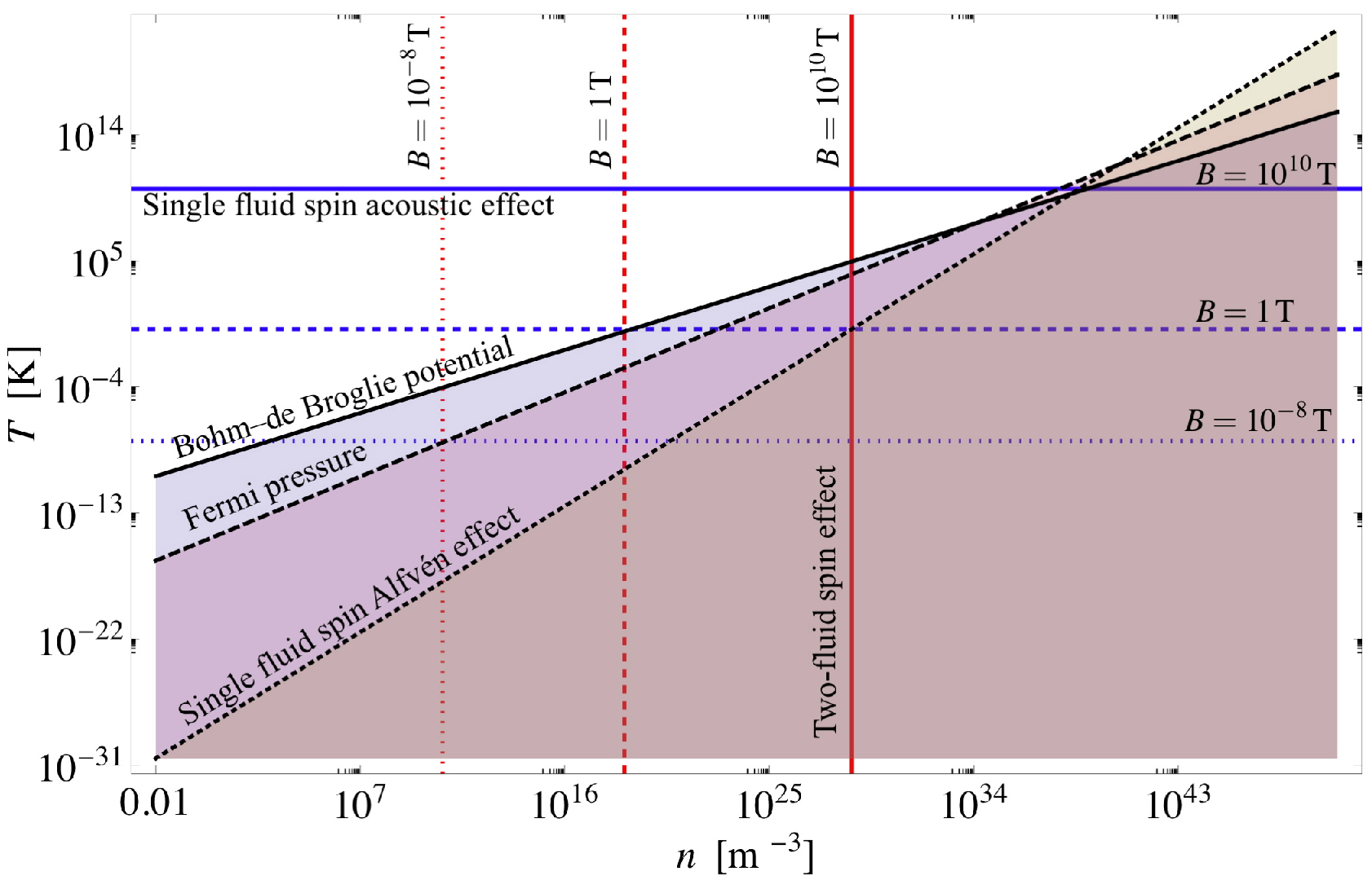
for Alfvén waves propagating parallel to the magnetic field was derived, where $B_{1}$ is the slowly varying magnetic field amplitude, $v_{g}^{\prime}=dv_{g}/dk$ is the group dispersion, $\zeta=z-v_{g}t$ is the comoving coordinate and $v_{g}$ is the group velocity. These quantities are determined from the Alfvén wave dispersion relation, which reads $\omega^{2}=k^{2}c_{A}^{2}(1\pm kc_{A}/\omega_{ci})$, when weakly dispersive effects due to the Hall current is included [61]. Here $c_{A}$ is the Alfvén velocity and $\omega_{ci}$ is the ion-cyclotron frequency. The upper (lower) sign corresponds to right (left) hand circular polarization. The nonlinear coefficient is $Q=Q_{c}[1-({2}$$\mu_{B}B_{0}$$/{m_{i}c_{A}^{2}})^{2}]$, where the classical coefficient is $Q_{c}=kc_{A}^{3}/4(c_{A}^{2}-c_{s}^{2})$ $\simeq-kc_{A}^{3}/4c_{s}^{2}$, where $c_{s}$ is the ion-sound speed. Although linearly the modification of the Alfvén waves can be neglected (for modest temperature and densities), the nonlinear coefficient $Q$ could be significantly affected by the spin terms. Illustration of the parameters needed to make the different quantum plasma effects significant, is shown in Fig. 1. In particular we note that the two-fluid nonlinear spin effects are important for high plasma densities and/or a weak (external) magnetic fields. For comparison, both the Fermi pressure and the Bohm–de Broglie potential need a low-temperature or a very high density to be significant.. A somewhat surprising result is that here nonlinear spin effects tend to be more important for a lower magnetic field, whereas the opposite is true for linear spin effects.

As a second example of spin fluid effects we will consider the ponderomotive force of an electromagnetic wave propagating along an external magnetic field . Classically, the density fluctuations induced by the ponderomotive force of an electromagnetic (EM) wave lead to an electrostatic wake field [62], as used in advanced particle accelerator schemes [63]. In other regimes, the back-reaction on the EM-wave due to the density fluctuations leads to phenomena such as soliton formation, self-focusing or wave collapse [64, 65]. When spin effects based on Eqs. (25)-(26) are included, the spin-contribution to the ponderomotive force, resulting from the combined effect of the magnetic dipole force and spin-precession, leads to a separation of spin-up and -down populations. The expression for the ponderomotive force density for electromagnetic waves propagating along the unperturbed magnetic field $\mathbf{B}_{0}=B_{0}\mathbf{z}$ can be divided into its classical part

$$F_{\mathrm{c}z}=-\frac{e^{2}}{2m^{2}\omega\left(\omega\pm\omega_{c}\right)}\left[\frac{\partial}{\partial z}\pm\frac{k\omega_{c}}{\omega\left(\omega\pm\omega_{c}\right)}\frac{\partial}{\partial t}\right]|E|^{2}.$$

(75)

where $+(-)$ correspond to right (left) hand circular polarization, and the spin part

$$F_{\alpha z}=\mp\frac{2\mu^{2}}{m\hbar}\frac{S_{0\alpha}}{\left(\omega\pm\omega_{g}\right)}\left[\frac{\partial}{\partial z}-\frac{k}{\left(\omega\pm\omega_{g}\right)}\frac{\partial}{\partial t}\right]|B|^{2}.$$

(76)

[68]. Here $E$ and $B$ are the electric and magnetic field amplitude, respectively, $\omega_{c}=eB_{0}/m$ is the cyclotron frequency, $\omega_{g}=2\mu B_{0}/\hbar=g\omega_{c}/2$. The index $\alpha=(u,d)$ refers to the up- and down populations, respectively. In particular the up- and down spin vector components are $S_{0u}=1$, and $S_{0d}=-1$. Thus it is clear that the spin-part of the ponderomotive force induces a separation of the up- and down-populations. This effect survives also in the absence of an external magnetic field, and it turns out that the magnitude of the relative up-and down density perturbations can be larger than the classical density perturbations in an unmagnetized plasma, provided

$$1<\frac{\hbar\omega}{mc^{2}}\frac{\omega_{p}^{2}L^{2}}{c^{2}}$$

(77)

where $L$ is the pulse length of the high-frequency pulse. The first factor of the right hand side of (77) is smaller than unity for frequencies below the Compton frequency, but the second factor can be large for long pulse lengths, and hence large spin-polarization can be induced by a sufficiently long EM-pulse in an unmagnetized plasma for optical frequencies and higher. Once the plasma is spin-polarized, the spin terms in the evolution equations can be important for the dynamics. For further studies of results from spin-fluid theories, see e.g. Refs. [66, 67].

References

- [1] P. K. Shukla and B. Eliasson, Phys. Usp. 53, 51 (2010).
- [2] P. R. Holland, The Quantum Theory of Motion (Cambridge University Press, Cambridge, 1993).
- [3] J. Dawson, Phys. Fluids 4, 869 (1961).
- [4] D. Pines, J. Nucl. Energy C: Plasma Phys. 2, 5 (1961).
- [5] F. Haas, G. Manfredi, and M. R. Feix, Phys. Rev. E 62, 2763 (2000).
- [6] D. Anderson, B. Hall, M. Lisak, and M. Marklund, Phys. Rev. E 65, 046417 (2002).
- [7] E. Wigner, Phys. Rev. 40, 749 (1932).
- [8] J. E. Moyal, Proc. Cambridge Philos. Soc. 45, 99 (1949).
- [9] J. T. Mendonca, Theory of Photon Acceleration (IOP Publishing, 2001).
- [10] W. P. Schleich, Quantum Optics in Phase Space (Wiley, 2001).
- [11] M. Marklund, Phys. Plasmas 12, 082110 (2005).
- [12] G. Manfredi, Fields Inst. Comm. 46, 263 (2005).
- [13] M. Marklund and G. Brodin, Phys. Rev. Lett. 98, 025001 (2007).
- [14] G. Brodin and M. Marklund, New J. Phys. 9, 277 (2007).
- [15] S. R. de Groot and L. G. Suttorp, Foundations of Electrodynamics (North-Holland, 1972).
- [16] H. Alfvén, Nature 150, 405 (1942).
- [17] B. I. Halperin and P. C. Hohenberg, Phys. Rev. 188, 898 (1969).
- [18] A. V. Balatsky, Phys. Rev. B 42, 8103 (1990).
- [19] U. W. Rathe, C. H. Keitel, M. Protopapas, and P. L. Knight, J. Phys. B: At. Mol. Opt. Phys. 30, L531 (1997).
- [20] S. X. Hu and C. H. Keitel, Phys. Rev. Lett. 83, 4709 (1999).
- [21] R. Arvieu, P. Rozmej, and M. Turek, Phys. Rev. A 62, 022514 (2000).
- [22] J. R. Vázquez de Aldana and L. Roso, J. Phys. B: At. Mol. Opt. Phys. 33, 3701 (2000).
- [23] M. W. Walser and C. H. Keitel, J. Phys. B: At. Mol. Opt. Phys. 33, L221 (2000).
- [24] Z. Qian and G. Vignale, Phys. Rev. Lett. 88, 056404 (2002).
- [25] M. W. Walser, D. J. Urbach, K. Z. Hatsagortsyan, S. X. Hu, and C. H. Keitel, Phys. Rev. A 65, 043410 (2002).
- [26] J. S. Roman, L. Roso, and L. Plaja, J. Phys. B: At. Mol. Opt. Phys. 37, 435 (2004).
- [27] R. L. Liboff, Europhys. Lett. 68, 577 (2004).
- [28] J. N. Fuchs, D. M. Gangardt, T. Keilman, and G. V. Shlyapnikov, Phys. Rev. Lett. 95, 150402 (2005).
- [29] K. Kirsebom et al., Phys. Rev. Lett. 87, 054801 (2001).
- [30] H. Weyl, The Theory of Groups and Quantum Mechanics (Dover, New York, 1931).
- [31] R. J. Glauber, Phys. Rev. 131, 2766 (1963).
- [32] U. Leonhardt, Measuring the Quantum State of Light, (Cambridge University Press, Cambridge 1997).
- [33] H. W. Lee, and M. OṠcully, Found. Phys. 13, 61 (1983).
- [34] P. Carruthers, and F. Zachariasen, Rev. Mod. Phys. 55, 245 (1983).
- [35] K. Takahashi, Prog. Theor. Phys. Supp. 98, 109 (1989).
- [36] H. Haug, and A-P Jauho Quantum Kinetics in Transport and Optics of Semiconductors (Springer Series in Solid-State Sciences vol 123) (Berlin: Springer 2007).
- [37] J. Rammer, Quantum Transport Theory (Cambridge: Cambridge University Press 2007).
- [38] R. J. Glauber, Phys. Rev. 130, 2529 (1963).
- [39] E. C. G. Sudarshan, Phys. Rev. Lett. 10, 277 (1963).
- [40] R. J. Glauber, Quantum Optics and Electronics edited by C. Dewitt, A. Blandin and C. Cohen-Tannoudji (Gordon and Breach, New York, 1965).
- [41] K. Husimi, Prog. Phys. Math. Soc. Japan 22, 264 (1940).
- [42] H. W. Lee, Phys. Rep. 259, 147 (1995).
- [43] R. L. Stratonovich, Sov. Phys. D 1, 414 (1956).
- [44] O. Serimaa, J. Javanainen, and S. Varro, Phys. Rev. A 33, 2913 (1986).
- [45] L. Cohen, and M. Scully, Found. Phys. 16, 295 (1986).
- [46] C. Chandler, L. Cohen, C. Lee, and M. Scully, Found. Phys. 22, 267 (1992).
- [47] M. Scully, and K. Wodkiewicz, Found. Phys. 24, 85 (1994).
- [48] M. Cunha, V. Man’ko, and M. Scully, Found. Phys. Lett. 14, 103 (2001).
- [49] J. Zamanian, M. Marklund, and G. Brodin, New J. Phys. 12, 043019 (2010).
- [50] J. Schwinger, Phys. Rev. 73, 416 (1948).
- [51] G. Brodin, M. Marklund, J. Zamanian, A. Ericsson, and L. P. Mana, Phys. Rev. Lett. 101, 245002 (2008).
- [52] S. C. Cowley, R. M. Kulsrud, and E. Valeo, Phys. Fluids 29, 430 (1986).
- [53] D. Nicholson, Introduction to Plasma Theory, (John Wiley & Sons Inc 1983).
- [54] F. Haas, Phys. Plasmas 12, 062117 (2005).
- [55] F. Haas, M. Marklund, G. Brodin, and J. Zamanian, Phys. Lett. A 374, 481 (2010).
- [56] F. Haas, J. Zamanian, M. Marklund, and G. Brodin, New. J. Phys. 12, 073027 (2010).
- [57] J. Zamanian, M. Stefan, M. Marklund, and G. Brodin, Phys. Plasma, in press (2010).
- [58] W. Zhang, and R. Balescu, J. Plasma Phys. 40, 199 (1988).
- [59] R. Balescu, and W. Zhang, J. Plasma Phys. 40, 215 (1988).
- [60] G. Brodin, M. Marklund and G. Manfredi, Phys. Rev. Lett. 100, 175001 (2008).
- [61] G. Brodin and L. Stenflo, Contrib. Plasma Phys. 30, 413 (1990).
- [62] L. M. Gorbunov and V. I. Kirsanov, Zh. Eksp. Teor. Fiz. 93, 509 (1987) [Sov. J. Plasma Phys. 93, 290 (1987)].
- [63] R. Bingham, Nature 445, 721 (2007).
- [64] L. Berge, Phys. Reports 303 259 (1998)
- [65] P. K. Shukla, N. N. Rao, M. Y. Yu and N. L. Tsintsadze, Phys. Reports, 138, 1 (1986).
- [66] G. Brodin and M. Marklund, Phys. Rev. E 76, 055403 (2007).
- [67] G. Brodin and M. Marklund, Phys. Plasmas 14, 112107 (2007).
- [68] G. Brodin, A. P. Misra, M. Marklund, Phys. Rev. Lett. 105, 105004 (2010)
- [69] P. S. Moya and F. A Asenjo, arXiv 1005.2573 [physics-plasm-ph]
- [70] J. Lundin and G. Brodin, arXiv:1006.1310v1 [physics.plasm-ph]