Regularizers for Structured Sparsity
Charles A. Micchelli(1),(2)
Jean M. Morales(3)
Massimiliano Pontil(3)
(1)
Department of Mathematics
City University of Hong Kong
83 Tat Chee Avenue, Kowloon Tong
Hong Kong
(2) Department of Mathematics and Statistics
State University of New York
The University at Albany
1400 Washington Avenue
Albany, NY, 12222, USA
(3) Department of Computer Science
University College London
Gower Street, London WC1E
England, UK
E-mail: {m.pontil,j.morales}@cs.ucl.ac.uk
We study the problem of learning a sparse linear regression vector under additional conditions on the structure of its sparsity pattern. This problem is relevant in machine learning, statistics and signal processing. It is well known that a linear regression can benefit from knowledge that the underlying regression vector is sparse. The combinatorial problem of selecting the nonzero components of this vector can be “relaxed” by regularizing the squared error with a convex penalty function like the norm. However, in many applications, additional conditions on the structure of the regression vector and its sparsity pattern are available. Incorporating this information into the learning method may lead to a significant decrease of the estimation error.
In this paper, we present a family of convex penalty functions, which encode prior knowledge on the structure of the vector formed by the absolute values of the regression coefficients. This family subsumes the norm and is flexible enough to include different models of sparsity patterns, which are of practical and theoretical importance. We establish the basic properties of these penalty functions and discuss some examples where they can be computed explicitly. Moreover, we present a convergent optimization algorithm for solving regularized least squares with these penalty functions. Numerical simulations highlight the benefit of structured sparsity and the advantage offered by our approach over the Lasso method and other related methods.
1 Introduction
The problem of sparse estimation is becoming increasing important in statistics, machine learning and signal processing. In its simplest form, this problem consists in estimating a regression vector from a set of linear measurements , obtained from the model
| (1.1) |
where is an matrix, which may be fixed or randomly chosen and is a vector which results from the presence of noise.
An important rational for sparse estimation comes from the observation that in many practical applications the number of parameters is much larger than the data size , but the vector is known to be sparse, that is, most of its components are equal to zero. Under this sparsity assumption and certain conditions on the data matrix , it has been shown that regularization with the norm, commonly referred to as the Lasso method [27], provides an effective means to estimate the underlying regression vector, see for example [5, 7, 18, 28] and references therein. Moreover, this method can reliably select the sparsity pattern of [18], hence providing a valuable tool for feature selection.
In this paper, we are interested in sparse estimation under additional conditions on the sparsity pattern of the vector . In other words, not only do we expect this vector to be sparse but also that it is structured sparse, namely certain configurations of its nonzero components are to be preferred to others. This problem arises is several applications, ranging from functional magnetic resonance imaging [9, 29], to scene recognition in vision [10], to multi-task learning [1, 15, 23] and to bioinformatics [26], see [14] for a discussion.
The prior knowledge that we consider in this paper is that the vector , whose components are the absolute value of the corresponding components of , should belong to some prescribed convex subset of the positive orthant. For certain choices of this implies a constraint on the sparsity pattern as well. For example, the set may include vectors with some desired monotonicity constraints, or other constraints on the “shape” of the regression vector. Unfortunately, the constraint that is nonconvex and its implementation is computational challenging. To overcome this difficulty, we propose a family of penalty functions, which are based on an extension of the norm used by the Lasso method and involves the solution of a smooth convex optimization problem. These penalty functions favor regression vectors such that , thereby incorporating the structured sparsity constraints.
Precisely, we propose to estimate as a solution of the convex optimization problem
| (1.2) |
where denotes the Euclidean norm, is a positive parameter and the penalty function takes the form
As we shall see, a key property of the penalty function is that it exceeds the norm of when , and it coincides with the norm otherwise. This observation suggests a heuristic interpretation of the method (1.2): among all vectors which have a fixed value of the norm, the penalty function will encourage those for which . Moreover, when the function reduces to the norm and, so, the solution of problem (1.2) is expected to be sparse. The penalty function therefore will encourage certain desired sparsity patterns. Indeed, the sparsity pattern of is contained in that of the auxiliary vector at the optimum and, so, if the set allows only for certain sparsity patterns of , the same property will be “transferred” to the regression vector .
There has been some recent research interest on structured sparsity, see [11, 13, 14, 19, 22, 30, 31] and references therein. Closest to our approach are penalty methods built around the idea of mixed - norms. In particular, the group Lasso method [31] assumes that the components of the underlying regression vector can be partitioned into prescribed groups, such that the restriction of to a group is equal to zero for most of the groups. This idea has been extended in [14, 32] by considering the possibility that the groups overlap according to certain hierarchical or spatially related structures. Although these methods have proved valuable in applications, they have the limitation that they can only handle more restrictive classes of sparsity, for example patterns forming only a single connected region. Our point of view is different from theirs and provides a means to designing more flexible penalty functions which maintain convexity while modeling richer model structures. For example, we will demonstrate that our family of penalty functions can model sparsity patterns forming multiple connected regions of coefficients.
The paper is organized in the following manner. In Section 2 we establish some important properties of the penalty function. In Section 3 we address the case in which the set is a box. In Section 4 we derive the form of the penalty function corresponding to the wedge with decreasing coordinates and in Section 5 we extends this analysis to the case in which the constraint set is constructed from a directed graph. In Section 6 we discuss useful duality relations and in Section 7 we address the issue of solving the problem (1.2) numerically by means of an alternating minimization algorithm. Finally, in Section 8 we provide numerical simulations with this method, showing the advantage offered by our approach.
A preliminary version of this paper appeared in the proceedings of the Twenty-Fourth Annual Conference on Neural Information Processing Systems (NIPS 2010) [21]. The new version contains Propositions 2.4, 2.3 and 2.4, the description of the graph penalty in Section 5, Section 6, a complete proof of Theorem 7.1 and an experimental comparison with the method of [11].
2 Penalty function
In this section, we provide some general comments on the penalty function which we study in this paper.
We first review our notation. We denote with and the nonnegative and positive real line, respectively. For every we define to be the vector formed by the absolute values of the components of , that is, , where is the set of positive integers up to and including . Finally, we define the norm of vector as and the norm as .
Given an input data matrix and an output vector , obtained from the linear regression model discussed earlier, we consider the convex optimization problem
| (2.1) |
where is a positive parameter, is a prescribed convex subset of the positive orthant and the function is given by the formula
Note that in (2.1), for a fixed , the infimum over in general is not attained, however, for a fixed , the infimum over is always attained.
Since the auxiliary vector appears only in the second term of the objective function of problem (2.1), and our goal is to estimate , we may also directly consider the regularization problem
| (2.2) |
where the penalty function takes the form
| (2.3) |
Note that is convex on its domain because each of its summands are likewise convex functions. Hence, when the set is convex it follows that is a convex function and (2.2) is a convex optimization problem.
An essential idea behind our construction of the penalty function is that, for every , the quadratic function provides a smooth approximation to from above, which is exact at . We indicate this graphically in Figure 1-a. This fact follows immediately by the arithmetic-geometric mean inequality, which states, for every that .
 |
 |
| (a) | (b) |
A special case of the formulation (2.2) with is the Lasso method [27], which is defined to be a solution of the optimization problem
Indeed, using again the arithmetic-geometric mean inequality it follows that . Moreover, if for every , then the infimum is attained for . This important special case motivated us to consider the general method described above. The utility of (2.3) is that upon inserting it into (2.2) there results an optimization problem over and with a continuously differentiable objective function. Hence, we have succeeded in expressing a nondifferentiable convex objective function by one which is continuously differentiable on its domain.
Our first observation concerns the differentiability of . In this regard, we provide a sufficient condition which ensures this property of , which, although seemingly cumbersome covers important special cases. To present our result, for any real numbers , we define the parallelepiped .
Definition 2.1.
We say that the set is admissible if it is convex and, for all with , the set is a nonempty, compact subset of the interior of .
Proposition 2.1.
If and is an admissible subset of , then the infimum above is uniquely achieved at a point and the mapping is continuous. Moreover, the function is continuously differentiable and its partial derivatives are given, for any , by the formula
| (2.4) |
We postpone the proof of this proposition to the appendix. We note that, since is continuous, we may compute it at a vector , some of whose components are zero, as a limiting process. Moreover, at such a vector the function is in general not differentiable, for example consider the case .
The next proposition provides a justification of the penalty function as a means to incorporate structured sparsity and establish circumstances for which the penalty function is a norm. To state our result, we denote by the closure of the set .
Proposition 2.2.
For every , we have that and the equality holds if and only if . Moreover, if is a nonempty convex cone then the function is a norm and we have that , where and is the canonical basis of .
Proof.
By the arithmetic-geometric mean inequality we have that , proving the first assertion. If , there exists a sequence in , such that . Since it readily follows that . Conversely, if , then there is a sequence in , such that . This inequality implies that some subsequence of this sequence converges to a . Using arithmetic-geometric mean inequality we conclude that and the result follows. To prove the second part, observe that if is a nonempty convex cone, namely, for any and it holds that , we have that is positive homogeneous. Indeed, making the change of variable we see that . Moreover, the above inequality, , implies that if then . The proof of the triangle inequality follows from the homogeneity and convexity of , namely .
Finally, note that if and only if . Since is convex the maximum above is achieved at an extreme point of the unit ball. ∎
This proposition indicates a heuristic interpretation of the method (2.2): among all vectors which have a fixed value of the norm, the penalty function will encourage those for which . Moreover, when the function reduces to the norm and, so, the solution of problem (2.2) is expected to be sparse. The penalty function therefore will encourage certain desired sparsity patterns.
The last point can be better understood by looking at problem (2.1). For every solution , the sparsity pattern of is contained in the sparsity pattern of , that is, the indices associated with nonzero components of are a subset of those of . Indeed, if it must hold that as well, since the objective would diverge otherwise (because of the ratio ). Therefore, if the set favors certain sparse solutions of , the same sparsity pattern will be reflected on . Moreover, the term appearing in the expression for favors sparse vectors. For example, a constraint of the form favors consecutive zeros at the end of and nonzeros everywhere else. This will lead to zeros at the terminal components of as well. Thus, in many cases like this, it is easy to incorporate a convex constraint on , whereas it may not be possible to do the same with .
Next, we note that a normalized version of the group Lasso penalty [31] is included in our setting as a special case. If, for some , forms a partition of the index set , the corresponding group Lasso penalty is defined as
| (2.5) |
where, for every , we use the notation . It is an easy matter to verify that for .
The next proposition presents a useful construction which may be employed to generate new penalty functions from available ones. It is obtained by composing a set with a linear transformation, modeling the sum of the components of a vector, across the elements of a prescribed partition of . To describe our result we introduce the group average map induced by . It is defined, for each , as .
Proposition 2.3.
If , and is a partition of then
Proof.
The idea of the proof depends on two basic observations. The first uses the set theoretic formula
From this decomposition we obtain that
| (2.6) |
Next, we write and decompose the inner infimum as the sum
Now, the second essential step in the proof evaluates the infimum in the second sum by the Cauchy-Schwarz inequality to obtain that
We now substitute this formula into the right hand side of equation (2.6) to finish the proof.∎
When the set is a nonempty convex cone, to emphasize that the function is a norm we denoted it by . We end this section with the identification of the dual norm of , which is defined as
Proposition 2.4.
If is a nonempty convex cone then there holds the equation
Proof.
By definition, is the smallest constant such that, for every and , it holds that
Minimizing the left hand side of this inequality for yields the equivalent inequality
Since this inequality holds for every , the result follows by taking the supremum of the right hand side of the above inequality over this set. ∎
The formula for the dual norm suggests that we introduce the set . With this notation we see that the dual norm becomes
Moreover, a direct computation yields an alternate form for the original norm given by the equation
3 Box penalty
We proceed to discuss some examples of the set which may be used in the design of the penalty function .
The first example, which is presented in this section, corresponds to the prior knowledge that the magnitude of the components of the regression vector should be in some prescribed intervals. We choose , , and define the corresponding box as The theorem below establishes the form of the box penalty. To state our result, we define, for every , the function .
Theorem 3.1.
We have that
Moreover, the components of the vector are given by the equations , .
Proof.
Since it suffices to establish the result in the case . We shall show that if , then
| (3.1) |
Since both sides of the above equation are continuous functions of it suffices to prove this equation for . In this case, the function is strictly convex, and so, has a unique minimum in at , see also Figure 1-b. Moreover, if the minimum occurs at , whereas if , it occurs at . This establishes the formula for . Consequently, we have that
Equation (3.1) now follows by a direct computation. ∎
4 Wedge penalty
In this section, we consider the case that the coordinates of the vector are ordered in a nonincreasing fashion. As we shall see, the corresponding penalty function favors regression vectors which are likewise nonincreasing.
We define the wedge
Our next result describes the form of the penalty in this case. To explain this result we require some preparation. We say that a partition of is contiguous if for all , , it holds that . For example, if , partitions and are contiguous but is not.
Definition 4.1.
Given any two disjoint subsets we define the region in
| (4.1) |
Note that the boundary of this region is determined by the zero set of a homogeneous polynomial of degree two. We also need the following construction.
Definition 4.2.
For every we set and label the elements of in increasing order as . We associate with the set a contiguous partition of , given by , where we define , and set and .
Figure 2 illustrates an example of a contiguous partition along with the set .

A subset of also induces two regions in which play a central role in the identification of the wedge penalty. First, we describe the region which “crosses over” the induced partition . This is defined to be the set
| (4.2) |
In other words, if the average of the square of its components within each region strictly decreases with . The next region which is essential in our analysis is the “stays within” region, induced by the partition . This region is defined as
| (4.3) |
where denotes the closure of the set and we use the notation . In other words, all vectors within this region have the property that, for every set , the average of the square of a first segment of components of within this set is not greater than the average over . We note that if is the empty set the above notation should be interpreted as and
From the cross-over and stay-within sets we define the region
Alternatively, we shall describe below the set in terms of two vectors induced by a vector and the set . These vectors play the role of the Lagrange multiplier and the minimizer for the wedge penalty in the theorem below.
Definition 4.3.
For every vector and every subset we let be the induced contiguous partition of and define two vectors and by
and
| (4.4) |
Note that the components of are constant on each set , .
Lemma 4.1.
For every and we have that
- (a)
if and only if and ;
- (b)
If and then .
Proof.
The first assertion follows directly from the definition of the requisite quantities. The proof of the second assertion is a direct consequence of the fact that the vector is a constant on any element of the partition and strictly decreasing from one element to the next in that partition. ∎
For the theorem below we introduce, for every the sets
We shall establishes not only that the collection of sets form a partition of , that is, their union is and two distinct elements of are disjoint, but also explicitly determine the wedge penalty on each element of .
Theorem 4.1.
The collection of sets form a partition of . For each there is a unique such that , and
| (4.5) |
where . Moreover, the components of the vector are given by the equations , where
| (4.6) |
Proof.
First, let us observe that there are inequality constraints defining . It readily follows that all vectors in this constraint set are regular, in the sense of optimization theory, see [4, p. 279]. Hence, we can appeal to [4, Prop. 3.3.4, p. 316 and Prop. 3.3.6, p. 322], which state that is a solution to the minimum problem determined by the wedge penalty, if and only if there exists a vector with nonnegative components such that
| (4.7) |
where we set Furthermore, the following complementary slackness conditions hold true
| (4.8) |
To unravel these equations, we let , which is the subset of indexes corresponding to the constraints that are not tight. When , we express this set in the form where . As explained in Definition 4.2, the set induces the partition of . When our notation should be interpreted to mean that is empty and the partition consists only of . In this case, it is easy to solve equations (4.7) and (4.8). In fact, all components of the vector have a common value, say , and by summing both sides of equation (4.7) over we obtain that
Moreover, summing both sides of the same equation over we obtain that
and, since we conclude that .
We now consider the case that . Hence, the vector has equal components on each subset , which we denote by , . The definition of the set implies that the sequence is strictly decreasing and equation (4.8) implies that , for every . Summing both sides of equation (4.7) over we obtain that
| (4.9) |
from which equation (4.6) follows. Since the are strictly decreasing, we conclude that . Moreover, choosing and summing both sides of equations (4.7) over we obtain that
which implies that . Since this holds for every and we conclude that and therefore, it follows that .
In summary, we have shown that , , and . In particular, this implies that the collection of sets covers . Next, we show that the elements of are disjoint. To this end, we observe that, the computation described above can be reversed. That is to say, conversely for any and we conclude that and solve the equations (4.7) and (4.8). Since the wedge penalty function is strictly convex we know that equations (4.7) and (4.8) have a unique solution. Now, if then it must follow that . Consequently, by part (b) in Lemma 4.1 we conclude that . ∎
Note that the set and the associated partition appearing in the theorem is identified by examining the optimality conditions of the optimization problem (2.3) for . There are possible partitions. Thus, for a given , determining the corresponding partition is a challenging problem. We explain how to do this in Section 7.
An interesting property of the Wedge penalty, which is indicated by Theorem 4.1, is that it has the form of a group Lasso penalty as in equation (2.5), with groups not fixed a-priori but depending on the location of the vector . The groups are the elements of the partition and are identified by certain convex constraints on the vector . For example, for we obtain that if and otherwise. For , we have that
 |
 |
 |
 |
 |
| (a) | (b) | (c) | (d) | (e) |
where we have also displayed the partition involved in each case. We also present a graphical representation of the corresponding unit ball in Figure 3-a. For comparison we also graphically display the unit ball for the hierarchical group Lasso with groups and two group Lasso in Figure 3-b,c,d, respectively.
The wedge may equivalently be expressed as the constraint that the difference vector is less than or equal to zero. This alternative interpretation suggests the -th order difference operator, which is given by the formula
and the corresponding -th wedge
| (4.10) |
The associated penalty encourages vectors whose sparsity pattern is concentrated on at most different contiguous regions. Note that is not the wedge considered earlier. Moreover, the -wedge includes vectors which have a convex “profile” and whose sparsity pattern is concentrated either on the first elements of the vector, on the last, or on both.
5 Graph penalty
In this section we present an extension of the wedge set which is inspired by previous work on the group Lasso estimator with hierarchically overlapping groups [32]. It models vectors whose magnitude is ordered according to a graphical structure.
Let be a directed graph, where is the set of vertices in the graph and is the edge set, whose cardinality is denoted by . If we say that there is a directed edge from vertex to vertex . The graph is identified by the incidence matrix, which we define as
We consider the penalty for the convex cone and assume, from now on, that is acyclic (DAG), that is, has no directed loops. In particular, this implies that, if then . The wedge penalty described above is a special case of the graph penalty corresponding to a line graph. Let us now discuss some aspects of the graph penalty for an arbitrary DAG. As we shall see, our remarks lead to an explicit form of the graph penalty when is a tree.
If we say that vertex is a child of vertex and is a parent of . For every vertex , we let and be the set of children and parents of , respectively. When is a tree, is the empty set if is the root node and otherwise consists of only one element, the parent of , which we denote by .
Let be the set of descendants of , that is, the set of vertices which are connected to by a directed path starting in , and let be the set of ancestors of , that is, the set of vertices from which a directed path leads to . We use the convention that and .
Every connected subset induces a subgraph of which is also a DAG. If and are disjoint connected subsets of , we say that they are connected if there is at least one edge connecting a pair of vertices in and , in either one or the other direction. Moreover, we say that is below — written — if and are connected and every edge connecting them departs from a node of .
Definition 5.1.
Let be a DAG. We say that is a cut of if it induces a partition of the vertex set such that if and only if vertices and belong to two different elements of the partition.
In other words, a cut separates a connected graph in two or more connected components such that every pair of vertices corresponding to a disconnected edge, that is an element of , are in two different components. We also denote by the set of cuts of , and by the set of descendants of within set , for every and .
Next, for every , we define the regions in by the equations
| (5.1) |
and
| (5.2) |
These sets are the graph equivalent of the sets defined by equations (4.2) and (4.3) in the special case of the wedge penalty in Section 4. We also set .
Moreover, for every , we define the sets
As of yet, we cannot extend Theorem 4.1 to the case of an arbitrary DAG. However, we can accomplish this when is a tree.
Lemma 5.1.
Let be a tree, let be the associated incidence matrix and let . The following facts are equivalent:
- (a)
For every it holds that
- (b)
The linear system admits a non-negative solution for .
Proof.
The incident matrix of a tree has the property that, for every and ,
| (5.3) |
where, for every , if and zero otherwise. The linear system in (b) can be written componentwise as
Summing both sides of this equation over and using equation (5.3), we obtain the equivalent equations
The result follows. ∎
Definition 5.2.
Let be a DAG. For every vector and every cut we let , be the partition of induced by , and define two vectors and . The components of are given as
whereas the components of are given by
| (5.4) |
Note that the notation we adopt in this definition differs from that used in the case of line graph, given in Definition 4.3. However, Definition 5.2 leads to a more appropriate presentation of our results for a tree.
Proposition 5.1.
Let be a tree and the associated incidence matrix. For every and every cut we have that
- (a)
if and only if , and , for all , , ;
- (b)
If and then .
Proof.
We immediately see that if and only if and for all , , . Moreover, by applying Lemma 5.1 on each element of the partition induced by and choosing , we conclude that if and only if . This proves the first assertion.
The proof of the second assertion is a direct consequence of the fact that the vector is a constant on any element of the partition and strictly decreasing from one element to the next in that partition. ∎
Theorem 5.1.
Let be a tree. The collection of sets form a partition of . Moreover, for every there is a unique such that
| (5.5) |
and the vector has components given by , , where
| (5.6) |
Proof.
The proof of this theorem proceeds in a fashion similar to that of Theorem 4.1. In this regard, Lemma 5.1 is crucial. By KKT theory (see e.g. [4, Theorems 3.3.4,3.3.7]), is an optimal solution of the graph penalty if and only if there exists such that, for every
and the following complementary conditions hold true
| (5.7) |
We rewrite the first equation as
| (5.8) |
Now, if solves equations (5.7) and (5.8), then it induces a cut and a corresponding partition of such that for every . That is, for every , , and for every . Therefore, summing equations (5.8) for we get that
Moreover, since , if we see that . Next, for every and we sum both sides of equation (5.8) for to obtain that
| (5.9) |
We see that and conclude that .
In summary we have shown that the collection of sets cover . Next, we show that the elements of are disjoint. To this end, we observe that, the computation described above can be reversed. That is to say, conversely for any partition of and we conclude by Proposition 5.1 that the vectors and solves the KKT optimality conditions. Since this solution is unique if then it must follow that , which implies that . ∎
Theorems 4.1 and 5.1 fall into the category of a set chosen in the form of a polyhedral cone, that is
where is an matrix. Furthermore, in the line graph of Theorem 4.1 and also the extension in Theorem 5.1 the matrix only has elements which are or . These two examples that we considered led to explicit description of the norm . However, there are seemingly simple cases of a matrix of this type where the explicit computation of the norm seem formidable, if not impossible. For example, if , and
we are led by KKT to a system of equations that, in the case of two active constraints, that is, , are the common zeros of two fourth order polynomials in the vector .
6 Duality
In this section, we comment on the utility of the class of penalty functions considered in this paper, which is fundamentally based on their construction as constrained infimum of quadratic functions. To emphasize this point both theoretically and computationally, we discuss the conversion of the regularization variational problem over , namely
| (6.1) |
where
into a variational problem over .
To explain what we have in mind, we introduce the following definition.
Definition 6.1.
For every , we define the vector as
where .
Note that .
Theorem 6.1.
For , , any matrix and any nonempty convex set we have that
| (6.2) |
Moreover, if is a solution to this problem, then is a solution to problem (6.1).
Proof.
We substitute the formula for into the right hand side of equation (6.1) to obtain that
| (6.3) |
where we define
A straightforward computation yields that
Since , we conclude that any minimizing sequence for the optimization problem on the right hand side of equation (6.3) must have a subsequence which converges. These remarks confirm equation (6.2).
We now prove the second claim. For a direct computation confirms that
Note that the right hand side of this equation provides a continuous extension of the left hand side to . For notational simplicity, we still use the left hand side to denote this continuous extension.
By a limiting argument, we conclude, for every , that
| (6.4) |
We are now ready to complete the proof of the theorem. Let be a solution for the optimization problem (6.2). By definition, it holds, for any and , that
Combining this inequality with inequality (6.4) evaluated at , we conclude that
from which the result follows. ∎
An important consequence of the above theorem is a method to find a solution to the optimization problem (6.1) from a solution to the optimization problem (6.2). We illustrate this idea in the case that .
Corollary 6.1.
It holds that
| (6.5) |
Moreover, if is a solution of the right optimization problem then the vector , whose components are defined for as
| (6.6) |
is a solution of the left optimization problem problem.
We further discuss two choices of the set in which we are able to solve problem (6.5) analytically. The first case we consider is , which corresponds to the Lasso penalty. It is an easy matter to see that and the corresponding regression vector is obtained by the well-known “soft thresolding” formula . The second case is the Wedge penalty. We find that the solution of the optimization problem in the right hand side of equation (6.5) is , where is given in Theorem 4.1. Finally, we note that Corollary 6.1 and the example following it extend to the case that by replacing throughout the vector by the vector . In the statistical literature this setting is referred to as orthogonal design.
7 Optimization method
In this section, we address the issue of implementing the learning method (2.2) numerically.
Since the penalty function is constructed as the infimum of a family of quadratic regularizers, the optimization problem (2.2) reduces to a simultaneous minimization over the vectors and . For a fixed , the minimum over is a standard Tikhonov regularization and can be solved directly in terms of a matrix inversion. For a fixed , the minimization over requires computing the penalty function (2.3). These observations naturally suggests an alternating minimization algorithm, which has already been considered in special cases in [1]. To describe our algorithm we choose and introduce the mapping , whose -th coordinate at is given by
For , we also let .
The alternating minimization algorithm is defined as follows: choose and, for , define the iterates
| (7.1) | |||||
| (7.2) |
The following theorem establishes convergence of this algorithm.
Theorem 7.1.
Proof.
We divide the proof into several steps. To this end, we define
and note that .
Step 1. We define two sequences, and and observe, for any , that
| (7.3) |
These inequalities follow directly from the definition of the alternating algorithm, see equations (7.1) and (7.2).
Step 2. We define the compact set . From the first inequality in Proposition 2.2 and inequality (7.3) we conclude, for every , that .
Step 3. We define the function at as
We claim that is continuous on . In fact, there exists a constant such that, for every , it holds that
| (7.4) |
The essential ingredient in the proof of this inequality is the fact that there exists constant and such that, for all , . This follows from the inequalities developed in the proof of Proposition 2.4.
Step 4. By step 2, there exists a subsequence which converges to and, for all and , it holds that
| (7.5) |
Indeed, from step 1 we conclude that there exists such that
Since, by Proposition 2.4 is continuous for , we obtain that
By the definition of the alternating algorithm, we have, for all and , that
From this inequality we obtain, passing to limit, inequalities (7.5).
Step 5. The vector is a stationary point. Indeed, since is admissible, by step 3, . Therefore, since is continuously differentiable this claim follows from step 4.
Step 6. The alternating algorithm converges. This claim follows from the fact that is strictly convex. Hence, has a unique global minimum in , which in virtue of inequalities (7.5) is attained at .
The last claim in the theorem follows from the fact that the set is bounded and the function is continuous. ∎
The most challenging step in the alternating algorithm is the computation of the vector . Fortunately, if is a second order cone, problem (2.3) defining the penalty function may be reformulated as a second order cone program (SOCP), see e.g. [6]. To see this, we introduce an additional variable and note that
In particular, the examples discussed in Sections 4 and 5, the set is formed by linear constraints and, so, problem (2.3) is an SOCP. We may then use available tool-boxes to compute the solution of this problem. However, in special cases the computation of the penalty function may be significantly facilitated by using available analytical formulas. Here, for simplicity we describe how to do this in the case of the wedge penalty. For this purpose we say that a vector is admissible if, for every , it holds that .
The proof of the next lemma is straightforward and we do not elaborate on the details.
Lemma 7.1.
If and are admissible and then is admissible.
| Initialization: |
| Input: ; Output: |
| for to do |
| ; |
| while and |
| end |
| end |
The iterative algorithm presented in Figure 4 can be used to find the partition and, so, the vector described in Theorem 4.1. The algorithm processes the components of vector in a sequential manner. Initially, the first component forms the only set in the partition. After the generic iteration , where the partition is composed of sets, the index of the next components, , is put in a new set . Two cases can occur: the means of the squares of the sets are in strict descending order, or this order is violated by the last set. The latter is the only case that requires further action, so the algorithm merges the last two sets and repeats until the sets in the partition are fully ordered. Note that, since the only operation performed by the algorithm is the merge of admissible sets, Lemma 7.1 ensures that after each step the current partition satisfies the “stay within” conditions , for every and every subset formed by the first elements of . Moreover, the while loop ensures that after each step the current partition satisfies, for every , the “cross over” conditions . Thus, the output of the algorithm is the partition defined in Theorem 4.1. In the actual implementation of the algorithm, the means of squares of each set can be saved. This allows us to compute the mean of squares of a merged set as a weighted mean, which is a constant time operation. Since there are consecutive terms in total, this is also the maximum number of merges that the algorithm can perform. Each merge requires exactly one additional test, so we can conclude that the running time of the algorithm is linear.
8 Numerical simulations
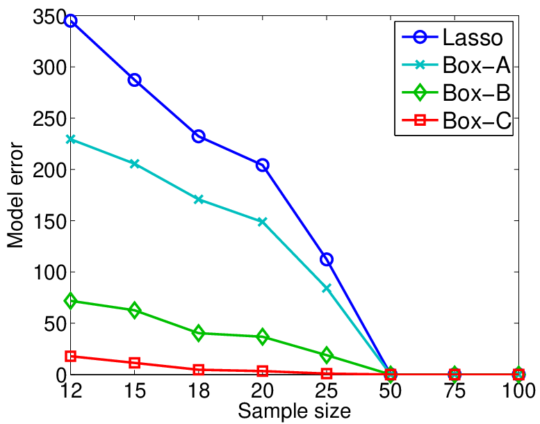
In this section we present some numerical simulations with the proposed method. For simplicity, we consider data generated noiselessly from , where is the true underlying regression vector, and is an input matrix, being the sample size. The elements of are generated i.i.d. from the standard normal distribution, and the columns of are then normalized such that their norm is . Since we consider the noiseless case, we solve the interpolation problem , for different choices of the penalty function . In practice, (2.2) is solved for a tiny value of the parameter, for example, , which we found to be sufficient to ensure that the error term in (2.2) is negligible at the minimum. All experiments were repeated times, generating each time a new matrix . In the figures we report the average of the model error of the vector learned by each method, as a function of the sample size . The former is defined as . In the following, we discuss a series of experiments, corresponding to different choices for the model vector and its sparsity pattern. In all experiments, we solved the optimization problem (2.2) with the algorithm presented in Section 7. Whenever possible we solved step (7.2) using analytical formulas and resorted to the solver CVX (http://cvxr.com/cvx/) in the other cases. For example, in the case of the wedge penalty, we found that the computational time of the algorithm in Figure 4 is faster than that of the solver CVX for , respectively. Our implementation ran on a 16GM memory dual core Intel machine. The MATLAB code is available at http://www.cs.ucl.ac.uk/staff/M.Pontil/software.html.
 |
 |
| (a) | (b) |
 |
 |
| (c) | (d) |
Box. In the first experiment the model is -sparse, where each nonzero component, in a random position, is an integer uniformly sampled in the interval . We wish to show that the more accurate the prior information about the model is, the more precise the estimate will be. We use a box penalty (see Theorem 3.1) constructed “around” the model, imagining that an oracle tells us that each component is bounded within an interval. We consider three boxes of different sizes, namely and and radii and , which we denote as Box-A, Box-B and Box-C, respectively. We compare these methods with the Lasso – see Figure 5-a. As expected, the three box penalties perform better. Moreover, as the radius of a box diminishes, the amount of information about the true model increases, and the performance improves.
Wedge. In the second experiment, we consider a regression vector, whose components are nonincreasing in absolute value and only a few are nonzero. Specifically, we choose a -sparse vector: , if and zero otherwise. We compare the Lasso, which makes no use of such ordering information, with the wedge penalty (see Theorem 4.1) and the hierarchical group Lasso in [32], which both make use of such information. For the group Lasso we choose , with , . These two methods are referred to as “Wedge” and “GL-lin” in Figure 5-b, respectively. As expected both methods improve over the Lasso, with “GL-lin” being the best of the two. We further tested the robustness of the methods, by adding two additional nonzero components with value of to the vector in a random position between and . This result, reported in Figure 5-c, indicates that “GL-lin” is more sensitive to such a perturbation.
Composite wedge. Next we consider a more complex experiment, where the regression vector is sparse within different contiguous regions , and the norm on one region is larger than the norm on the next region. We choose sets , and generate a -sparse vector whose -th nonzero element has value (decreasing) and is in a random position in , for . We encode this prior knowledge by choosing with . This method constraints the sum of the sets to be nonincreasing and may be interpreted as the composition of the wedge set with an average operation across the sets , which may be computed using Proposition 2.3 . This method, which is referred to as “C-Wedge” in Figure 5-d, is compared to the Lasso and to three other versions of the group Lasso. The first is a standard group Lasso with the nonoverlapping groups , , thus encouraging the presence of sets of zero elements, which is useful because there are such sets. The second is a variation of the hierarchical group Lasso discussed above with , . A problem with these approaches is that the norm is applied at the level of the individual sets , which does not promote sparsity within these sets. To counter this effect we can enforce contiguous nonzero patterns within each of the , as proposed by [14]. That is, we consider as the groups the sets formed by all sequences of consecutive elements at the beginning or at the end of each of the sets , for a total of groups. These three groupings will be referred to as “GL-ind”, “GL-hie’‘, “GL-con” in Figure 5-d, respectively. This result indicates the advantage of “C-Wedge” over the other methods considered. In particular, the group Lasso methods fall behind our method and the Lasso, with “GL-con” being slightly better than “GL-ind” and “GL-hie”. Notice also that all group Lasso methods gradually diminish the model error until they have a point for each dimension, while our method and the Lasso have a steeper descent, reaching zero at a number of points which is less than half the number of dimensions.
 |
 |
 |
 |
Polynomials. The constraints on the finite differences (see equation (4.10)) impose a structure on the sparsity of the model. To further investigate this possibility we now consider some models whose absolute value belong to the sets of constraints , where . Specifically, we evaluate the polynomials , , and at equally spaced () points starting from . We take the positive part of each component and scale it to , so that the results can be seen in Figure 7. The roots of the polynomials has been chosen so that the sparsity of the models is either or .
We solve the interpolation problem using our method with the penalty , , with the objective of testing the robustness of our method: the constraint set should be a more meaningful choice when is in it, but the exact knowledge of the degree is not necessary. This is indeed the case: “W-k” outperforms the Lasso for every , but among these methods the best one “knows” the degree of . For clarity, in Figures 6 we included only the best method.
One important feature of these sparsity patterns is the number of contiguous regions: , , and respectively. This prior information cannot be exploited with convex optimization techniques, so we tested our method against StructOMP, proposed by [11], a state of the art greedy algorithm. It relies on a complexity parameter which depends on the number of contiguous regions of the model, and which we provide exactly to the algorithm. The performance of “W-k” is comparable or better than StructOMP.
 |
 |
 |
 |
As a way of testing the methods on a less artificial setting, we repeat the experiment using the same sparsity patterns, but replacing each nonzero component with a uniformly sampled random number between and . In Figure 8 we can see that, even if now the models manifestly do not belong to , we still have an advantage because the constraints look for a limited number of contiguous regions. We found that in this case StructOMP has difficulties, probably due to the randomness of the model.
 |
 |
 |
 |
Finally, Figure 9 displays the regression vector found by the Lasso and the vector learned by “W-2” (left) and by the Lasso and “W-3” (right), in a single run with sample size of and , respectively. The estimated vectors (green) are superposed to the true vector (black). Our method provides a better estimate than the Lasso in both cases. We found that the estimates of StructOMP are too variable for it to be meaningful to include one of them here.
 |
 |
 |
 |
9 Conclusion
We proposed a family of penalty functions that can be used to model structured sparsity in linear regression. We provided theoretical, algorithmic and computational information about this new class of penalty functions. Our theoretical observations highlight the generality of this framework to model structured sparsity. An important feature of our approach is that it can deal with richer model structures than current approaches while maintaining convexity of the penalty function. Our practical experience indicates that these penalties perform well numerically, improving over state of the art penalty methods for structure sparsity, suggesting that our framework is promising for applications.
The methods developed here can be extended in different directions. We mention here several possibilities. For example, for any , it readily follows that
| (9.1) |
where and is the usual -norm on . This formula leads us to consider the same optimization problem over a constraint set . Note that if the left hand side of the above equation converges to the cardinality of the support of the vector .
Problems associated with multi-task learning [1, 2] demand matrix analogs of the results discussed here. In this regard, we propose the following family of unitarily invariant norms on matrices. Let and be the vector formed from the singular values of . When is a nonempty convex set which is invariant under permutations our point of view in this paper suggests the penalty
The fact that this is a norm, follows from the von Neumann characterization of unitarily invariant norms. When this norm reduces to the trace norm [2].
Finally, the ideas discussed in this paper can be used in the context of kernel learning, see [3, 16, 17, 20, 25] and references therein. Let , be prescribed reproducing kernels on a set , and the corresponding reproducing kernel Hilbert spaces with norms . We consider the problem
and note that the choice corresponds to multiple kernel learning.
All the above examples deserve a detailed analysis and we hope to provide such in future work.
Acknowledgements
We are grateful to A. Argyriou for valuable discussions, especially concerning the proof of Theorem 7.1 and Theorem A.2 in the appendix. We also wish to thank Luca Baldassarre, Mark Herbster, Andreas Maurer, Raphael Hauser, Alexandre Tsybakov and Yiming Ying for useful discussions. This work was supported by Air Force Grant AFOSR-FA9550, EPSRC Grants EP/D071542/1 and EP/H027203/1, NSF Grant ITR-0312113, Royal Society International Joint Project Grant 2012/R2, as well as by the IST Programme of the European Community, under the PASCAL Network of Excellence, IST-2002-506778.
Appendix A Appendix
In this appendix we describe in detail a result due to J.M. Danskin, which we use in the proof of Proposition 2.4.
Definition A.1.
Let be a real-valued function defined on an open subset of and . The directional derivative of at in the “direction” is denoted by and is defined as
if the limit exists. When the limit is taken through nonnegative values of , we denote the corresponding right directional derivative by .
Let be a compact metric space, a continuous function on its domain and define the function at as
We say that is Danskin function if, for every , the function defined at as is continuous on . Our notation is meant to convey the fact that the directional derivative is taken relative to the first variable of .
Theorem A.1.
If is an open subset of , a is compact metric space, is a Danskin function, and , then
where .
Proof.
If , and then, for all positive , sufficiently small, we have that
Letting , we get that
| (A.1) |
Next, we choose a sequence of positive numbers such that and
From the definition of the function , there exists a such that . Since is a compact metric space, there is a subsequence which converges to some . It readily follows from our hypothesis that the function is continuous on . Indeed, we have, for every , that
Hence we conclude that . Moreover, we have that
By the mean value theorem, we conclude that there is positive number such that the
We let and use the hypothesis that is a Danskin function to conclude that
Combining this inequality with (A.1) proves the result. ∎
We note that [4, p. 737] describes a result which is attributed to Danskin without reference. That result differs from the result presented above. The result in [4, p. 737] requires the hypothesis of convexity on the function . The theorem above and its proof is an adaptation of Theorem 1 in [8].
We are now ready to present the proof of Proposition 2.4.
Proof of Proposition 2.4 The essential part of the proof is an application of Theorem A.1. To apply this result, we start with a and introduce a neighborhood of this vector defined as
where . Theorem A.1 also requires us to specify a compact subset of . We construct this set in the following way. We choose a fixed and a positive . From these constants we define the constants
With these definitions, we choose our compact set to be . To apply Theorem A.1, we use the fact, for any , that
| (A.2) |
Let us, for the moment, assume the validity of this equation and proceed with the remaining details of the proof. As a consequence of this equation, we conclude that there exists a vector such that . Moreover, when the function , defined for , as is strictly convex on its domain and so, is unique.
By construction, we know, for every , that
From this inequality we shall establish that depends continuously on . To this end, we choose any sequence which converges to and from the above inequality we conclude that the sequence of vectors is bounded. However this sequence can only have one cluster point, namely , because is continuous. Specifically, if , then, for every , it holds that and, passing to the limit , implying that .
Likewise, equation (A.2) yields the formula for the partial derivatives of . Specifically, we identify and in Theorem A.1 with and , respectively, and note that
Therefore, the proof will be completed after we have established equation (A.2). To this end, we note that if then there exists such that either or . Thus, we have, for every , that
This inequality yields equation (A.2). ∎
We end this appendix by extracting the essential features of the convergence of the alternating algorithm as described in Section 7. We start with two compact sets, and , and a strictly convex function . Corresponding to we introduce two additional functions, and defined, for every as
Moreover, we introduce the mappings and , defined, for every , , as
Lemma A.1.
The mappings and are continuous on their respective domain.
Proof.
We prove that is continuous. The same argument applies to . Suppose that is a sequence in which converges to some point . Then, since is jointly strictly convex, the sequence has only one cluster point in , namely . Indeed, if there is a subsequence which converges to , then by definition, we have, for every , , that . From this inequality it follows that . Consequently, we conclude that . Finally, since is compact, we conclude that the . ∎
As an immediate consequence of the lemma, we see that and are continuous on their respective domains, because, for every , we have that and .
We are now ready to define the alternating algorithm.
Definition A.2.
Choose any and, for every , define the iterates
and
Theorem A.2.
If satisfies the above hypotheses and it is differentiable on the interior of its domain, and there are compact subsets , such that, for all , , then the sequence converges to the unique minimum of on its domain.
Proof.
First, we define, for every , the real numbers and . We observe, for all , that
Therefore, there exists a constant such that . Suppose, there is a subsequence such that . Then . Observe that and . Hence we conclude that
Since is differentiable, is a stationary point of in . Moreover, since is strictly convex, it has a unique stationary point which occurs at its global minimum. ∎
References
- [1] A. Argyriou, T. Evgeniou, and M. Pontil. Convex multi-task feature learning. Machine Learning, 73(3):243–272, 2008.
- [2] A. Argyriou, C.A. Micchelli, and M. Pontil. On spectral learning. The Journal of Machine Learning Research, 11:935–953, 2010.
- [3] F. R. Bach, G. R. G Lanckriet, and M. I. Jordan. Multiple kernels learning, conic duality, and the SMO algorithm. In Proceedings of the Twenty-First International Conference on Machine Learning, 2004.
- [4] D. Bertsekas. Nonlinear Programming. Athena Scientific, 1999.
- [5] P.J. Bickel, Y. Ritov, and A.B. Tsybakov. Simultaneous analysis of Lasso and Dantzig selector. Annals of Statistics, 37:1705–1732, 2009.
- [6] S. Boyd and L. Vandenberghe. Convex Optimization. Cambridge University Press, 2004.
- [7] F. Bunea, A.B. Tsybakov, and M.H. Wegkamp. Sparsity oracle inequalities for the Lasso. Electronic Journal of Statistics, 1:169–194, 2007.
- [8] J.M. Danskin. The theory of max-min, with applications. SIAM Journal on Applied Mathematics, 14(4):641–664, 1966.
- [9] A. Gramfort and M. Kowalski. Improving M/EEG source localization with an inter-condition sparse prior. In IEEE International Symposium on Biomedical Imaging, 2009.
- [10] H. Harzallah, F. Jurie, and C. Schmid. Combining efficient object localization and image classification. 2009.
- [11] J. Huang, T. Zhang, and D. Metaxas. Learning with structured sparsity. In Proceedings of the 26th Annual International Conference on Machine Learning, pages 417–424. ACM, 2009.
- [12] L. Jacob. Structured Priors for Supervised Learning in Computational Biology. 2009. Ph.D. Thesis.
- [13] L. Jacob, G. Obozinski, and J.-P. Vert. Group lasso with overlap and graph lasso. In International Conference on Machine Learning (ICML 26), 2009.
- [14] R. Jenatton, J.-Y. Audibert, and F. Bach. Structured variable selection with sparsity-inducing norms. arXiv:0904.3523v2, 2009.
- [15] S. Kim and E.P. Xing. Tree-guided group Lasso for multi-task regression with structured sparsity. In Johannes Fürnkranz and Thorsten Joachims, editors, Proceedings of the 27th International Conference on Machine Learning (ICML-10), pages 543–550. Omnipress, 2010.
- [16] V. Koltchinskii and M. Yuan. Sparsity in multiple kernel learning. Annals of Statistics, 38(6):3660–3695, 2010.
- [17] G. R. G. Lanckriet, N. Cristianini, P. Bartlett, L. El Ghaoui, and M. I. Jordan. Learning the kernel matrix with semi-definite programming. Journal of Machine Learning Research, 5:27–72, 2004.
- [18] K. Lounici. Sup-norm convergence rate and sign concentration property of Lasso and Dantzig estimators. Electronic Journal of Statistics, 2:90–102, 2008.
- [19] K. Lounici, M. Pontil, A.B. Tsybakov, and S. Van De Geer. Oracle Inequalities and Optimal Inference under Group Sparsity. Arxiv preprint arXiv:1007.1771, 2010.
- [20] C. A. Micchelli and M. Pontil. Feature space perspectives for learning the kernel. Machine Learning, 66:297–319, 2007.
- [21] C.A. Micchelli, J.M. Morales, and M. Pontil. A family of penalty functions for structured sparsity. In J. Lafferty, C. K. I. Williams, J. Shawe-Taylor, R.S. Zemel, and A. Culotta, editors, Advances in Neural Information Processing Systems 23, pages 1612–1623. 2010.
- [22] S. Mosci, L. Rosasco, M. Santoro, A. Verri, and S. Villa. Solving Structured Sparsity Regularization with Proximal Methods. In European Conference on Machine Learning and Knowledge Discovery in Databases (ECML PKDD 2010), pages 418–433, 2010.
- [23] G. Obozinski, B. Taskar, and M.I. Jordan. Joint covariate selection and joint subspace selection for multiple classification problems. Statistics and Computing, 20(2):1–22, 2010.
- [24] A.B. Owen. A robust hybrid of lasso and ridge regression. In Prediction and discovery: AMS-IMS-SIAM Joint Summer Research Conference, Machine and Statistical Learning: Prediction and Discovery, volume 443, page 59, 2007.
- [25] T. Suzuki R. Tomioka. Regularization strategies and empirical bayesian learning for MKL. arXiv:1001.26151, 2011.
- [26] F. Rapaport, E. Barillot, and J.P. Vert. Classification of arrayCGH data using fused SVM. Bioinformatics, 24(13):i375–i382, 2008.
- [27] R. Tibshirani. Regression shrinkage and selection via the lasso. Journal of the Royal Statistical Society, Series B (Statistical Methodology), 58(1):267–288, 1996.
- [28] S.A. van de Geer. High-dimensional generalized linear models and the Lasso. Annals of Statistics, 36(2):614, 2008.
- [29] Z. Xiang, Y. Xi, U. Hasson, and P. Ramadge. Boosting with spatial regularization. In Y. Bengio, D. Schuurmans, J. Lafferty, C. K. I. Williams, and A. Culotta, editors, Advances in Neural Information Processing Systems 22, pages 2107–2115. 2009.
- [30] M. Yuan, R. Joseph, and H. Zou. Structured variable selection and estimation. Annals of Applied Statistics, 3(4):1738–1757, 2009.
- [31] M. Yuan and Y. Lin. Model selection and estimation in regression with grouped variables. Journal of the Royal Statistical Society, Series B (Statistical Methodology), 68(1):49–67, 2006.
- [32] P. Zhao, G. Rocha, and B. Yu. Grouped and hierarchical model selection through composite absolute penalties. Annals of Statistics, 37(6A):3468–3497, 2009.