The Motion of a Body in Newtonian Theories

The geodesic principle in General Relativity (GR) states that free massive test point particles traverse timelike geodesics. It has long been believed that, given the other central postulates of GR, the geodesic principle can be proved as a theorem. In our view, though previous attempts [*[Forasampling, see]Einstein+etal, *Thomas, *Taub, *Dixon, *Souriau, *[and]Sternberg] were highly suggestive, the sense in which the geodesic principle is a theorem of GR was finally clarified by Bob Geroch and Pong Soo Jang.[7, *[Seealso][whoproveaversionoftheGeroch-Jangtheoremthatpermitsbackreactionoftheparticleonthemetric.]Ehlers+Geroch] They proved the following (the statement of which is indebted to Malament [9, Prop. 2.5.2]):

The interpretation of the Geroch-Jang theorem can be put as follows: if $\gamma$ is a smooth curve about which it is possible to construct an arbitrarily small matter field satisfying the conservation and strict dominant energy conditions, then $\gamma$ can be reparametrized as a timelike geodesic. More roughly, the only curves about which matter can propagate are timelike geodesics.

The Geroch-Jang approach has many virtues that previous attempts lacked:[1] (1) Geroch and Jang do not make any specific assumptions about the kinds of matter fields that might compose the free massive test point particle (i.e. they do not need to assume it is a perfect fluid or a dust, etc.), aside from general assumptions that any body in GR would be expected to satisfy; (2) Geroch and Jang are able to show that a free massive test point particle traverses a curve within spacetime, as opposed to a “line singularity”; and (3) Geroch and Jang do not need to make simplifying assumptions regarding the mass multi-pole structure of their test objects.

In so-called “geometrized Newtonian gravitation” (sometimes, “Newton-Cartan theory”), a reformulation of Newtonian gravitation first developed in the 1920s by Élie Cartan[10, *Cartan2] and Kurt Friedrichs,[12] with substantial later contributions by Ehlers,[13] Künzle,[14] and Trautman,[15] (see Malament [9, Ch. 4] for an extensive list of references) the motion of a free massive test point particle is again governed by a geodesic principle. But thus far, little attention has been paid to the question of whether here, too, the geodesic principle has the status of a theorem.[*[Theexceptionis][, whousevariationalmethodstoderivetheequationsofmotionofaparticleingeometrizedNewtoniangravitation.ThepresentresultshouldbeunderstoodtobearthesamerelationshiptoDuvalandKunzle'sworkthattheGeroch-JangtheorembearstoattemptstoderivethegeodesicprincipleusingvariationalmethodsinGR.Theyrepresentdifferentroutesto(almost)thesameplace.Itisourviewthatforsomepurposes, theGeroch-Jangmethodisconsiderablymoreperspicuous.]Duval+Kunzle] The central result of the present paper (Theorem III.4) is that a direct parallel to the Geroch-Jang theorem does hold in geometrized Newtonian gravitation.¹¹ 1 At least, the Geroch-Jang theorem and Theorem III.4 of this paper are directly parallel mathematically. There is a second kind of question that one might ask, concerning the interpretations of the two theorems in the contexts of their respective spacetime theories. For instance, one might wonder if the conservation condition is as natural an assumption in geometrized Newtonian gravitation as in GR. We do not address such questions here, but will return to them in future work. It is worth noting that in the course of proving the geodesic principle as a theorem of geometrized Newtonian gravitation, we prove a lemma that can be understood as a proof of Newton’s first law (appropriately reformulated in covariant, four dimensional language) in non-geometrized Newtonian gravitation. Thus we show that the principles governing inertial motion in both standard Newtonian theory and geometrized Newtonian gravitation are dependent on the other principles of the theory, just as in GR.

The remainder of the paper will proceed as follows. In section II, we will give some preliminary definitions. The main results of the paper will be presented in section III, followed by some concluding remarks in section IV. A brief review of geometrized Newtonian gravitation is given in appendix A; appendix B describes some elementary results concerning integration in classical spacetimes that, to our knowledge, have not been considered before and so are offered for completeness. Finally, appendix C contains proofs of some of the preliminary propositions and lemmas given in sections II and III.

Throughout this section, let $(M,t_{a},h^{ab},\nabla)$ be a classical spacetime. We assume that $\nabla$ is a flat derivative operator and that $M$ is oriented and simply connected. Let $T^{ab}$ be a smooth symmetric tensor field on $M$ satisfing three conditions: (1) the mass condition, (2) the conservation condition, and (3) given any spacelike hypersurface $\Sigma\subset M$, $\text{supp}(T^{ab})\cap\Sigma$ is bounded. We also take for granted some facts and conventions about orientation, volume elements, and hypersurfaces that are described in appendix B. Finally, we will explicitly indicate that various fields are smooth in the statements of lemmas and theorems, but throughout the supporting discussion, we will at times take for granted than any object that is a candidate for smoothness is indeed smooth.

For any manifold $A$, we will denote the space of all smooth tensor fields on $A$ by $\mathfrak{T}(A)$; the space of smooth contravariant fields on $A$ will be $\mathfrak{T}^{\bullet}(A)$ and the smooth covariant fields on $A$ will be $\mathfrak{T}_{\bullet}(A)$. Suppose then that $\Sigma\subset M$ is an imbedded submanifold of $M$. (Note that we will always assume that submanifolds are connected.) The map $\overset{\Sigma}{\imath}:\Sigma\rightarrow M$ will be assumed to represent the imbedding map (i.e. the identity map); the corresponding pull-back map $\overset{\Sigma}{\imath}\,^{*}:\mathfrak{T}_{\bullet}(M)\rightarrow\mathfrak{T}_{\bullet}(\Sigma)$ represents the restriction of a covariant tensor field on $M$ to a covariant tensor field on $\Sigma$. Throughout this section and the next, we will write that a given spacelike hypersurface slices the support (or the convex hull, etc.) of $T^{ab}$. This assertion can be spelled out in a number of ways; one that is adequate for current purposes is as follows. Let $\Sigma\subset M$ be a spacelike hypersurface of $M$. We will say that $\Sigma$ slices the support (say) of $T^{ab}$ if and only if $\text{supp}(T^{ab})\cap\Sigma\neq\emptyset$ and for any spacelike hypersurface $\tilde{\Sigma}$ such that $\Sigma\subseteq\tilde{\Sigma}$, $\text{supp}(T^{ab})\cap\Sigma=\text{supp}(T^{ab})\cap\tilde{\Sigma}$. The idea is that there is at least one point $q\in\text{supp}(T^{ab})$ that is also in $\Sigma$, and moreover, any points in $\text{supp}(T^{ab})$ that are spacelike related to $q$ are also in $\Sigma$.

We can now establish some basic facts that will be useful in the next section.

This proposition follows simply from Stokes’ theorem. Since we will refer to details of the argument in section III, a proof is given in appendix C.

If $T^{ab}$ is understood as the Newtonian mass-momentum tensor, Prop. II.2 is a statement of conservation of momentum. To see why, note that if $\Sigma_{1}$ and $\Sigma_{2}$ are spacelike hypersurfaces slicing the support of $T^{ab}$, then the momentum flux is the same through both of them. Prop. II.2 suggests the following definition.

This is obvious, though a proof can be given along the lines of the proof of Prop. II.8 given in appendix C. Note that $P^{a}$ is timelike, as $P^{a}t_{a}=\int_{\Sigma}T^{ab}t_{a}t_{b}\overset{\Sigma}{\epsilon}_{cde}>0$, and so $P^{a}$ is a constant timelike vector field relative to $\nabla$. Thus its integral curves are geodesics. It is convenient to work with a normalized vector field, $V^{a}$, given by $V^{a}=P^{a}/(P^{n}t_{n})$, whose integral curves are also geodesics. In what follows, let $\Gamma$ be the set of maximal integral curves of $V^{a}$.

Since $\nabla$ is flat, we can define a class of vector fields, $\{\overset{p}{\chi}\,^{a}|p\in M\}\subset\mathfrak{T}^{\bullet}$, satisfying the following properties: for any $p\in M$, $(\overset{p}{\chi}\,^{a})_{|p}=\mathbf{0}$ and $\nabla_{a}\overset{p}{\chi}\,^{b}=\delta_{a}{}^{b}$.[9] These can be thought of as fields of “position vectors” centered at a specified point. At each point $q$, $(\overset{p}{\chi}\,^{a})_{|q}$ gives the vector “from $p$ to $q$” in the tangent space at $q$. These position fields allow us to define angular momentum flux in the geometrized context.

We omit the proof of this claim, as it follows by identical reasoning as the proof of Prop. II.2. Prop. II.6 is analogous to Prop. II.2 and can similarly be interpreted as a statement of the conservation of angular momentum about any given point. It justifies a definition analogous to that of $P^{a}$.

A proof of this proposition is given in appendix C.

Now suppose additionally that $(M,\nabla)$ is geodesically complete. We can use the concepts already defined to describe the center of mass of $T^{ab}$.

At times, we will drop the “spatial,” but we will always mean the spatial convex hull.

A proof of this proposition is given in appendix C. Prop. II.10 allows us to speak of a single center of mass at a given time.

Note finally that since $q\in\text{ConvHull}(T^{ab})$, we have a sense in which the center of mass is inside the worldtube of $T^{ab}$.

We can now consider the motion of a particle in geometrized Newtonian theory. First, we require several lemmas. Proofs of the second and third are given in appendix C; the first is left to the reader.

It follows immediately that in flat, simply connected, geodesically complete classical spacetimes, the path traced out by the center of mass of $T^{ab}$ can always be reparameterized as a geodesic (so long as $T^{ab}$ is conserved). In other words, Lemma III.1 gives us a statement of Newton’s first law, as a consequence of the mass condition, the conservation condition, and a condition on the boundedness of the body represented by $T^{ab}$.

The second lemma is more complicated and involves a general classical spacetime.

It is important to note that Lemma III.2 only provides a flat derivative operator that agrees with $\nabla$ on timelike curves. The argument in appendix C fails for curves that intersect the same spacelike hypersurface more than once. This will complicate the proof of the result in the present paper, relative to the Geroch-Jang theorem, but it is not fatal, in large part because of the following result.

It is now possible to state the general theorem concerning the Newtonian geodesic principle.

Proof. We will consider three cases.

Case 1: First, suppose that $\gamma$ is (everywhere) timelike. Let $O$ be an open subset of $M$ containing $\gamma[I]$ and let $T^{ab}$ be a field meeting the requirements of the statement of the theorem. Since $M$ is always locally geodesically complete, we can freely choose $O$ so that there always exist geodesically complete spacelike hypersurfaces slicing the support of $T^{ab}$. By Lemma III.2, there exists a flat derivative operator on $M$, $\overset{f}{\nabla}$, that is consistent with $t_{a}$ and $h^{ab}$, and which agrees with $\nabla$ on $\gamma$. For each spacelike hypersurface slicing the support of $T^{ab}$, $\Sigma$, it is possible to define $P^{a}(\Sigma)$ and $J^{ab}(\Sigma)$ (again, we can limit attention to geodesically complete hypersurfaces if necessary). These fields are defined relative to $\overset{f}{\nabla}$ in the sense that the parallel transport necessary to make sense of such integrals is performed relative to $\overset{f}{\nabla}$. Note that $P^{a}(\Sigma)$ and $J^{ab}(\Sigma)$ are globally defined fields; however, since $T^{ab}$ is not necessarily conserved relative to $\overset{f}{\nabla}$, Props. II.2 and II.6 no longer hold and the fields are dependent on the choice of $\Sigma$. However, since each $\Sigma$ is geodesically complete, Prop. II.10 still holds for each $\Sigma$; likewise Lemma III.1 continues to hold for each of the $P^{a}(\Sigma)$ and $J^{ab}(\Sigma)$ fields individually (at least within a neighborhood of the unique center of mass point associated with $\Sigma$), relative to $\overset{f}{\nabla}$. Thus for each $\Sigma$, there is a geodesic $\overset{\Sigma}{\gamma}$ (relative to $\overset{f}{\nabla}$) that passes through the spatial convex hull of $T^{ab}$ (relative to $\overset{f}{\nabla}$).

As has already been mentioned, $T^{ab}$ is not necessarily conserved relative to $\overset{f}{\nabla}$. However, $\overset{f}{\nabla}_{a}T^{ab}=(\overset{f}{\nabla}_{a}-\nabla_{a})T^{ab}$ is given by a smooth field that vanishes on $\gamma$, since by construction the two operators agree there. Thus, for any constant scalar field $\alpha>0$, one can make $|\overset{f}{\nabla}_{a}T^{ab}t_{b}|<\alpha$ everywhere by shrinking the support of $T^{ab}$ (which is always possible because a suitable $T^{ab}$ exists for any neighborhood of $\gamma$).

Let $\Sigma_{1}$ and $\Sigma_{2}$ be any two appropriate spacelike hypersurface slicing the support of $T^{ab}$ and consider the fields $J^{ab}(\Sigma_{1})t_{a}$ and $J^{ab}(\Sigma_{2})t_{b}$. The curves $\overset{\Sigma_{1}}{\gamma}$ and $\overset{\Sigma_{2}}{\gamma}$ consist of the points at which $J^{ab}(\Sigma_{1})t_{a}$ and $J^{ab}(\Sigma_{2})t_{a}$ vanish, respectively. Now let $\Sigma$ be some other appropriate spacelike hypersurface slicing the support of $T^{ab}$, and let $p\in\Sigma$. The field $J^{ab}(\Sigma_{1})t_{a}$ (for instance) at $p$ can be interpreted as the vector pointing from $p$ to $o$, where $o$ is the point at which $\overset{\Sigma_{1}}{\gamma}$ intersects $\Sigma$. Note that this interpretation makes sense because (1) $\Sigma$ is always a flat space with Euclidean affine structure and (2) $J^{ab}t_{a}$ is always spacelike (as can be seen immediately by the symmetry properties of $J^{ab}$). This means that at any $p$ in an appropriate $\Sigma$, the vector $(J^{ab}(\Sigma_{1})-J^{ab}(\Sigma_{2}))t_{a}$ represents the vector from $p$ to $o$, minus the vector from $p$ to $o^{\prime}$ (where $o^{\prime}$ is the point at which $\overset{\Sigma_{2}}{\gamma}$ intersects $\Sigma$), which is just the vector from $o^{\prime}$ to $o$. Note that this difference is independent of $p$, but dependent on the spacelike hypersurface containing $p$. So we can define a (spacelike) vector field $\eta^{a}=(J^{ab}(\Sigma_{1})-J^{ab}(\Sigma_{2}))t_{b}$ whose spatial length at any point $p$ in a spacelike hypersurface slicing the support of $T^{ab}$ represents the distance between the points at which $\overset{\Sigma_{1}}{\gamma}$ and $\overset{\Sigma_{2}}{\gamma}$ intersect that spacelike hypersurface.

Our goal will be to show that the spatial length of $\eta^{a}$ can be made arbitrarily small everywhere. To see this, note that since $\eta^{a}$ is always spacelike, there exists a vector $\beta_{a}$ such that $\eta^{a}=h^{ab}\beta_{b}$. The spatial length of $\eta^{a}$ is then given by $(h^{ab}\beta_{a}\beta_{b})^{1/2}$. Pick an arbitrary point $p\in M$ and consider $h^{ab}\beta_{a}\beta_{b}=\beta_{a}\eta^{a}$ at $p$. By definition of the terms involved, this last expression can be written in terms of a constant basis $\overset{1}{\sigma}_{a},\ldots,\overset{4}{\sigma}_{a}$ (relative to $\overset{f}{\nabla}$), so that

By the Stokes’ theorem reasoning in the proof of Prop. II.2, we can construct a submanifold $S$ with $\Sigma_{1}$ and $\Sigma_{2}$ forming partial boundaries, such that,

Again by the reasoning of the proof of Prop. II.2, we can show that $\overset{f}{\nabla}_{c}(\overset{p}{\chi}{}^{[a}T^{b]c}\overset{i}{\sigma}_{a}t_{b})=\overset{p}{\chi}{}^{[a}(\overset{f}{\nabla}_{c}T^{b]c})\overset{i}{\sigma}_{a}t_{b}$. This final expression, meanwhile, represents a scalar field that can be made as small as one likes by shrinking the support of $T^{ab}$. It follows that the righthand side of Eq. (III.2) can be made arbitrarily small. And so, for any positive scalar field $\alpha$, one can choose $O$ so that $h^{ab}\beta_{a}\beta_{b}<\alpha$.

It follows that for any two appropriate spacelike hypersurfaces $\Sigma_{1}$ and $\Sigma_{2}$, the geodesics $\overset{\Sigma_{1}}{\gamma}$ and $\overset{\Sigma_{2}}{\gamma}$ can be made arbitrarily close to one another in the sense that, given any two appropriate spacelike hypersurfaces slicing the support of $T^{ab}$, $\Sigma_{1}$ and $\Sigma_{2}$, and any open set $A$ containing $\overset{\Sigma_{1}}{\gamma}[I]$, we can choose $T^{ab}$ so that $\overset{\Sigma_{2}}{\gamma}[I]\subset A$ as well. Moreover, for each $\Sigma$, $\overset{\Sigma}{\gamma}$ passes through the intersection of the spatial convex hull (relative to $\overset{f}{\nabla}$) of $T^{ab}$ and $\Sigma$, and so we can conclude that the image of the original curve, $\gamma[I]$, is arbitrarily close to a geodesic (relative to $\overset{f}{\nabla}$), in the same sense. This last result is only possible if $\gamma$ can itself be reparameterized as a geodesic (relative to $\overset{f}{\nabla}$). Finally, since $\overset{f}{\nabla}$ agrees with $\nabla$ on $\gamma$, then $\gamma$ must be a geodesic relative to $\nabla$ as well, up to reparameterization.

Case 2: Now suppose $\gamma$ is (everywhere) spacelike. We claim that there exist open sets containing $\gamma[I]$ for which there does not exist a smooth symmetric field $T^{ab}\in\mathfrak{T}^{\bullet}(M)$ satisfying conditions 1-4. Suppose that for any open set containing $\gamma[I]$, such a field did exist. We know that there always exists a flat derivative operator on $M$, so let $\overset{f}{\nabla}$ be any such flat derivative operator. Since $\gamma$ is everywhere spacelike, there must be some spacelike hypersurface $\Sigma$ such that $\gamma[I]\subseteq\Sigma$.

First, suppose that $\Sigma$ can be chosen to be bounded. Then we can also freely choose a neighborhood $O$ of $\gamma$ which is also bounded. Since $M$ is simply connected, it admits a global time function, $t:M\rightarrow\mathbb{R}$, which is unique up to an additive constant. We can choose $O$ so that there is some value $t^{\prime}$ of the time function with the following property: if $\Sigma^{\prime}$ is a spacelike hypersurface whose time value is $t^{\prime}$, $\Sigma^{\prime}$ satisfies $\Sigma^{\prime}\cap O=\emptyset$. It follows that $T^{ab}$ vanishes on $\Sigma^{\prime}$, and thus that $P^{a}(\Sigma^{\prime})=\mathbf{0}$ (where the integrals are performed relative to the arbitrary flat derivative operator $\overset{f}{\nabla}$). Thus $P^{a}(\Sigma^{\prime})t_{a}=0$. Meanwhile, by the mass condition, we know that $P^{a}(\Sigma)t_{a}>0$. Now we can use a slightly modified²² 2 Modified because by our definition, $\Sigma^{\prime}$ does not slice the support of $T^{ab}$, since $\Sigma^{\prime}\cap\text{supp}(T^{ab})=\emptyset$. But in this special case the argument still goes through. version of the argument of Lemma III.3. Since $O$ is bounded, we can freely choose some third (timelike) hypersurface $\Sigma^{\prime\prime}$ (adjusting our choices of $O$ and $\Sigma$ if necessary) s.t. $\Sigma^{\prime\prime}\cap O=\emptyset$, and such that $\Sigma\cup\Sigma^{\prime}\cup\Sigma^{\prime\prime}$ forms the boundary of a four dimensional submanifold of $M$, $S$ (where we reverse the orientation of, say, $\Sigma^{\prime}$ so that $S$ is outwardly oriented). We can thus apply the Stokes’ theorem argument given in the proofs of Prop. II.2 and Lemma III.3 to show that $P^{a}(\Sigma)t_{a}=P^{a}(\Sigma^{\prime})t_{a}$, which is a contradiction.

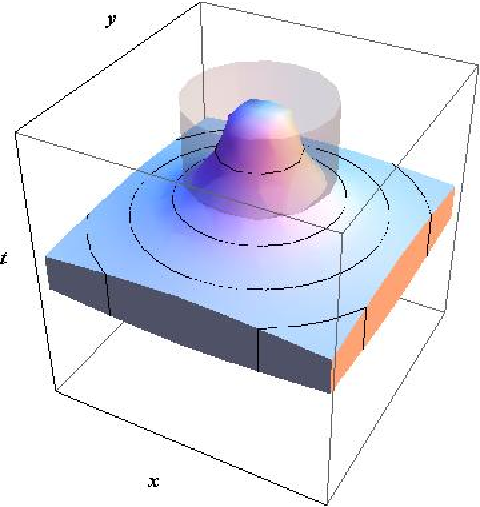
Now suppose that $\Sigma$ cannot be chosen to be bounded. For simplicity, we will assume that $\Sigma$ can be chosen so that it extends to spatial infinity in all directions. (We are ignoring the case where $\Sigma$ is unbounded, but not necessarily in all directions. The argument given here is intended to be representative: it can be extended to include these more complicated cases by, for instance, choosing $O$ so that the temporal height of its closure would vanish at any boundary of $\Sigma$.) Choose $O$ so that it has the following property: in the limit of spatial infinity, the “temporal height” of $O$ goes to zero (see Fig. 1). Here is one way (of many) to make this idea precise. Without loss of generality, choose the time function $t$ so that for any $s\in I$, $t(\gamma(s))=0$. Let $\varpi$ be any (fixed) timelike geodesic passing through $\Sigma$. Then given any point $p$ in a spacelike hypersurface intersecting $\varpi$, we can define a distance function $d:M\rightarrow\mathbb{R}$ relative to $\varpi$ as the (spatial) distance from $\varpi$ to $p$. We can then define an open set $O=\{p\in M|\text{ }|t(p)|<a\text{ and }|d(p)t(p)|<1\}$, for some constant real number $a$ chosen so that $\varpi$ intersects all of the simultaneity slices of $M$ with time values from $-a$ to $a$. Note first that $\Sigma\subset O$, so $\gamma[I]\subset O$. Moreover, for any $p\in O-\Sigma$, there exists a spacelike hypersurface $\Sigma^{\prime}$ for which $p\in\Sigma^{\prime}$ and $\Sigma^{\prime}$ slices $O$ (since the restriction of $O$ to any spacelike hypersurface except $\Sigma$ is bounded by construction).

From here the argument is similar to the bounded case. For any given $a$, there exist spacelike hypersurfaces $\Sigma_{\pm}$ such that for any $p\in\Sigma_{+}$, $t(p)>a$, and for any $p\in\Sigma_{-}$, $t(p)<-a$. These are necessarily such that $\Sigma_{\pm}\cap O=\emptyset$. It follows that $T^{ab}$ vanishes on $\Sigma_{\pm}$, and thus that $P^{a}(\Sigma_{\pm})=\mathbf{0}$ (where the integrals are performed relative to the arbitrary flat derivative operator $\overset{f}{\nabla}$). Thus $P^{a}(\Sigma_{\pm})t_{a}=0$. Meanwhile, we know there must be some point $p\in O$ at which $T^{ab}\neq\mathbf{0}$. We can freely suppose that $t(p)\neq 0$ (because if $t(p)=0$, there necessarily exists a neighborhood around $p$ in which $T^{ab}\neq\mathbf{0}$, since $T^{ab}$ is smooth, and which must include points whose time values are greater and less than 0). Suppose without loss of generality that $t(p)>0$ (if $t(p)<0$, simply reverse the temporal order of the ensuing argument—we have already chosen $O$ so that there are temporally prior, non-intersecting spacelike hypersurfaces). Since $p\in O-\Sigma$, we know there’s a spacelike hypersurface $\Sigma^{\prime}$ that contains $p$ and slices $O$. By the mass condition and the smoothness of $T^{ab}$, we know that $P^{a}(\Sigma^{\prime})t_{a}>0$. Now we can use Stokes’ theorem as immediately above by connecting $\Sigma^{\prime}$ and $\Sigma_{+}$ to reason to a contradiction. Thus $\gamma$ cannot be spacelike.

Case 3: So far we have shown that if $\gamma$ is everywhere timelike then it must be (reparametrizable as) a geodesic, and that $\gamma$ cannot be everywhere spacelike. The final case concerns curves that are sometimes timelike and sometimes spacelike. Given case 1, it is sufficient to show that if $\gamma$ satisfies the assumptions of the theorem and is timelike at at least one point, then it is timelike everywhere. Suppose otherwise—i.e., suppose there is at least one point $q$ at which $\gamma$ is spacelike. Let $s_{1}\in I$ be such that $\gamma$ is timelike at $\gamma(s_{1})$ and let $s_{2}\in I$ be such that $\gamma$ is spacelike at $\gamma(s_{2})$. Let $\xi^{a}$ be the tangent field to $\gamma$. We can define a scalar field on $\gamma$ by $\alpha=\xi^{a}t_{a}$. $\alpha$ can be understood as a smooth function $\alpha:I\rightarrow\mathbb{R}$ defined by $\alpha(s)=\alpha\circ\gamma(s)=(\xi^{a}t_{a})_{|\gamma(s)}$. Since $\gamma$ is timelike at $\gamma(s_{1})$, we know that $\alpha(s_{1})>0$; likewise, since $\gamma$ is spacelike at $\gamma(s_{2})$, $\alpha(s_{2})=0$. Since $\alpha$ is just a smooth function on the reals, however, we know that there must be a number $t\in I$ such that $\alpha(t)>0$, but for which $\left(\frac{d}{ds}\alpha\right)(t)\neq 0$. But by definition of $\xi^{a}$, $\frac{d}{ds}\alpha(s)=(\xi^{a}{}_{|\gamma(s)})(\alpha)=\xi^{a}\nabla_{a}\alpha=t_{b}\xi^{a}\nabla_{a}\xi^{b}$. So at $\gamma(t)$, we know that $(t_{b}\xi^{a}\nabla_{a}\xi^{b})_{|\gamma(t)}\neq 0$, and that $\xi^{a}t_{a}>0$.

So $\gamma$ is timelike at $\gamma(t)$, which means (since $\gamma$ is smooth and imbedded) that there must be an open neighborhood $Q$ of $\gamma(t)$ such that the restriction of $\gamma[I]$ to $Q$ is timelike. (Why? Since $\gamma$ is smooth, there must be an open neighborhood $J\subseteq I$ of $t$ such that $\gamma[J]$ is timelike. And since $\gamma$ is imbedded, there must be an open subset $Q$ of $M$ such that $\gamma[J]=\gamma[I]\cap Q$. So the restriction of $\gamma[I]$ to $Q$ is timelike and contains $\gamma(t)$.) We can freely choose $Q$ so that it is simply connected. Note that since $\gamma$ is such that for any neighborhood of $\gamma$, there exists a smooth symmetric field $T^{ab}$ satisfying conditions 1-4, it follows that for any sub-neighborhood $Q^{\prime}$ of $Q$ containing $\gamma[I]\cap Q$, there also exists a smooth symmetric field $T^{ab}$ such that the restriction of $T^{ab}$ to $Q$ satisfies conditions 1-4, relative to $Q^{\prime}$. (Why? Extend $Q^{\prime}$ to a neighborhood $O$ of all of $\gamma$ in any way at all, so long as $O\cap Q=Q^{\prime}$. Then a field $T^{ab}$ satisfying conditions 1-4 relative to $O$ is guaranteed to exist by the assumptions of the theorem; the restriction of $T^{ab}$ to $Q$ automatically inherits conditions 1-3. And by the conservation of mass argument given in Lemma III.3, if $T^{ab}$ is non-vanishing anywhere within $O$, as it must be, then it is possible to show by a series of flux integrals that it is non-vanishing along the length of the curve, and so $T^{ab}$ must be non-vanishing somewhere in $Q^{\prime}$.) But then if we take $Q$ as a submanifold of $M$ and take the restriction of $\gamma$ to $Q$ as a timelike curve, case 1 applies and $\gamma$ must be a geodesic everywhere in $Q$. It follows that at $\gamma(t)\in Q^{\prime}$, $(\xi^{a}\nabla_{a}\xi^{b})_{\gamma(t)}=0$, which is a contradiction (since we showed that $(t_{b}\xi^{a}\nabla_{a}\xi^{b})_{|\gamma(t)}\neq 0$). And so $\gamma$ must be timelike everywhere.   $\square$

Mathematically, theorem III.4 differs from the Geroch-Jang theorem in at least two ways. First, it requires a curvature condition: $R^{ab}{}_{cd}=\mathbf{0}$. This condition enters the discussion via Lemma III.2, where the flat derivative operator used in the proof of Theorem III.4 is shown to exist. Our method for constructing a flat derivative operator requires the existence of a rigid, non-rotating timelike field (a field $\eta^{a}$ such that $\nabla^{a}\eta^{b}=\mathbf{0}$). The (local) existence of such a field in a spatially flat ($R^{abcd}=\mathbf{0}$) classical spacetime is in fact equivalent to $R^{ab}{}_{cd}=\mathbf{0}$. Thus, without the curvature condition, our construction fails. That said, it is quite likely (we believe) that a different argument can be given to show that an appropriate derivative operator does exist more generally, in which case it would be possible to relax the curvature condition in Theorem III.4.

To evaluate whether this curvature condition is a defect of the present argument, however, one needs to consider the status of this condition in the context of the geometrized Newtonian gravitation. The condition is necessary to recover standard Newtonian gravitation from the geometrized theory (see appendix A). Without it, it is possible to find a more general “Newtonian” theory (see Künzle [14], Ehlers [13], Malament [9]), but with a vector potential replacing the scalar potential of standard Newtonian gravitation, and with a universal rotation field affecting the behavior of this vector potential. We would like to note, however, that insofar as we were interested in the status of the geodesic principle in Newtonian physics (rather than in some generalized Newtonian physics), $R^{ab}{}_{cd}=\mathbf{0}$ is a perfectly reasonable requirement: it holds just in case a geometrized Newtonian spacetime admits a standard Newtonian representation. It is part of what makes a classical spacetime Newtonian.

The second difference is that the present result assumes the underlying manifold $M$ be simply connected; the Geroch-Jang theorem, however, does not seem to require any such global topological assumptions. The reason that simple-connectedness is required here is that vector integration in a classical spacetime, at least as we have developed it, requires simple connectedness to ensure a unique result for the integral (since otherwise, parallel transport is not necessarily globally unique). Geroch and Jang use Killing fields to avoid this problem entirely; however, in a classical spacetime one does not have access to timelike Killing fields, even locally or in flat spacetime. However, there is a simple corollary available that (partially) extends the result to a more general case.

Corollary IV.1 precisifies a sense in which local geodesic motion has the status of a general theorem in geometrized Newtonian gravitation even in the absence of general topological assumptions.

References

- [1] A. Einstein, L. Infeld, and B. Hoffman, “The gravitational equations and the problem of motion,” Annals of Mathematics 39, 65–100 (1938).
- [2] T. Y. Thomas, “On the geodesic hypothesis in the theory of gravitation,” Proceedings of the National Academy of the USA 48, 1567–1569 (1962).
- [3] A. H. Taub, “On thomas’ result concerning the geodesic hypothesis,” Proceedings of the National Academy of the USA 48, 1570–1571 (1962).
- [4] W. G. Dixon, “A covariant multipole formalism for extended test bodies in general relativity,” Il Nuovo Cimento 34, 317–339 (1964).
- [5] J.-M. Souriau, “Modèle de particule à spin dans le champ électromagnétique et gravitationnel,” Annales de l’Institut Henri Poincaré Sec. A 20, 315 (1974).
- [6] S. Sternberg and V. Guillemin, Symplectic Techniques in Physics (Cambridge University Press, Cambridge, 1984).
- [7] R. Geroch and P. S. Jang, “Motion of a body in general relativity,” Journal of Mathematical Physics 16, 65 (1975).
- [8] J. Ehlers and R. Geroch, “Equation of motion of small bodies in relativity,” Annals of Physics 309, 232–236 (2004).
- [9] D. B. Malament, Topics in the Foundations of General Relativity and Newtonian Gravitation Theory (University of Chicago Press, Chicago, 2011) forthcoming.
- [10] E. Cartan, “Sur les variétés à connexion affine, et la théorie de la relativité généralisée (première partie),” Annales scientifiques de l’École Normale Supérieure 40, 325–412 (1923).
- [11] E. Cartan, “Sur les variétés à connexion affine, et la théorie de la relativité généralisée (première partie) (suite),” Annales scientifiques de l’École Normale Supérieure 41, 1–25 (1924).
- [12] K. O. Friedrichs, “Eine invariante formulierun des newtonschen gravitationsgesetzes und der grenzüberganges vom einsteinschen zum newtonschen gesetz,” Mathematische Annalen 98, 566–575 (1927).
- [13] J. Ehlers, “über den newtonschen grenzwert der einsteinschen gravitationstheorie,” in Grundlagen Probleme der Modernen Physik, edited by J. Nitsch, J. Pfarr, and E.-W. Stachow (Bibliographisches Institut, Zurich, 1981).
- [14] H. P. Künzle, “Covariant newtonian limit of lorentz space-times,” General Relativity and Gravitation 7, 445–457 (1976).
- [15] A. Trautman, “Foundations and current problem of general relativity,” in Lectures on General Relativity, edited by S. Deser and K. W. Ford (Prentice-Hall, Englewood Cliffs, NJ, 1965).
- [16] C. Duval and H. P. Künzle, “Dynamics of continua and particles from general covariance of newtonian gravitation theory,” Reports on Mathematical Physics 13 (1978).
- [17] At least, the Geroch-Jang theorem and Theorem III.4 of this paper are directly parallel mathematically. There is a second kind of question that one might ask, concerning the interpretations of the two theorems in the contexts of their respective spacetime theories. For instance, one might wonder if the conservation condition is as natural an assumption in geometrized Newtonian gravitation as in GR. We do not address such questions here, but will return to them in future work.
- [18] Modified because by our definition, does not slice the support of , since . But in this special case the argument still goes through.
- [19] This notation may require explanation. Briefly, if is a derivative operator on , then any other derivative operator on is determined relative to by a smooth symmetric (in the lower indices) tensor field, , and so specifying the field and is sufficient to uniquely determine a new derivative operator.
- [20] R. V. Benson, Euclidean geometry and convexity (McGraw-Hill, New York, 1966).