The Dynamics of Semilattice Networks
Abstract.
Time-discrete dynamical systems on a finite state space have been used with great success to model natural and engineered systems such as biological networks, social networks, and engineered control systems. They have the advantage of being intuitive and models can be easily simulated on a computer in most cases; however, few analytical tools beyond simulation are available. The motivation for this paper is to develop such tools for the analysis of models in biology. In this paper we have identified a broad class of discrete dynamical systems with a finite phase space for which one can derive strong results about their long-term dynamics in terms of properties of their dependency graphs. We classify completely the limit cycles of semilattice networks with strongly connected dependency graph and provide polynomial upper and lower bounds in the general case.
1. Introduction and Background
Time-discrete dynamical systems on a finite state space play an important role in several different contexts. Examples of such systems include Boolean networks, cellular automata, agent-based models, and finite state machines, to name a few. This modeling paradigm has been used with great success to model natural and engineered systems such as biological networks, social networks, and engineered control systems. It has the advantage of being intuitive and models can be easily simulated on a computer in most cases. A disadvantage of discrete models of this type is that few analytical tools beyond simulation are available. The motivation for this paper is to develop such tools for the analysis of models in biology, but the results are of independent mathematical interest. Some theoretical results have been proven for Boolean networks and are reviewed in [7]. In that paper the authors study conjunctive Boolean networks, that is, Boolean networks for which the future state of each node is computed using the Boolean AND operator. It is shown that the dynamics of such networks is controlled strongly by the topology of the network. The current paper shows that the results in [7] are valid much more broadly. We briefly describe the main results in [7].
A Boolean network on nodes can be viewed as a time discrete dynamical system over the Boolean field :
where the coordinate functions are the Boolean functions assigned to the nodes of the network. We can associate two directed graphs to . The dependency graph (or wiring diagram) of has vertices corresponding to the variables of . There is a directed edge if the function depends on (i.e. there is an instance where changing the value of changes the value of ). That is, encodes the variable dependencies in . The dynamics of is encoded by its phase space, denoted by . It is the directed graph with vertex set and a directed edge from to if . Thus, the graph encodes part of the structure of and the graph encodes its dynamics. The results in [7] relate these two graphs, deriving information about from , in the case where each is a conjunction of the variables for which there is an edge in . These networks were called conjunctive networks in [7].
It is easy to see that the graph has the following structure. Its connected components consist of a unique directed cycle, a limit cycle, with directed “trees” feeding into the nodes of the cycle, representing the transient states of the network, each of which eventually maps to a periodic point. If the graph is strongly connected, that is, there is a directed path from any vertex to any other vertex, then it is shown in [7] that there is a precise closed formula for the number of limit cycles of any given length. This formula depends on a numerical invariant of , its loop number. If is not strongly connected, then there is a sharp lower bound and an upper bound on the number of limit cycles, in terms of the loop numbers of the strongly connected components of and the antichains in the poset of strongly connected components. These two bounds agree for the number of fixed points of , so that one corollary is a closed formula for the number of fixed points of a general conjunctive network.
The current paper shows that these results hold in much broader generality, namely for time discrete dynamical systems over any finite set :
such that the are constructed from an operator , which has the property that it endows with the structure of a semilattice, that is, is commutative, associative, and idempotent. We will call such functions semilattice functions. That is, any semilattice gives rise to a dynamical system to which the formulas and bounds for limit cycles hold. It is shown furthermore that they hold precisely for the class of semilattice networks. It is important to mention that since semilattice networks are not linear (see Example 6.1), our results complement those for linear systems in [3, 5].
2. Semilattice networks
Let be a set with elements and consider a dynamical system with variables over :
Definition 2.1.
A function is called a semilattice operator if it satisfies the following (with notation ):
Note that semilattice operators induce the structure of a semilattice on . Conversely, the meet or join operations on a semilattice are semilattice operators in the above sense.
Example 2.2.
Some examples of semilattice operators are:
That is, semilattice operators are a generalization of the conjunctive and disjunctive operators used in [7].
The domain of a semilattice operator can be extended to with by
We will call such an extended operator a semilattice function.
Definition 2.3.
A dynamical system is called a semilattice network if there exists a semilattice operator, , such that is a semilattice function for all (where depends only on ).
Let be a semilattice network, , and the adjacency matrix of . We will assume here and in the remainder of the paper that none of the coordinate functions of are constant, that is, all vertices of have positive in-degree.
2.1. Structure of the Dependency Graph
Define the following relation on the vertices of : if and only if there is a directed path from to and a directed path from to . It is easy to check that is an equivalence relation. Suppose there are equivalence classes . For each equivalence class , the subgraph with the vertex set is called a strongly connected component of . The graph is called strongly connected if consists of a unique strongly connected component. A trivial strongly connected component is a graph on one vertex and no self loop. Since such components do not influence the cycle structure of the network, we assume that all strongly connected components are non-trivial.
Example 2.4.
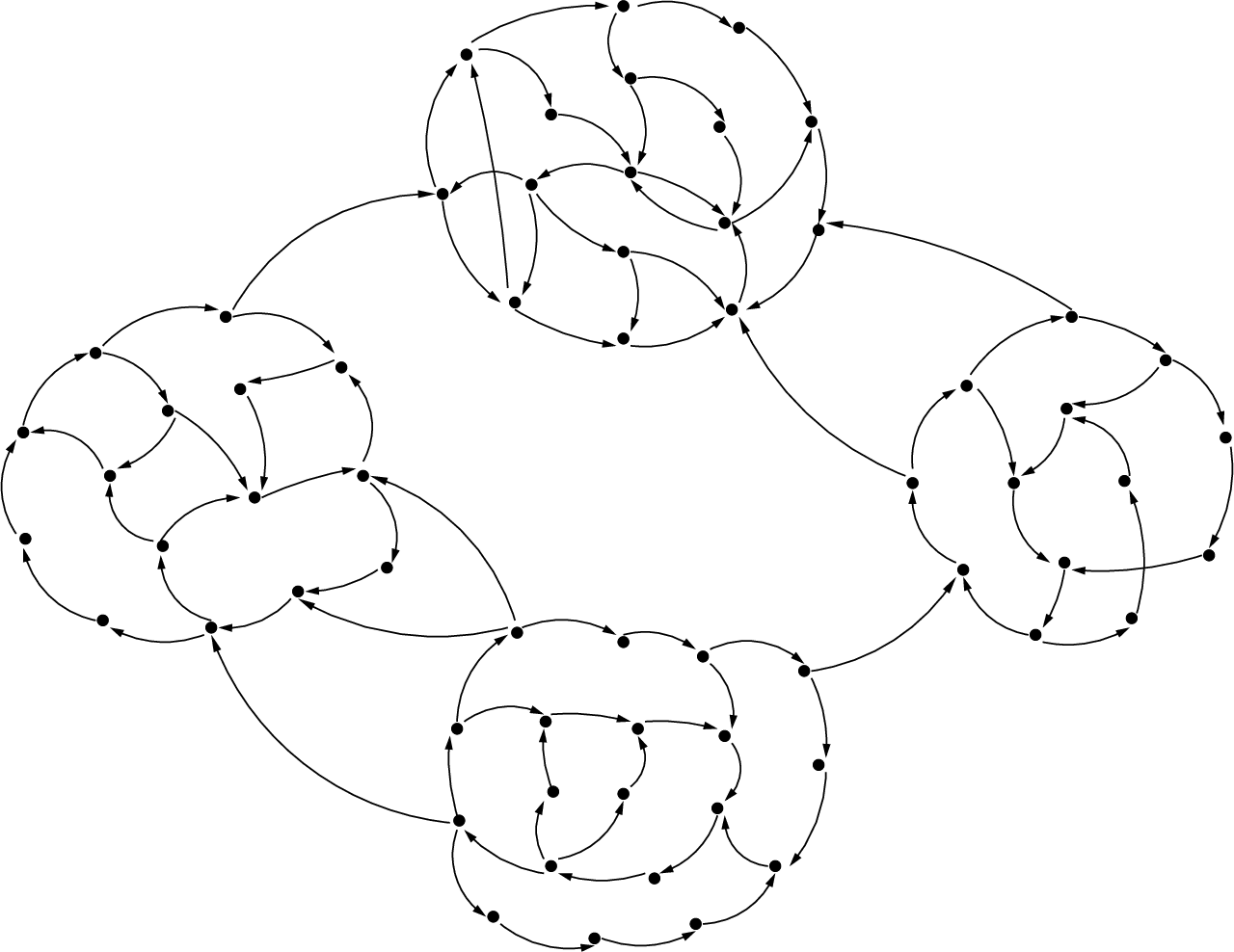
Our running example for this paper will be the semilattice network with dependency graph given by Figure 1 and semilattice function .
Let be a strongly connected component, and let be the semilattice network with dependency graph . Let be the semilattice network defined by . That is, the dependency graph of is the disjoint union of the strongly connected graphs , and is obtained from by deleting all edges between strongly connected components.
Now define the following order relation on the strongly connected components of the dependency graph of the network .
| (2.1) |
In this way we obtain a partially ordered set . In this paper, we relate the dynamics of to the dynamics of its strongly connected components and the poset .
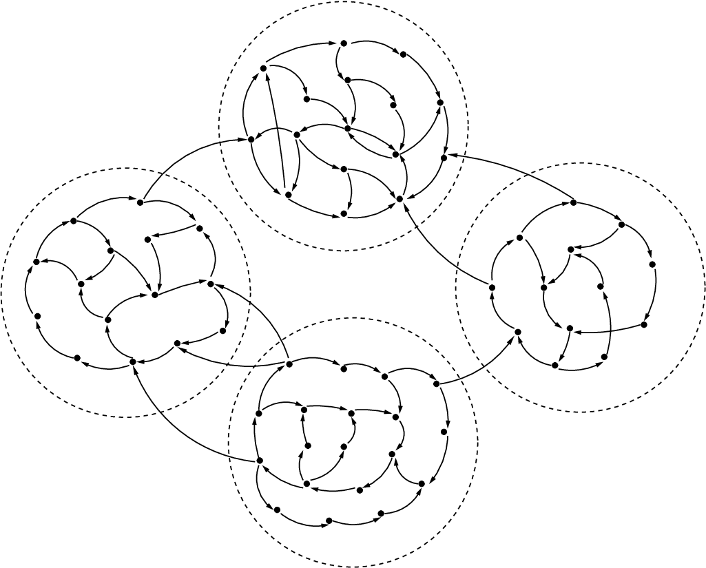
Example 1 (Cont.). The dependency graph of has four strongly connected components, , , , and (bottom, left, right and top, resp.). The poset is given by .

2.2. The Loop Number
Definition 2.5.
The loop number of a strongly connected graph is the greatest common divisor of the lengths of its simple (no repeated vertices) directed cycles. The loop number of any directed graph is the least common multiple of the loop numbers of its non-trivial strongly connected components.
Example 1 (Cont.). In our running example, the loop numbers are , , and .
3. Semilattice Networks with Strongly Connected Dependency Graph
In this section we give an exact formula for the cycle structure of semilattice networks with strongly connected dependency graphs. In the next section we will also consider networks with general dependency graphs and give upper and lower bounds for the cycle structure.
The formula for conjunctive networks was given and proven in [7]. It is not difficult to show that the proofs are also valid for general semilattice networks.
Let be a semilattice network with semilattice operator . Assume that the dependency graph of is strongly connected with loop number .
Lemma 3.1.
The set of vertices of can be partitioned into non-empty sets such that each edge of is an edge from a vertex in to a vertex in for some with and .
Let be the number of elements of . Without loss of generality we assume for the rest of the section that , ,…, ,
Proposition 3.2.
Let be the loop number of ; then there exists such that for all we have
where
Proof.
The proof is analogous to [2, Theorem 4.10]. ∎
The following corollary states that the period of can be obtained from the topology of its dependency graph.
Corollary 3.3.
The period of is equal to the loop number of .
The following corollary states that the long-term dynamics of a semilattice network can be reduced to the dynamics of a rotation over , with as in Lemma 3.1.
Corollary 3.4.
The cycle structure of is equal to the cycle structure of where .
Proof.
Let and be defined by and . The proof now follows from the equalities and . ∎
For any positive integers that divide , let be the set of periodic points of period and let .
Proposition 3.5.
The cardinality of the set is .
Proof.
It follows from the fact that if , then a rotation in colors and variables has colorings of periods that divide . ∎
Corollary 3.6.
If is a prime number and divides for some , then
Proof.
It is clear that (there are constant colorings). Now if is prime and , then the proof follows from the fact that , where is the disjoint union. ∎
Next we prove Theorem 3.7 which gives the exact number of periodic points of any possible length.
Theorem 3.7.
Let be a semilattice network whose dependency graph is strongly connected and has loop number . If , then . If and is a divisor of , then the number of periodic states of period is
| (3.1) |
Proof.
The statement for is part of the previous corollary. Now suppose that . For , let . Then , where is a disjoint union, in particular,
The formula 3.1 follows from the inclusion-exclusion principle and the disjoint union above. ∎
Corollary 3.8.
If divides , then the number of cycles of length in the phase space of is . Hence the cycle structure of is
Example 1 (Cont.). In our running example we obtain:
Remark 3.9.
Notice that the cycle structure of depends on the loop number and only. In particular, a semilattice network with loop number 1 on a strongly connected dependency graph only has as limit cycles the fixed points where , regardless of how many vertices its dependency graph has and how large is.
4. Networks with general dependency graph
Let be a semilattice network with dependency graph . Let be the strongly connected components of . Furthermore, suppose that none of the is trivial. For , let be the semilattice network that has as its dependency graph and suppose that the loop number of is . In particular, the loop number of is .
First we study the effect of deleting an edge in the dependency graph between two strongly connected components. Let and be two strongly connected components in and suppose . Let be a directed edge in between a vertex in and a vertex in . Let be the graph after deleting this edge, and let be the semilattice network such that .
Theorem 4.1.
Any cycle in the phase space of is a cycle in the phase space of . In particular componentwise.
Proof.
First notice that appears in the expression if and only if there is a path from to of length . Let be a cycle of length in . To show that is a cycle in , it is enough to show that, . Thus, the value of is determined already by the value of and the edge does not contribute anything new and hence is a cycle in . This is equivalent to show that for all such that there is an edge from to .
Suppose the loop number of (resp. ) is (resp. ). Now, any path from (resp. ) to itself is of length (resp. ) where and is large enough, see [2, Corollary 4.4]. Thus there is a path from to of length for any . Also, there is a directed path from to of length for any . This implies the existence of a path from to of length for all , then appears in .
Now , for all . Choose large enough such that . Then, and . Therefore . ∎
Let be the semilattice network with the disjoint union of as its dependency graph. That is, . For , there are no edges between any two strongly connected components of the dependency graph of the network. Its cycle structure can be completely determined from the cycles structures of the alone.
Theorem 4.2.
Let be the cycle structure of . Then the cycle structure of is (where ) and the number of cycles of length (where ) in the phase space of is
| (4.1) |
Proof.
This follows from the fact that if is a periodic point of of period and is a periodic point of of period , then is a periodic point of of period . ∎
Corollary 4.3.
Let and be as above. The number of cycles of any length in the phase space of is less than or equal to the number of cycles of that length in the phase space of . That is componentwise. In particular, the period of is a divisor of the loop number of its dependency graph.
In [7], it was shown that the poset structure of gives an algebraic way to combine the cycle structure of to obtain lower and upper bounds for the cycle structure of , where was a conjunctive Boolean network. It is not difficult to see that the proofs of these results still also hold for general semilattice networks if the corresponding semilattice operator has a “neutral” and an “absorbent” element (analogous to the identities and ). In order to state the theorem about lower and upper bounds of semilattice networks, we need the following definitions.
Definition 4.4.
Let be a semilattice operator. An element is called a neutral element if for all . An element is called an absorbent element if for all .
Example 4.5.
All the functions in Example 2.2 have a neutral and absorbent element; they are:
| , | ||||
| , | ||||
| , | ||||
| , |
Remark 4.6.
Since is finite, every semilattice operator has an absorbent element ().
Remark 4.7.
Any semilattice operator on can be extended to a set with a neutral element by defining as if and otherwise.
Let , , be as above and let be the loop number of . Furthermore, let be the poset of the strongly connected components. Let be the set of all maximal antichains in . For , let and let . In the remainder of the paper we assume that is a semilattice network such that its semilattice operator, , has idempotent neutral and absorbent elements, and , resp.
Definition 4.8.
For any subset , let
A limit cycle in the phase space of is (resp. ) if the component of is (resp. ) for all .
Denote and .
Definition 4.9.
The - and -polynomial associated to are defined as follows:
Theorem 4.10.
With the notation above we have the following coefficient-wise inequalities
Here, the polynomials and are evaluated using the “multiplication” described in Theorem 4.2 and coefficient-wise addition.
Proof.
The proof is analogous to the proofs of Theorems 6.2 and 7.4 in [7]. ∎
Note that the left and right sides of the inequalities (4.10) are polynomial functions in the variables , with integer coefficients. That is, the lower and upper bounds are polynomial functions depending exclusively on measures of the network topology.
Example 1 (Cont.). In our running example we obtain:
and therefore . It is important to mention that the phase space of has nodes so it is not feasible to obtain information about the cycle structure from exhaustive enumeration. Also, although the bounds agree on fixed points for Boolean semilattice networks [7], our example shows that they do not agree for general lattice networks.
5. Characterization of Semilattice Networks
In this section we characterize semilattice networks; in order to do this, it is enough to characterize semilattice operators. Since semilattice operators are semilattice operations, the number of semilattice operators over a set with elements (up to permutation) is the number of semilattices with elements. According to the next proposition, the number of semilattice operators over a set with elements is the number of lattices of size . Although there is no closed formula for the number of lattices of a given size, algorithms for counting them have been developed [4].
Proposition 5.1.
There is a one-to-one correspondence between semilattices with elements and lattices with elements.
Proof.
If is a semilattice with elements, consider , by defining if and otherwise; also, . It follows that is a lattice with elements. On the other hand, if is a lattice with elements, let ; then it follows that is a semilattice with elements. ∎
6. Infinite Semilattice Networks
We present some results on infinite semilattice networks, both networks on an infinite set and networks on an infinite Cartesian product of a set .
6.1. Semilattice networks on infinite sets
If is a set with infinitely many elements (that is, ), some of the theorems remain valid. Notice that if is finite, there exists a finite set that is closed under ; that is, is a semilattice function.
Suppose that is strongly connected with loop number , and let be a periodic point of . Let be a finite subset of that it is closed under ; then we can consider as a periodic point of . Therefore, the results on finite semilattice networks apply, and the period of must divide . That is, Corollary 3.3 is valid for . Now, consider a divisor of and consider finite with at least elements such that is a semilattice operator. Then, the number of periodic states of period of is at least (see Theorem 3.7 and notice that is increasing with respect to ). Since , it follows that has infinitely many periodic points and limit cycles of length . Then Theorem 3.7 (and the corresponding corollary) holds for .
If is not necessarily strongly connected, suppose has a neutral and an absorbent element. Let correspond to Then, by using the argument in the paragraph above, it follows that if at least a limit cycle of length appears in , then has infinitely many limit cycles of length .
6.2. Infinite-dimensional semilattice networks
If the dimension of is infinite, that is, , then needs to satisfy an additional condition to be properly defined: Every (possibly infinite) subset has a largest lower bound. This means that there exists such that for all (in lattice terminology: is a lower bound); and if there is another such , then (in lattice terminology: is the largest lower bound). This additional condition allows for a function to have infinitely many inputs.
Suppose that is strongly connected with loop number , and let be a periodic point of of period . Consider (see Lemma 3.1); then there exists such that for all there is a path of length from to and from to . Then, , for all ; in particular, and for some . Then, , similarly ; therefore . It follows that Corollary 3.3 and Theorem 3.7 remain valid for (and ).
If is not necessarily strongly connected, suppose has a neutral and an absorbent element. It is not difficult to show that Theorem 4.10 remains valid for (and ).
Finally, we show with counterexamples that we cannot omit any of the properties of in Definition 2.1. That is, the formulas and bounds derived in this paper are valid exactly for semilattice networks.
Example 6.1.
Consider , then is commutative and associative, but not idempotent. Consider , defined by . It is not difficult to see that has a unique limit cycle (a fixed point), ; that is, . On the other hand, the loop number of its dependency graph is , so from Theorem 3.7 we would obtain .
Example 6.2.
Consider defined over . It is easy to show that associative and idempotent, but not commutative. Consider , defined by . It is not difficult to show that has the limit cycle of length 2, (it also has 3 fixed points). On the other hand, the loop number of its dependency graph is , so from Theorem 3.7 we would obtain .
Example 6.3.
Consider defined over . It is easy to show that is commutative and idempotent, but not associative. Consider , defined by . It is not difficult to show that has the limit cycle of length 3, (it also has 3 fixed points and another limit cycle of length 3). On the other hand, the loop number of its dependency graph is , so from Theorem 3.7 we would obtain .
7. Discussion
In this paper we have identified a broad class of discrete dynamical systems with a finite phase space for which one can derive strong results about their long-term dynamics in terms of properties of their dependency graphs. We classify completely the limit cycles of semilattice networks with strongly connected dependency graph and provide polynomial upper and lower bounds in the general case. It is our hope that the formulas in this paper are related to general properties of semilattices, which is a subject for future investigation. As mentioned in the Introduction, the motivation for this investigation was the need for theoretical tools to analyze discrete models in biology. An example of such an application is given in [6], where it is shown that the results about conjunctive Boolean networks can be applied to determining the limiting behavior of certain types of epidemiological models.
The results in this paper apply to certain types of Boolean networks and cellular automata, which in many cases have the property that the update functions are of the same type for all nodes. Another model type to which the results in this paper apply in some cases is that of so-called logical models, developed by René Thomas for the purpose of modeling gene regulatory networks. It is shown in [8] that logical models can be translated into the framework of polynomial dynamical systems. If the dynamical system arises from a semilattice function, then the results of this paper give information about the steady states and limit cycles of the model under synchronous update.
References
- [1] R. A. Brualdi and H. J. Ryser, Combinatorial matrix theory, vol. 39 of Encyclopedia of Mathematics and its Applications, Cambridge University Press, Cambridge, 1991.
- [2] O. Colón-Reyes, R. Laubenbacher, and B. Pareigis, Boolean monomial dynamical systems, Annals of Combinatorics, 8 (2004), pp. 425–439.
- [3] B. Elspas, The theory of autonomous linear sequential networks, IRE Transaction on Circuit Theory, (1959), pp. 45–60.
- [4] J. Heitzig and J. Reinhold, Counting finite lattices, Algebra Universalis, 48 (2002), pp. 43–53.
- [5] A. Hernández-Toledo, Linear finite dynamical systems, Communications in Algebra, 33 (2005), pp. 2977–2989.
- [6] F. Hinkelmann, D. Murragarra, A. Jarrah, and R. Laubenbacher, A mathematical framework for agent based models of complex biological networks, (2010), p. arXiv:1006.0408.
- [7] A. S. Jarrah, R. Laubenbacher, and A. Veliz-Cuba, The dynamics of conjunctive and disjunctive boolean network models, Bull. Math. Bio., (2010).
- [8] A. Veliz-Cuba, A. Jarrah, and R. Laubenbacher, Polynomial algebra of discrete models in systems biology, Bioinformatics, 26 (2010), pp. 1637–1643.