跳到论文正文
W Papers独立论文阅读器 arXiv:1010.0348 论文正文 计算阅读时间 · 0%
引用这篇论文根据当前论文元数据生成,正式投稿前建议核对。


License: arXiv.org perpetual non-exclusive license
arXiv:1010.0348v2 [hep-th] 16 Mar 2011

Refined Wall-Crossing, Free Fermions and Crystal Melting

Haitao Liu 1, and Jie Yang2

1 Department of Mathematics and Statistics, University of New Brunswick, Fredericton, Canada

and

Theoretical Physics Group, The Blackett Laboratory, Imperial College London, London, UK

and

Department of Applied Mathematics, Hebei University of Technology, Tianjin, China

haitao.liu@unb.ca

2 School of Mathematical Sciences, Capital Normal University, Beijing, China

and

SISSA, INFN, Sezione di Trieste, via Bonomea 265, Trieste, Italy

yang9602@gmail.com

ABSTRACT

In this paper, we use an M-theory model to conjecture the refined reminiscence of the OSV formula connecting the refined topological string partition function with the refined BPS states partition function for the toric Calabi-Yau threefolds without any compact four cycles. Further, we show how to use the vertex operators in 2d free fermions to reproduce the refined BPS states partition function for the ℂ3\mathbb{C}^{3} case and the wall-crossing formulas of the refined BPS states partition function for the resolved conifold and 𝒪⁡(−2)⊕𝒪→ℙ1\mathcal{O}(-2)\oplus\mathcal{O}\rightarrow\mathbb{P}^{1} cases.

1 Introduction

Recent years people have made lots of progress on understanding the space of BPS states, ℋB​P​S\mathcal{H}_{BPS}, in type II string compactifications on Calabi-Yau threefolds. In general, such compactifications give rise to the effective 𝒩=2\mathcal{N}=2 theories in four dimensions. ℋB​P​S\mathcal{H}_{BPS} is a special subspace of the full Hilbert space which is the one-particle representation of the d=4,𝒩=2d=4,\mathcal{N}=2 supersymmetry algebra. In fact, the space ℋB​P​S\mathcal{H}_{BPS} contains lots of information about the Calabi-Yau threefold XX. It is a bridge connecting the black hole physics and topological strings [1].

In fact, the space ℋB​P​S\mathcal{H}_{BPS} is graded by charge sectors

ℋB​P​S=⊕γ∈ΓℋB​P​S(γ),\mathcal{H}_{BPS}=\oplus_{\gamma\in\Gamma}\mathcal{H}_{BPS}(\gamma), (1.1)

where Γ\Gamma denotes the charge lattice. According to [2, 3, 4] in the Calabi-Yau compactification of type IIA string theory, the lattice Γ\Gamma is given by the cohomology of the Calabi-Yau threefold Γ=Heven​(X,ℤ)\Gamma=\text{H}^{\text{even}}(X;\mathbb{Z}), and γ\gamma is given by the generalized Mukai vector of the stable coherent sheaves corresponding to the D6/D4/D2/D0 branes

γ=c​h​(ℰ)​A^​(X)=p0+P+Q+q0∈H0⊕H2⊕H4⊕H6D​6D​4D​2D​0\begin{array}[]{ccccccccc}\gamma=ch(\mathcal{E})\sqrt{\hat{A}(X)}&=&p^{0}&+&P&+&Q&+&q_{0}\\ &\in&\text{H}^{0}&\oplus&\text{H}^{2}&\oplus&\text{H}^{4}&\oplus&\text{H}^{6}\\ &&D6&&D4&&D2&&D0\end{array} (1.2)

Further, ℋB​P​S​(γ)\mathcal{H}_{BPS}(\gamma) has the following decomposition due to the existence of the universal hypermultiplets

ℋB​P​S​(γ)=(𝟎,𝟎,𝟏𝟐)⊗ℋB​P​S′​(γ).\mathcal{H}_{BPS}(\gamma)=(\mathbf{0},\mathbf{0};\mathbf{\frac{1}{2}})\otimes\mathcal{H}^{\prime}_{BPS}(\gamma). (1.3)

In this paper we will focus on the reduced space ℋB​P​S′\mathcal{H}^{\prime}_{BPS}. It is well known that the space ℋB​P​S′\mathcal{H}^{\prime}_{BPS} depends on the asymptotic boundary conditions in the four-dimensional spacetime, where the boundary conditions in IIA compactification are the complexified Kähler moduli u=i​J+Bu=iJ+B of the Calabi-Yau threefold XX [4]. Roughly speaking, ℋB​P​S′​(γ,u)≅H∗​(ℳ⁡(γ,u))\mathcal{H}^{\prime}_{BPS}(\gamma,u)\cong\text{H}^{*}(\mathcal{M}(\gamma,u)), where ℳ⁡(γ,u)\mathcal{M}(\gamma,u) is the moduli space of the stable coherent sheaf with the generalized Mukai vector γ\gamma under certain uu-dependent stability condition [5]. Further, on ℋB​P​S\mathcal{H}_{BPS} there is an Spin(3) action, which gives rise to the following index of the ℋB​P​S′\mathcal{H}^{\prime}_{BPS} [6, 4]

Ω⁡(γ,u):=TrℋB​P​S′​(γ,u)​(−1)2​J3′,\Omega(\gamma,u):={\rm Tr}_{{\cal H}_{BPS}^{\prime}(\gamma,u)}(-1)^{2J_{3}^{\prime}}, (1.4)

where J3′J_{3}^{\prime} is the reduced angular momentum [4]. From the mathematical point of view, the index Ω⁡(γ,u)\Omega(\gamma,u) is related to the Euler characteristic of the space ℋB​P​S′​(γ,u)\mathcal{H}^{\prime}_{BPS}(\gamma,u). The interesting phenomenon is that the index Ω⁡(γ,u)\Omega(\gamma,u) is piecewisely constant with respect to uu. In other words, on the moduli space uu there are some chambers which split the moduli space into some small chambers. When we enter a new chamber crossing a wall, the index Ω⁡(γ,u)\Omega(\gamma,u) will jump to another integer. The detailed wall-crossing formulas of Ω⁡(γ,u)\Omega(\gamma,u) have been well understood for many cases [4, 7, 8, 9, 10, 11] etc. Notice that the index Ω⁡(γ,u)\Omega(\gamma,u) is only related to the Euler characteristic of the space ℋB​P​S′​(γ,u)\mathcal{H}^{\prime}_{BPS}(\gamma,u). Therefore we want to know how the cohomology jumps when we cross a wall. In [12], the authors defined the following refined index

Ωr​e​f​(γ,u,y):=TrℋB​P​S​(γ,u)′​(−y)2​J3′,\Omega^{ref}(\gamma,u,y):={\rm Tr}_{{\cal H}^{\prime}_{BPS(\gamma,u)}}(-y)^{2J_{3}^{\prime}}, (1.5)

where yy is a free parameter. Hence Ω⁡(γ,u,y)\Omega(\gamma,u,y) is a polynomial of yy. Thus we have

Ωr​e​f​(γ,u,y)→Ω⁡(γ,u) as ​y→1.\Omega^{ref}(\gamma,u,y)\rightarrow\Omega(\gamma,u)\ \ \text{ as }\ y\rightarrow 1. (1.6)

In [12], the authors claimed that the refined index Ωr​e​f​(γ,u,y)\Omega^{ref}(\gamma,u,y) is related to the q-deformed Motivic BPS index of Kontsevich and Soibelman in [13] via the following map

RefinedMotivicQuantumy↔𝕃12↔−q12\begin{array}[]{ccccccccc}\text{Refined}&&\text{Motivic}&&\text{Quantum}\\ y&\leftrightarrow&\mathbb{L}^{\frac{1}{2}}&\leftrightarrow&-q^{\frac{1}{2}}\end{array} (1.7)

They conjectured that in string theory on a Calabi-Yau threefold XX, the q-deformed motivic index of Kontsevich and Soibelman in [13] corresponds to turning on a graviphoton background on ℝ4\mathbb{R}^{4}. In particular, we have

Ωr​e​f​(γ,u,y)=Ωm​o​t​(γ,u)\Omega^{ref}(\gamma,u,y)=\Omega^{mot}(\gamma,u) (1.8)

with the appropriate identification of variables y,𝕃,qy,\mathbb{L},q.

Further, like the unrefined index we can define the refined BPS states partition function [12] by

𝒵B​P​Sr​e​f​(q,Q,y,u):=∑β∈H2​(X,ℤ)​n∈ℤ(−q)n​Qβ​Ωr​e​f​(γβ,n,u,y).\mathcal{Z}^{ref}_{BPS}(q,Q,y,u):=\sum_{\begin{subarray}{c}\beta\in\text{H}_{2}(X;\mathbb{Z})n\in\mathbb{Z}\end{subarray}}(-q)^{n}Q^{\beta}\Omega^{ref}(\gamma_{\beta,n},u,y). (1.9)

In [12], the author have shown how to use the dimer model to produce the wall-crossing formula of the refined BPS states partition function of the resolved conifold case. In this paper, we show how to use the vertex operators in 2d free fermions and the crystal corresponding to the Calabi-Yau threefold XX to reproduce the wall-crossing formula of the refined BPS states partition function.

Organization of the paper

In section 2, we conjecture the refined reminiscence of the OSV formula by using the M theory model; in section 3, we review some basic knowledge of the vertex operators in the two-dimensional free fermions; in section 4, we show how to use the vertex operators to produce the refined BPS states partition function on ℂ3{\mathbb{C}}^{3}; in section 5, we show how to use the vertex operators to reproduce the wall-crossing formulas of the refined BPS states partition function on the resolved conifold; in section 6, we show how to use the vertex operators to reproduce the wall-crossing formulas of the refined BPS states partition function on the 𝒪⁡(−2)⊕𝒪→ℙ1\mathcal{O}(-2)\oplus\mathcal{O}\rightarrow\mathbb{P}^{1}; in section 7, we discuss some possible future working directions.

2 Refined partition function of BPS states and refined reminiscence of the OSV formula

In [10], the authors employ the Taub-Nut space with the unit charge to lift the single D6 brane in type IIA theory to M-theory. Since the degeneracy of BPS states does not depend on the radius of the Taub-Nut circle, we can investigate the index of the BPS states in the large radius case, and then go back to the small radius case. Now let us focus on the large radius case in which the Taub-Nut becomes ℝ4{\mathbb{R}}^{4}. In other words, our 11-dimensional spacetime of M-theory is

X×ℝ4×S1,X\times{\mathbb{R}}^{4}\times S^{1}, (2.10)

where XX is a Calabi-Yau threefold and S1S^{1} is the time circle. Here we take the following assumptions which are the same as those in [10]:

  1. 1.

    Assume that the Kähler parameters of the Calabi-Yau are vanishing.

  2. 2.

    Assume that the only BPS states in 5D are particles.

The assumption 1 implies that the central charges of the BPS M2 branes are parallel; the assumption 2 implies that there are not any compact four-cycles in the Calabi-Yau threefold XX [10]. Therefore from now on when we use the symbol XX, it always refers to a Calabi-Yau threefold without any compact four-cycles.

Now let us consider the physics in the five-dimensional spacetime ℝ4×S1{\mathbb{R}}^{4}\times S^{1}. Since the isometry group of ℝ4{\mathbb{R}}^{4} is S​O​(4)=S​U​(2)L×S​U​(2)RSO(4)=SU(2)_{L}\times SU(2)_{R}, we have two kinds of internal spins: left one m1m_{1} and right one m2m_{2}. The U​(1)L×U​(1)R⊂S​U​(2)L×S​U​(2)RU(1)_{L}\times U(1)_{R}\subset SU(2)_{L}\times SU(2)_{R} action on ℝ4=ℂ2{\mathbb{R}}^{4}={\mathds{C}}^{2} is as follows

U​(1)L\displaystyle U(1)_{L} :\displaystyle: (z1,z2)↦(ei​ϵ1​z1,z2),\displaystyle(z_{1},z_{2})\mapsto(e^{i\epsilon_{1}}z_{1},z_{2}), (2.11)
U​(1)R\displaystyle U(1)_{R} :\displaystyle: (z1,z2)↦(z1,ei​ϵ2​z2),\displaystyle(z_{1},z_{2})\mapsto(z_{1},e^{i\epsilon_{2}}z_{2}), (2.12)

where z1,z2z_{1},z_{2} are the complex coordinates of ℂ2{\mathds{C}}^{2} and ei​ϵ1,ei​ϵ2e^{i\epsilon_{1}},e^{i\epsilon_{2}} are the generators of U​(1)L,U​(1)RU(1)_{L},U(1)_{R} actions respectively. Further, each five-dimensional BPS particle can have excitations on ℝ4=ℂ2{\mathbb{R}}^{4}={\mathds{C}}^{2}. These excitations can be expressed by holomorphic functions on ℂ2{\mathds{C}}^{2} [14, 10]:

Φβ,m1,m2​(z1,z2)=z1m1​z2m2​∑n1,n2≥0αβ,n1+m1,n2+m2​z1n1​z2n2,\Phi_{\beta,m_{1},m_{2}}(z_{1},z_{2})=z_{1}^{m_{1}}z_{2}^{m_{2}}\sum_{n_{1},n_{2}\geq 0}\alpha_{\beta,n_{1}+m_{1},n_{2}+m_{2}}z_{1}^{n_{1}}z_{2}^{n_{2}}, (2.13)

where z1,z2z_{1},z_{2} are the coordinates on ℂ2{\mathds{C}}^{2}, β∈H2​(X,ℤ)\beta\in H^{2}(X,{\mathbb{Z}}) is a curve class wrapped by the M2-brane, and αn1+m1,n2+m2\alpha_{n_{1}+m_{1},n_{2}+m_{2}} are bosonic or fermionic modes depending on whether the field Φ\Phi is bosonic or fermionic respectively. Denote by NβjL,jRN_{\beta}^{j_{L},j_{R}} the degeneracy of the five-dimensional BPS states of M2 branes of charge β\beta and left-right spin (jL,jR)(j_{L},j_{R}) under S​U​(2)L×S​U​(2)RSU(2)_{L}\times SU(2)_{R}. Then for each mode αβ,n1+m1,n2+m2\alpha_{\beta,n_{1}+m_{1},n_{2}+m_{2}} we have

2​jL3\displaystyle 2j_{L}^{3} =\displaystyle= n1+n2+m1+m2,\displaystyle n_{1}+n_{2}+m_{1}+m_{2}, (2.14)
2​jR3\displaystyle 2j_{R}^{3} =\displaystyle= n1−n2+m1−m2.\displaystyle n_{1}-n_{2}+m_{1}-m_{2}. (2.15)

Following [14, 15, 10], we may define the following unrestricted refined partition function:

𝒵F​o​c​k=TrF​o​c​k​(−1)2​(jL+jR)​q1jL3+jR3​q2jL3−jR3​e−T\displaystyle{\cal Z}_{Fock}=\text{Tr}_{Fock}(-1)^{2(j_{L}+j_{R})}q_{1}^{j_{L}^{3}+j_{R}^{3}}q_{2}^{j_{L}^{3}-j_{R}^{3}}e^{-T}
=\displaystyle= ∏β∈H2​(X,ℤ)∏jL,jR∏kL=−jL+jL∏kR=−jR+jR∏m1,m2=1∞(1−q1kL+kR+m1−12​q2kL−kR+m2−12​Qβ)(−1)2​(jL+jR)+1​NβjL,jR,\displaystyle\prod_{\beta\in H_{2}(X,{\mathbb{Z}})}\prod_{j_{L},j_{R}}\prod_{k_{L}=-j_{L}}^{+j_{L}}\prod_{k_{R}=-j_{R}}^{+j_{R}}\prod_{m_{1},m_{2}=1}^{\infty}(1-q_{1}^{k_{L}+k_{R}+m_{1}-\frac{1}{2}}q_{2}^{k_{L}-k_{R}+m_{2}-\frac{1}{2}}Q^{\beta})^{(-1)^{2(j_{L}+j_{R})+1}N_{\beta}^{j_{L},j_{R}}},

where q1=ei​ϵ1,q2=e−i​ϵ2,Q=e−Tq_{1}=e^{i\epsilon_{1}},q_{2}=e^{-i\epsilon_{2}},Q=e^{-T} and TT is the area of ℙ1\mathbb{P}^{1}. According to [14, 15, 16] the refined topological string partition function is defined by

𝒵t​o​pr​e​f=ℳ(q1,q2)Trℋ(−1)2​(jL+jR)q1jL3+jR3q2jL3−jR3e−T=ℳ(q1,q2)⋅\displaystyle{\cal Z}_{top}^{ref}=\mathcal{M}(q_{1},q_{2})\text{Tr}_{\cal H}(-1)^{2(j_{L}+j_{R})}q_{1}^{j_{L}^{3}+j_{R}^{3}}q_{2}^{j_{L}^{3}-j_{R}^{3}}e^{-T}=\mathcal{M}(q_{1},q_{2})\cdot
⋅∏β∈H2​(X,ℤ)β>0∏jL,jR∏kL=−jL+jL∏kR=−jR+jR∏m1,m2=1∞(1−q1kL+kR+m1−12​q2kL−kR+m2−12​Qβ)(−1)2​(jL+jR)+1​NβjL,jR,\displaystyle\cdot\prod_{\begin{subarray}{c}\beta\in H_{2}(X,{\mathbb{Z}})\\ \beta>0\end{subarray}}\prod_{j_{L},j_{R}}\prod_{k_{L}=-j_{L}}^{+j_{L}}\prod_{k_{R}=-j_{R}}^{+j_{R}}\prod_{m_{1},m_{2}=1}^{\infty}(1-q_{1}^{k_{L}+k_{R}+m_{1}-\frac{1}{2}}q_{2}^{k_{L}-k_{R}+m_{2}-\frac{1}{2}}Q^{\beta})^{(-1)^{2(j_{L}+j_{R})+1}N_{\beta}^{j_{L},j_{R}}},
(2.17)

where

ℳ⁡(q1,q2)=Mδ1(q1,q2)12⋯Mδχ⁡(X)(q1,q2)12⏟χ⁡(X)\mathcal{M}(q_{1},q_{2})=\underbrace{M_{\delta_{1}}(q_{1},q_{2})^{\frac{1}{2}}\cdots M_{\delta_{\chi(X)}}(q_{1},q_{2})^{\frac{1}{2}}}_{\chi(X)} (2.18)

and Mδ​(q1,q2)M_{\delta}(q_{1},q_{2}) is the refined MacMahon functions defined by

Mδ​(q1,q2)=∏i,j=1∞(1−q1i−12+δ2​q2j−12−δ2)−1,M_{\delta}(q_{1},q_{2})=\prod_{i,j=1}^{\infty}(1-q_{1}^{i-\frac{1}{2}+\frac{\delta}{2}}q_{2}^{j-\frac{1}{2}-\frac{\delta}{2}})^{-1}, (2.19)

χ⁡(X)\chi(X) is the Euler characteristic of the Calabi-Yau threefold XX, and δi\delta_{i} are constants related to how we setup the weight when we count the 3D Young diagrams [17, 12]. Thus we have the following equality:

𝒵F​o​c​k=𝒵t​o​pr​e​f​(q1,q2,Q)​𝒵t​o​pr​e​f​(q1,q2,Q−1).{\cal Z}_{Fock}={\cal Z}_{top}^{ref}(q_{1},q_{2},Q){\cal Z}_{top}^{ref}(q_{1},q_{2},Q^{-1}). (2.20)

Hence we may conjecture the following formula:

𝒵B​P​Sr​e​f​(c​h​a​m​b​e​r)=𝒵F​o​c​k|c​h​a​m​b​e​r=𝒵t​o​pr​e​f​(q1,q2,Q)​𝒵t​o​pr​e​f​(q1,q2,Q−1)|c​h​a​m​b​e​r.{\cal Z}_{BPS}^{ref}(chamber)={\cal Z}_{Fock}|_{chamber}={\cal Z}_{top}^{ref}(q_{1},q_{2},Q){\cal Z}_{top}^{ref}(q_{1},q_{2},Q^{-1})|_{chamber}. (2.21)

We call it the refined reminiscence of the OSV formula 44 4 We owe this clarification to M. Yamazaki.. Here we need to clarify the meaning of a chamber. The chambers here are supposed to be the same as the chambers in the unrefined case. Since the refined wall-crossing formulas are dealing with the Poincaré polynomial of the BPS states moduli space, the wall of the unrefined BPS states partition function must be the wall of the refined BPS partition. But the question here is if there exist some invisible walls beyond the walls in the unrefined case? The answer is negative. In other words, if the refined reminiscence of the OSV formula (2.21) is true then there do not exist any invisible walls, since if the chamber of the Euler characteristic is fixed then the right hand side of the formula (2.21) is fixed. It implies that if there exists an invisible wall splitting the chamber into two smaller chambers, then the right hand side of the formula (2.21) can NOT distinguish these two smaller chambers, which implies that the expression of the left hand side of the formula (2.21) is exactly the same in these two smaller chambers.

3 Free fermions

The two-dimensional complex free fermion theory has been well studied for long time [18, 19]. Recent ten years it has shown its power in string theory and algebraic geometry [20, 21, 22, 23, 24, 9]. In this section we will briefly review the vertex operators in the two-dimensional complex free fermion theory.

We know that a 3D Young diagram can be split into some 2D Young diagrams by slicing diagonally. The partitions corresponding to these 2D Young diagrams satisfy the interlacing condition [25]. For each 2D Young diagram we can associate the following fermion states

|μ⟩=∏i=1d⁡(μ)ψ−ai−12∗ψ−bi−12|0⟩,(ai=μi−i,bi=μit−i)|\mu\rangle=\prod_{i=1}^{d(\mu)}\psi_{-a_{i}-\frac{1}{2}}^{*}\psi_{-b_{i}-\frac{1}{2}}|0\rangle,\quad\quad\quad(a_{i}=\mu_{i}-i,\quad b_{i}=\mu_{i}^{t}-i) (3.22)

where ai,bia_{i},b_{i} are called the Frobenius numbers of the 2D Young diagram [26], μ=(μ1,μ2,⋯,μℓ)\mu=(\mu_{1},\mu_{2},\cdots,\mu_{\ell}) is the partition corresponding to the 2D Young diagram, d⁡(μ)d(\mu) is the number of boxes along the diagonal of the 2D Young diagram and ψ\psi and ψ∗\psi^{*} are the mode operators of the complex free fermion fields

ψ⁡(z)=∑k∈ℤψk+12zk+1,ψ∗​(z)=∑k∈ℤψk+12∗zk+1,{ψk+12,ψ−ℓ−12∗}=δk​ℓ.\psi(z)=\sum_{k\in{\mathbb{Z}}}\frac{\psi_{k+\frac{1}{2}}}{z^{k+1}},\quad\quad\psi^{*}(z)=\sum_{k\in{\mathbb{Z}}}\frac{\psi^{*}_{k+\frac{1}{2}}}{z^{k+1}},\quad\quad\{\psi_{k+\frac{1}{2}},\psi^{*}_{-\ell-\frac{1}{2}}\}=\delta_{k\ell}. (3.23)

The bosonized field :ψ⁡(z)​ψ∗​(z)::\psi(z)\psi^{*}(z): has a mode expansion ∑n∈ℤαnzn+1\sum_{n\in{\mathbb{Z}}}\frac{\alpha_{n}}{z^{n+1}} where the mode operators satisfy the Heisenberg algebra [αm,α−n]=n​δm,n[\alpha_{m},\alpha_{-n}]=n\delta_{m,n}. The vertex operators are defined as

Γ±​(x)=e∑n>0xnn​α±n,Γ±′​(x)=e∑n>0(−1)n−1​xnn​α±n.\Gamma_{\pm}(x)=e^{\sum_{n>0}\frac{x^{n}}{n}\alpha_{\pm n}},\quad\quad\Gamma^{\prime}_{\pm}(x)=e^{\sum_{n>0}(-1)^{n-1}\frac{x^{n}}{n}\alpha_{\pm n}}. (3.24)

The actions of Γ±​(x)\Gamma_{\pm}(x) and Γ±′​(x)\Gamma^{\prime}_{\pm}(x) on |μ⟩|\mu\rangle are as follows:

Γ−​(x)​|μ⟩=∑λ≻μx|λ|−|μ|​|λ⟩,\displaystyle\Gamma_{-}(x)|\mu\rangle=\sum_{\lambda\succ\mu}x^{|\lambda|-|\mu|}|\lambda\rangle, Γ+​(x)​|μ⟩=∑λ≺μx|μ|−|λ|​|λ⟩,\displaystyle\Gamma_{+}(x)|\mu\rangle=\sum_{\lambda\prec\mu}x^{|\mu|-|\lambda|}|\lambda\rangle, (3.25)
Γ−′​(x)​|μ⟩=∑λt≻μtx|λ|−|μ|​|λ⟩,\displaystyle\Gamma_{-}^{\prime}(x)|\mu\rangle=\sum_{\lambda^{t}\succ\mu^{t}}x^{|\lambda|-|\mu|}|\lambda\rangle, Γ+′​(x)​|μ⟩=∑λt≺μtx|μ|−|λ|​|λ⟩,\displaystyle\Gamma_{+}^{\prime}(x)|\mu\rangle=\sum_{\lambda^{t}\prec\mu^{t}}x^{|\mu|-|\lambda|}|\lambda\rangle, (3.26)

where the interlacing relation between partitions is defined by

λ≻μ⟺λ1≥μ1≥λ2≥μ2≥⋯,\lambda\succ\mu\quad\Longleftrightarrow\quad\lambda_{1}\geq\mu_{1}\geq\lambda_{2}\geq\mu_{2}\geq\cdots, (3.27)

and λt\lambda^{t} means the partition corresponding to the 2D Young diagram conjugated to λ\lambda. Using the algebra of αn\alpha_{n} these operators satisfy the commutation relations

Γ+​(x)​Γ−​(y)=11−x​y​Γ−​(y)​Γ+​(x),\displaystyle\Gamma_{+}(x)\Gamma_{-}(y)=\frac{1}{1-xy}\Gamma_{-}(y)\Gamma_{+}(x), (3.28)
Γ+′​(x)​Γ−′​(y)=11−x​y​Γ−′​(y)​Γ+′​(x),\displaystyle\Gamma^{\prime}_{+}(x)\Gamma^{\prime}_{-}(y)=\frac{1}{1-xy}\Gamma^{\prime}_{-}(y)\Gamma^{\prime}_{+}(x), (3.29)
Γ+′​(x)​Γ−​(y)=(1+x​y)​Γ−​(y)​Γ+′​(x),\displaystyle\Gamma^{\prime}_{+}(x)\Gamma_{-}(y)=(1+xy)\Gamma_{-}(y)\Gamma^{\prime}_{+}(x), (3.30)
Γ+​(x)​Γ−′​(y)=(1+x​y)​Γ−′​(y)​Γ+​(x).\displaystyle\Gamma_{+}(x)\Gamma^{\prime}_{-}(y)=(1+xy)\Gamma^{\prime}_{-}(y)\Gamma_{+}(x). (3.31)

In the refined case, the relation between 2D partition and free fermion is preserved. But for different slices the vertex operators have different argument.

Refer to caption
Figure 1: The red (dotted) lines denote the left or right moving of the slices, and the blue (solid) lines denote the up or down moving of the slices.

We also introduce the generalized operators for different slices and colors. 𝒬^g\widehat{\cal Q}_{g} can be Q^01,Q^02\widehat{Q}_{01},\widehat{Q}_{02} for different slices and Q^\widehat{Q} for Kähler parameters. These operators act on |μ⟩|\mu\rangle as follows:

𝒬^g​|μ⟩:=qg|μ|​|μ⟩.\widehat{\cal Q}_{g}|\mu\rangle:=q_{g}^{|\mu|}|\mu\rangle. (3.32)

The commutation relations between 𝒬^g\widehat{\cal Q}_{g} and Γ±​(x)\Gamma_{\pm}(x) are given by following formulas:

𝒬^g−1​Γ+​(x)​𝒬^g=Γ+​(qg​x),𝒬^g−1​Γ+′​(x)​𝒬^g=Γ+′​(qg​x),\displaystyle\widehat{\cal Q}_{g}^{-1}\Gamma_{+}(x)\widehat{\cal Q}_{g}=\Gamma_{+}(q_{g}x),\quad\quad\widehat{\cal Q}_{g}^{-1}\Gamma^{\prime}_{+}(x)\widehat{\cal Q}_{g}=\Gamma^{\prime}_{+}(q_{g}x), (3.33)
𝒬^g​Γ−​(x)​𝒬^g−1=Γ−​(qg​x),𝒬^g​Γ−′​(x)​𝒬^g−1=Γ−​(qg​x).\displaystyle\widehat{\cal Q}_{g}\Gamma_{-}(x)\widehat{\cal Q}^{-1}_{g}=\Gamma_{-}(q_{g}x),\quad\quad\widehat{\cal Q}_{g}\Gamma^{\prime}_{-}(x)\widehat{\cal Q}^{-1}_{g}=\Gamma_{-}(q_{g}x). (3.34)

4 Revisiting ℂ3{\mathds{C}}^{3}

In this section, we will reconsider the crystal corresponding to ℂ3{\mathds{C}}^{3} and show how to use the vertex operators in section 3 to reproduce the refined MacMahon function (2.19).

Refer to caption
Figure 2: Toric diagram for ℂ3{\mathds{C}}^{3} copied from [27]

Figure 2 shows the toric diagram of ℂ3{\mathds{C}}^{3}. The crystal corresponding to ℂ3{\mathds{C}}^{3} is shown in Figure 3.

Refer to caption
Figure 3: The crystal corresponding to ℂ3{\mathds{C}}^{3} copied from [27]

Figure 4 shows how we associate the arrows with the vertex operator Γ±,Γ±′\Gamma_{\pm},\Gamma_{\pm}^{\prime} defined in section 3.

Refer to caption
Figure 4: Arrows copied from [27]

Now we define

A¯+​(x):=Q^0112−δ2​Γ+​(x)​Q^0112+δ2=Q^01​Γ+​(x​q112+δ2),\displaystyle\overline{A}_{+}(x):=\widehat{Q}_{01}^{\frac{1}{2}-\frac{\delta}{2}}\Gamma_{+}(x)\widehat{Q}_{01}^{\frac{1}{2}+\frac{\delta}{2}}=\widehat{Q}_{01}\Gamma_{+}(xq_{1}^{\frac{1}{2}+\frac{\delta}{2}}), (4.35)
A¯−​(x):=Q^0212−δ2​Γ−​(x)​Q^0212+δ2=Γ−​(x​q212−δ2)​Q^02.\displaystyle\overline{A}_{-}(x):=\widehat{Q}_{02}^{\frac{1}{2}-\frac{\delta}{2}}\Gamma_{-}(x)\widehat{Q}_{02}^{\frac{1}{2}+\frac{\delta}{2}}=\Gamma_{-}(xq_{2}^{\frac{1}{2}-\frac{\delta}{2}})\widehat{Q}_{02}. (4.36)

According to Figure 4, it is not difficult to find the relation, shown in Figure 5, between A¯±\overline{A}_{\pm} and the arrows.

Refer to caption
Figure 5: The relation between A±A_{\pm} and the arrows

Hence we have

𝒵F​o​c​k=𝒵B​P​Sr​e​f\displaystyle\mathcal{Z}_{Fock}=\mathcal{Z}_{BPS}^{ref} =\displaystyle= ⟨0|A¯+(1)⋯A¯+(1)A¯−(1)⋯A¯−(1)|0⟩\displaystyle\langle 0|\overline{A}_{+}(1)\cdots\overline{A}_{+}(1)\overline{A}_{-}(1)\cdots\overline{A}_{-}(1)|0\rangle (4.37)
=\displaystyle= Mδ​(q1,q2)\displaystyle M_{\delta}(q_{1},q_{2})
=\displaystyle= (𝒵t​o​pr​e​f)2,\displaystyle(\mathcal{Z}_{top}^{ref})^{2},

where

𝒵t​o​pr​e​f=Mδ​(q1,q2)χ⁡(ℂ3)2=Mδ​(q1,q2)12.\mathcal{Z}_{top}^{ref}=M_{\delta}(q_{1},q_{2})^{\frac{\chi({\mathds{C}}^{3})}{2}}=M_{\delta}(q_{1},q_{2})^{\frac{1}{2}}. (4.38)

5 Resolved conifold

In this section, we will show how to use the vertex operators introduced in section 3 to reproduce the refined BPS states partition function and how to use the vertex operators to reproduce the refined BPS states partition function after flopping.

5.1 The refined BPS states partition function and vertex operators

The toric diagram of the conifold is shown in figure 6.

Refer to caption
Figure 6: The toric diagram of the conifold copied from [27]

It is well known that for the unrefined BPS states partition function, we may associate a crystal in each chamber whose partition function of melting is exactly the same as the unrefined BPS states partition in that chamber [7, 28, 27]. The picture of crystals in different chambers are figure 7 and 8.

Refer to caption
Figure 7: The crystal in the chamber (2<B​<3,R>​0)(2<B<3,R>0)
Refer to caption
Figure 8: The crystal in the chamber (2<B<3,R<0)(2<B<3,R<0)

Now let us consider the refined BPS states partition function. Like the ℂ3{\mathds{C}}^{3} case, we also associate the arrows in figure 7 and 8 with the vertex operators via figure 4. The detailed correspondence of the vertex operators and arrows is shown in figure 9.

Refer to caption
Figure 9: Arrow diagrams for chamber nn of the conifold

If we define A¯±​(x)\overline{A}_{\pm}(x) by

A¯+​(x)\displaystyle\overline{A}_{+}(x) :⁣=\displaystyle:= Q^0112​Γ+​(x)​Q^1​Γ+′​(x)​Q^0112,\displaystyle\widehat{Q}_{01}^{\frac{1}{2}}\Gamma_{+}(x)\widehat{Q}_{1}\Gamma^{\prime}_{+}(x)\widehat{Q}_{01}^{\frac{1}{2}}, (5.39)
A+​(x)\displaystyle A_{+}(x) :⁣=\displaystyle:= (Q^1​Q^01)−1​A¯+​(x)=Γ+​[(−Q)12​q112​x]​Γ+′​[(−Q)−12​q112​x].\displaystyle(\widehat{Q}_{1}\widehat{Q}_{01})^{-1}\overline{A}_{+}(x)=\Gamma_{+}\left[(-Q)^{\frac{1}{2}}q_{1}^{\frac{1}{2}}x\right]\Gamma^{\prime}_{+}\left[(-Q)^{-\frac{1}{2}}q_{1}^{\frac{1}{2}}x\right]. (5.40)
A¯−​(x)\displaystyle\overline{A}_{-}(x) :⁣=\displaystyle:= Q^0212​Γ−​(x)​Q^1​Γ−′​(x)​Q^0212\displaystyle\widehat{Q}_{02}^{\frac{1}{2}}\Gamma_{-}(x)\widehat{Q}_{1}\Gamma^{\prime}_{-}(x)\widehat{Q}_{02}^{\frac{1}{2}} (5.41)
A−​(x)\displaystyle A_{-}(x) :⁣=\displaystyle:= A¯−​(x)​(Q^1​Q^02)−1,=Γ−​[(−Q)−12​q212​x]​Γ−′​[(−Q)12​q212​x],\displaystyle\overline{A}_{-}(x)(\widehat{Q}_{1}\widehat{Q}_{02})^{-1},=\Gamma_{-}\left[(-Q)^{-{\frac{1}{2}}}q_{2}^{\frac{1}{2}}x\right]\Gamma^{\prime}_{-}\left[(-Q)^{{\frac{1}{2}}}q_{2}^{\frac{1}{2}}x\right], (5.42)

where q1,q2,Qq_{1},q_{2},Q are defined by

q1\displaystyle q_{1} :⁣=\displaystyle:= Q01​Q1,\displaystyle Q_{01}Q_{1}, (5.43)
q2\displaystyle q_{2} :⁣=\displaystyle:= Q02​Q1,\displaystyle Q_{02}Q_{1}, (5.44)
Q\displaystyle Q :⁣=\displaystyle:= −Q1.\displaystyle-Q_{1}. (5.45)

If we define states ⟨Ω+|\langle\Omega_{+}| and |Ω−⟩|\Omega_{-}\rangle by

⟨Ω+|\displaystyle\langle\Omega_{+}| :⁣=\displaystyle:= ⟨0|A¯+(1)⋯A¯+(1),\displaystyle\langle 0|\overline{A}_{+}(1)\cdots\overline{A}_{+}(1), (5.46)
|Ω−⟩\displaystyle|\Omega_{-}\rangle :⁣=\displaystyle:= A¯−(1)⋯A¯−(1)|0⟩,\displaystyle\overline{A}_{-}(1)\cdots\overline{A}_{-}(1)|0\rangle, (5.47)

then we can show that

𝒵N​C​D​Tr​e​f\displaystyle\mathcal{Z}_{NCDT}^{ref} =\displaystyle= ⟨Ω+|Ω−⟩\displaystyle\langle\Omega_{+}|\Omega_{-}\rangle (5.48)
=\displaystyle= Mδ=0​(q1,q2)2​∏i,j=1∞(1−q1i−12​q2j−12​Q)​∏i,j=1∞(1−q1i−12​q2j−12​Q−1)\displaystyle M_{\delta=0}(q_{1},q_{2})^{2}\prod_{i,j=1}^{\infty}(1-q_{1}^{i-\frac{1}{2}}q_{2}^{j-\frac{1}{2}}Q)\prod_{i,j=1}^{\infty}(1-q_{1}^{i-\frac{1}{2}}q_{2}^{j-\frac{1}{2}}Q^{-1}) (5.49)
=\displaystyle= Mδ=0​(q1,q2)2​(𝒵t​o​pr​e​f​(q1,q2,Q))​(𝒵t​o​pr​e​f​(q1,q2,Q−1)),\displaystyle M_{\delta=0}(q_{1},q_{2})^{2}(\mathcal{Z}_{top}^{ref}(q_{1},q_{2},Q))(\mathcal{Z}_{top}^{ref}(q_{1},q_{2},Q^{-1})), (5.50)

which is exactly the same as the result in [12].

If we are in the chamber (R>0,0<n<B<n+1)(R>0,0<n<B<n+1), we find that the refined BPS states partition function can be written in the following formula by using the vertex operators:

𝒵B​P​Sr​e​f\displaystyle\mathcal{Z}_{BPS}^{ref} =\displaystyle= ⟨0|∏k=1∞Γ+[q1k−12(−Q)12]Γ+′[q1k+n−12(−Q)−12]⋅\displaystyle\langle 0|\prod_{k=1}^{\infty}\Gamma_{+}\left[q_{1}^{k-\frac{1}{2}}(-Q)^{\frac{1}{2}}\right]\Gamma_{+}^{\prime}\left[q_{1}^{k+n-\frac{1}{2}}(-Q)^{-\frac{1}{2}}\right]\cdot (5.51)
Γ−[q212(−Q)−12]Γ+′[q1n−12(−Q)−12]Γ−[q232(−Q)−12]Γ+′[q1n−32(−Q)−12]⋯\displaystyle\Gamma_{-}\left[q_{2}^{\frac{1}{2}}(-Q)^{-\frac{1}{2}}\right]\Gamma_{+}^{\prime}\left[q_{1}^{n-\frac{1}{2}}(-Q)^{-\frac{1}{2}}\right]\Gamma_{-}\left[q_{2}^{\frac{3}{2}}(-Q)^{-\frac{1}{2}}\right]\Gamma_{+}^{\prime}\left[q_{1}^{n-\frac{3}{2}}(-Q)^{-\frac{1}{2}}\right]\cdots
Γ−​[q2n−12​(−Q)−12]​Γ+′​[q112​(−Q)−12]​∏k=1∞Γ−​[q2k+n−12​(−Q)−12]​Γ−′​[q2k−12​(−Q)12]​|0⟩,\displaystyle\Gamma_{-}\left[q_{2}^{n-\frac{1}{2}}(-Q)^{-\frac{1}{2}}\right]\Gamma_{+}^{\prime}\left[q_{1}^{\frac{1}{2}}(-Q)^{-\frac{1}{2}}\right]\prod_{k=1}^{\infty}\Gamma_{-}\left[q_{2}^{k+n-\frac{1}{2}}(-Q)^{-\frac{1}{2}}\right]\Gamma_{-}^{\prime}\left[q_{2}^{k-\frac{1}{2}}(-Q)^{\frac{1}{2}}\right]|0\rangle,
=\displaystyle= Mδ=0​(q1,q2)2​∏i,j=1∞(1−q1i−12​q2j−12​Q)​∏i+j>n+1i,j≥1∞(1−q1i−12​q2j−12​Q−1)\displaystyle M_{\delta=0}(q_{1},q_{2})^{2}\prod_{i,j=1}^{\infty}(1-q_{1}^{i-\frac{1}{2}}q_{2}^{j-\frac{1}{2}}Q)\prod_{\begin{subarray}{c}i+j>n+1\\ i,j\geq 1\end{subarray}}^{\infty}(1-q_{1}^{i-\frac{1}{2}}q_{2}^{j-\frac{1}{2}}Q^{-1})
=\displaystyle= Mδ=0(q1,q2)2(𝒵t​o​pr​e​f(q1,q2,Q))(𝒵t​o​pr​e​f(q1,q2,Q−1))|(R>0,0<n<B<n+1),\displaystyle M_{\delta=0}(q_{1},q_{2})^{2}(\mathcal{Z}_{top}^{ref}(q_{1},q_{2},Q))(\mathcal{Z}_{top}^{ref}(q_{1},q_{2},Q^{-1}))|_{(R>0,0<n<B<n+1)},

which is exactly the same as the results in [12].

For the chamber (R<0,0<B<1)(R<0,0<B<1), like in [27], we also have

𝒵B​P​Sr​e​f=⟨0|0⟩=1.\mathcal{Z}^{ref}_{BPS}=\langle 0|0\rangle=1. (5.52)

For the chamber (R<0,0<n<B<n+1)(R<0,0<n<B<n+1), using the vertex operators the refined BPS states partition function can be written as

𝒵B​P​Sr​e​f\displaystyle\mathcal{Z}^{ref}_{BPS} =\displaystyle= ⟨0|Γ+′[q112(−Q)−12]Γ−[q2n−12(−Q)−12]⋯Γ+′[q1n−12(−Q)−12]Γ−[q212(−Q)−12]|0⟩\displaystyle\langle 0|\Gamma_{+}^{\prime}\left[q_{1}^{\frac{1}{2}}(-Q)^{-\frac{1}{2}}\right]\Gamma_{-}\left[q_{2}^{n-\frac{1}{2}}(-Q)^{-\frac{1}{2}}\right]\cdots\Gamma_{+}^{\prime}\left[q_{1}^{n-\frac{1}{2}}(-Q)^{-\frac{1}{2}}\right]\Gamma_{-}\left[q_{2}^{\frac{1}{2}}(-Q)^{-\frac{1}{2}}\right]|0\rangle (5.53)
=\displaystyle= (1−q112q2n−12Q−1)⋯(1−q1n−12q212Q−1).\displaystyle(1-q_{1}^{\frac{1}{2}}q_{2}^{n-\frac{1}{2}}Q^{-1})\cdots(1-q_{1}^{n-\frac{1}{2}}q_{2}^{\frac{1}{2}}Q^{-1}).

If q1=q2=qq_{1}=q_{2}=q, then all the above results will return to the unrefined case.

5.2 Flop

⁢ wall crossing ⁢ wall crossing
Figure 10: flop diagram

According to [27], the effect of the flop on the conifold on the crystals is shown in figure 10.

We know that the effect of the flop is changing QQ to Q−1Q^{-1} [7, 29]. So we propose the following correspondence between arrows and vertex operators:

Refer to caption
Figure 11: Arrow diagrams for the chamber nn of the flopped conifold

For the chamber (R>0,n−1<B<n≤0)(R>0,n-1<B<n\leq 0)

𝒵B​P​Sr​e​f\displaystyle\mathcal{Z}^{ref}_{BPS} =\displaystyle= ⟨0|∏k=1∞Γ+′[q1k−12(−Q)−12]Γ+[q1k−n−12(−Q)12]⋅\displaystyle\langle 0|\prod_{k=1}^{\infty}\Gamma_{+}^{\prime}\left[q_{1}^{k-\frac{1}{2}}(-Q)^{-\frac{1}{2}}\right]\Gamma_{+}\left[q_{1}^{k-n-\frac{1}{2}}(-Q)^{\frac{1}{2}}\right]\cdot (5.54)
Γ−′[q212(−Q)12]Γ+[q1−n−12(−Q)12]Γ−′[q232Q12]Γ+[q1−n−32(−Q)12]⋯\displaystyle\Gamma_{-}^{\prime}\left[q_{2}^{\frac{1}{2}}(-Q)^{\frac{1}{2}}\right]\Gamma_{+}\left[q_{1}^{-n-\frac{1}{2}}(-Q)^{\frac{1}{2}}\right]\Gamma_{-}^{\prime}\left[q_{2}^{\frac{3}{2}}Q^{\frac{1}{2}}\right]\Gamma_{+}\left[q_{1}^{-n-\frac{3}{2}}(-Q)^{\frac{1}{2}}\right]\cdots
Γ−′​[q2−n−12​(−Q)12]​Γ+​[q112​(−Q)12]​∏k=1∞Γ−′​[q2k−n−12​(−Q)12]​Γ−​[q2k−12​(−Q)−12]​|0⟩\displaystyle\Gamma_{-}^{\prime}\left[q_{2}^{-n-\frac{1}{2}}(-Q)^{\frac{1}{2}}\right]\Gamma_{+}\left[q_{1}^{\frac{1}{2}}(-Q)^{\frac{1}{2}}\right]\prod_{k=1}^{\infty}\Gamma_{-}^{\prime}\left[q_{2}^{k-n-\frac{1}{2}}(-Q)^{\frac{1}{2}}\right]\Gamma_{-}\left[q_{2}^{k-\frac{1}{2}}(-Q)^{-\frac{1}{2}}\right]|0\rangle
=\displaystyle= Mδ=0​(q1,q2)2​∏i,j=1∞(1−q1i−12​q2j−12​Q−1)​∏i+j>−n+1i,j≥1∞(1−q1i−12​q2j−12​Q).\displaystyle M_{\delta=0}(q_{1},q_{2})^{2}\prod_{i,j=1}^{\infty}(1-q_{1}^{i-\frac{1}{2}}q_{2}^{j-\frac{1}{2}}Q^{-1})\prod_{\begin{subarray}{c}i+j>-n+1\\ i,j\geq 1\end{subarray}}^{\infty}(1-q_{1}^{i-\frac{1}{2}}q_{2}^{j-\frac{1}{2}}Q).

The refined NCDT after flopping is corresponding to the n=0n=0 case.

For the chamber (R<0,−1<B<0)(R<0,-1<B<0), we have

𝒵B​P​Sr​e​f=⟨0|0⟩=1.\mathcal{Z}^{ref}_{BPS}=\langle 0|0\rangle=1. (5.55)

For the chamber R<0,n−1<B<n<0R<0,n-1<B<n<0, we have

𝒵B​P​Sr​e​f\displaystyle\mathcal{Z}^{ref}_{BPS} =\displaystyle= ⟨0|Γ+[q112(−Q)12]Γ−′[q2−n−12(−Q)12]⋯Γ+[q1−n−12(−Q)12]Γ−′[q212Q12]|0⟩\displaystyle\langle 0|\Gamma_{+}\left[q_{1}^{\frac{1}{2}}(-Q)^{\frac{1}{2}}\right]\Gamma_{-}^{\prime}\left[q_{2}^{-n-\frac{1}{2}}(-Q)^{\frac{1}{2}}\right]\cdots\Gamma_{+}\left[q_{1}^{-n-\frac{1}{2}}(-Q)^{\frac{1}{2}}\right]\Gamma_{-}^{\prime}\left[q_{2}^{\frac{1}{2}}Q^{\frac{1}{2}}\right]|0\rangle (5.56)
=\displaystyle= (1−q112q2−n−12Q)⋯(1−q1−n−12q212Q).\displaystyle(1-q_{1}^{\frac{1}{2}}q_{2}^{-n-\frac{1}{2}}Q)\cdots(1-q_{1}^{-n-\frac{1}{2}}q_{2}^{\frac{1}{2}}Q).

6 𝒪⁡(−2)⊕𝒪→ℙ1\mathcal{O}(-2)\oplus\mathcal{O}\rightarrow\mathbb{P}^{1}

In this section, we will see how to use the vertex operators to get the refined BPS states partition function and to check the correctness of the refined reminiscence of the OSV formula (2.21).

The toric diagram of 𝒪⁡(−2)⊕𝒪→ℙ1\mathcal{O}(-2)\oplus\mathcal{O}\rightarrow\mathbb{P}^{1} is shown in figure 12.

Refer to caption
Figure 12: The toric diagram of 𝒪⁡(−2)⊕𝒪→ℙ1\mathcal{O}(-2)\oplus\mathcal{O}\rightarrow\mathbb{P}^{1} copied from [27]

Figure 13 shows the crystal of the NCDT chamber in the unrefined case. Figure 14 and 15 show the crystals in the unrefined case in some nontrivial chambers.
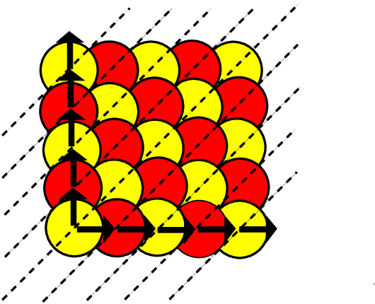
Refer to caption
Figure 13: The crystal for the NCDT chamber of 𝒪⁡(−2)⊕𝒪→ℙ1{\cal O}(-2)\oplus{\cal O}\rightarrow\mathbb{P}^{1}
Refer to caption
Figure 14: The crystal in the chamber (R>0,2<B<3)(R>0,2<B<3) copied from [27]
Refer to caption
Figure 15: The crystal in the chamber (R<0,4<B<5)(R<0,4<B<5) copied from [27]

Like the ℂ3{\mathds{C}}^{3} and resolved conifold cases, we also associate some vertex operators with the arrows (figure 16) in figure 13, 14, 15.

Refer to caption
Figure 16: Arrow diagrams for chamber nn of 𝒪⁡(−2)⊕𝒪→ℙ1{\cal O}(-2)\oplus{\cal O}\rightarrow\mathbb{P}^{1}. We use the red and yellow stones to distinguish those vertex operators which has (−Q)12(-Q)^{\frac{1}{2}} or (−Q)−12(-Q)^{-\frac{1}{2}} argument

First, let us see the NCDT chamber (R>0,0<B<1)(R>0,0<B<1). In this chamber the crystal diagram is shown in figure 13. According to the relation between the arrows and vertex operators shown in figure 16, we may find that

𝒵N​C​D​Tr​e​f\displaystyle\mathcal{Z}_{NCDT}^{ref} =\displaystyle= ⟨0|∏k=1∞Γ+​[q1k​(−Q)12]​Γ+​[q1k​(−Q)−12]​∏k=1∞Γ−​[q2k−1​(−Q)12]​Γ−​[q2k−1​(−Q)−12]|0⟩\displaystyle\langle 0|\prod_{k=1}^{\infty}\Gamma_{+}\left[q_{1}^{k}(-Q)^{\frac{1}{2}}\right]\Gamma_{+}\left[q_{1}^{k}(-Q)^{-\frac{1}{2}}\right]\prod_{k=1}^{\infty}\Gamma_{-}\left[q_{2}^{k-1}(-Q)^{\frac{1}{2}}\right]\Gamma_{-}\left[q_{2}^{k-1}(-Q)^{-\frac{1}{2}}\right]|0\rangle (6.57)
=\displaystyle= Mδ=12​(q1,q2)​∏i,j=1∞(1−q1i​q2j−1​Q)−1​∏i,j=1∞(1−q1i​q2j−1​Q−1)−1\displaystyle M_{\delta=1}^{2}(q_{1},q_{2})\prod_{i,j=1}^{\infty}(1-q_{1}^{i}q_{2}^{j-1}Q)^{-1}\prod_{i,j=1}^{\infty}(1-q_{1}^{i}q_{2}^{j-1}Q^{-1})^{-1}
=\displaystyle= Mδ=12​(q1,q2)​𝒵t​o​pr​e​f​(q1,q2,Q)​𝒵t​o​pr​e​f​(q1,q2,Q−1)|N​C​D​T​c​h​a​m​b​e​r\displaystyle M_{\delta=1}^{2}(q_{1},q_{2})\mathcal{Z}_{top}^{ref}(q_{1},q_{2},Q)\mathcal{Z}_{top}^{ref}(q_{1},q_{2},Q^{-1})|_{NCDTchamber}

We may also define A¯±​(x)\overline{A}_{\pm}(x) by

A¯+​(x):=Q^1−12​Γ+​(x)​Q^1​Γ+​(x)​Q^01​Q^112,\displaystyle\overline{A}_{+}(x):=\widehat{Q}_{1}^{-\frac{1}{2}}\Gamma_{+}(x)\widehat{Q}_{1}\Gamma_{+}(x)\widehat{Q}_{01}\widehat{Q}_{1}^{\frac{1}{2}}, (6.58)
A+​(x):=A¯+​(x)​(Q^1​Q^01)−1=Γ+​[(−Q)12​x]​Γ+​[(−Q)−12​x],\displaystyle A_{+}(x):=\overline{A}_{+}(x)(\widehat{Q}_{1}\widehat{Q}_{01})^{-1}=\Gamma_{+}\left[(-Q)^{\frac{1}{2}}x\right]\Gamma_{+}\left[(-Q)^{-\frac{1}{2}}x\right], (6.59)
A¯−​(x):=Q^1−12​Γ−​(x)​Q^1​Γ−​(x)​Q^02​Q^112,\displaystyle\overline{A}_{-}(x):=\widehat{Q}_{1}^{-\frac{1}{2}}\Gamma_{-}(x)\widehat{Q}_{1}\Gamma_{-}(x)\widehat{Q}_{02}\widehat{Q}_{1}^{\frac{1}{2}}, (6.60)
A−​(x):=A^−​(x)​(Q^1​Q^02)−1=Γ−​[(−Q)−12​x]​Γ−​[(−Q)12​x].\displaystyle A_{-}(x):=\widehat{A}_{-}(x)(\widehat{Q}_{1}\widehat{Q}_{02})^{-1}=\Gamma_{-}\left[(-Q)^{-\frac{1}{2}}x\right]\Gamma_{-}\left[(-Q)^{\frac{1}{2}}x\right]. (6.61)

where Q=−Q1,q1=Q01​Q1,q2=Q02​Q1Q=-Q_{1},q_{1}=Q_{01}Q_{1},q_{2}=Q_{02}Q_{1}. If we define⟨Ω+|\langle\Omega_{+}| and |Ω−⟩|\Omega_{-}\rangle by

⟨Ω+|\displaystyle\langle\Omega_{+}| :⁣=\displaystyle:= ⟨0|A¯+(1)⋯A¯+(1),\displaystyle\langle 0|\overline{A}_{+}(1)\cdots\overline{A}_{+}(1), (6.62)
|Ω−⟩\displaystyle|\Omega_{-}\rangle :⁣=\displaystyle:= A¯−(1)⋯A¯−(1)|0⟩,\displaystyle\overline{A}_{-}(1)\cdots\overline{A}_{-}(1)|0\rangle, (6.63)

then we can show that

𝒵N​C​D​Tr​e​f=⟨Ω+|Ω−⟩\mathcal{Z}_{NCDT}^{ref}=\langle\Omega_{+}|\Omega_{-}\rangle\\

For the chamber (R>0,0<n<B<n+1)(R>0,0<n<B<n+1), according to the correspondence between arrows and vertex operators (figure 16), we have the following formula:

𝒵B​P​Sr​e​f\displaystyle\mathcal{Z}_{BPS}^{ref} =\displaystyle= ⟨0|∏k=1∞Γ+[q1k(−Q)12]Γ+[q1k+n(−Q)−12]⋅\displaystyle\langle 0|\prod_{k=1}^{\infty}\Gamma_{+}\left[q_{1}^{k}(-Q)^{\frac{1}{2}}\right]\Gamma_{+}\left[q_{1}^{k+n}(-Q)^{-\frac{1}{2}}\right]\cdot (6.64)
Γ−[(−Q)−12]Γ+[q1n(−Q)−12]Γ−[q2(−Q)−12]Γ+[q1n−1(−Q)−12]⋯\displaystyle\Gamma_{-}\left[(-Q)^{-\frac{1}{2}}\right]\Gamma_{+}\left[q_{1}^{n}(-Q)^{-\frac{1}{2}}\right]\Gamma_{-}\left[q_{2}(-Q)^{-\frac{1}{2}}\right]\Gamma_{+}\left[q_{1}^{n-1}(-Q)^{-\frac{1}{2}}\right]\cdots
Γ−​[q2n−1​(−Q)−12]​Γ+​[q1​(−Q)−12]⋅∏k=1∞Γ−​[q2k+n−1​(−Q)−12]​Γ−​[q2k−1​(−Q)12]​|0⟩\displaystyle\Gamma_{-}\left[q_{2}^{n-1}(-Q)^{-\frac{1}{2}}\right]\Gamma_{+}\left[q_{1}(-Q)^{-\frac{1}{2}}\right]\cdot\prod_{k=1}^{\infty}\Gamma_{-}\left[q_{2}^{k+n-1}(-Q)^{-\frac{1}{2}}\right]\Gamma_{-}\left[q_{2}^{k-1}(-Q)^{\frac{1}{2}}\right]|0\rangle
=\displaystyle= Mδ=12​(q1,q2)​∏i,j=1∞(1−q1i​q2j−1​Q)−1​∏i+j>n+1(1−q1i​q2j−1​Q−1)−1\displaystyle M_{\delta=1}^{2}(q_{1},q_{2})\prod_{i,j=1}^{\infty}(1-q_{1}^{i}q_{2}^{j-1}Q)^{-1}\prod_{i+j>n+1}(1-q_{1}^{i}q_{2}^{j-1}Q^{-1})^{-1}
=\displaystyle= Mδ=12(q1,q2)𝒵t​o​pr​e​f(q1,q2,Q)𝒵t​o​pr​e​f(q1,q2,Q−1)|(R>0,0<n<B<n+1)\displaystyle M_{\delta=1}^{2}(q_{1},q_{2})\mathcal{Z}_{top}^{ref}(q_{1},q_{2},Q)\mathcal{Z}_{top}^{ref}(q_{1},q_{2},Q^{-1})|_{(R>0,0<n<B<n+1)}

Similarly for the chamber (R<0,0<B<1)(R<0,0<B<1),we also have

𝒵B​P​Sr​e​f=⟨0|0⟩=1,\mathcal{Z}_{BPS}^{ref}=\langle 0|0\rangle=1, (6.65)

and for the chamber R<0,1≤n<B<n+1R<0,1\leq n<B<n+1,we also have

𝒵B​P​Sr​e​f\displaystyle\mathcal{Z}_{BPS}^{ref} =\displaystyle= ⟨0|Γ+[q1(−Q)−12]Γ−[q2n−1(−Q)−12]⋯Γ+[q1n(−Q)−12]Γ−[(−Q)−12]|0⟩\displaystyle\langle 0|\Gamma_{+}\left[q_{1}(-Q)^{-\frac{1}{2}}\right]\Gamma_{-}\left[q_{2}^{n-1}(-Q)^{-\frac{1}{2}}\right]\cdots\Gamma_{+}\left[q_{1}^{n}(-Q)^{-\frac{1}{2}}\right]\Gamma_{-}\left[(-Q)^{-\frac{1}{2}}\right]|0\rangle (6.66)
=\displaystyle= ∏i,j=1n(1−q1i​q2j−1​Q−1)−1.\displaystyle\prod_{i,j=1}^{n}(1-q_{1}^{i}q_{2}^{j-1}Q^{-1})^{-1}.

7 Discussion

In this paper, we first use the M-theory to propose the so-called refined reminiscence of the OSV formula connecting the refined BPS states partition function with the refined topological string partition function. Secondly, we produce the wall-crossing formulas of the refined BPS states partition function by employing the vertex operators in 2-dimensional free fermions. Like in [10], here we also require that the Calabi-Yau threefold XX does NOT contain any compact four cycles.

For the the refined reminiscence of the OSV formula we proposed in section 2, in the equation (2.17) there is a factor ℳ⁡(q1,q2)\mathcal{M}(q_{1},q_{2}), which is related to the refined MacMahon function, appearing in the refined topological string partition function. It should be related to the D0-branes bounded to the single D6-brane. We notice that in [16], the authors investigated the motivic degree zero of Donaldson-Thomas generating function on ℂ3{\mathds{C}}^{3} and some other smooth projective threefolds. In the appendix of their paper, they explained how to relate the motivic degree zero of Donaldson-Thomas generating function on ℂ3{\mathds{C}}^{3} to Okounkov et al.’s refined generating function in counting plane partitions in [17]. For example, the motivic degree zero of Donaldson-Thomas generating function on ℂ3{\mathds{C}}^{3} is related to the refined MacMahon function 55 5 Here we use the convention δ2\frac{\delta}{2} in equation (2.19) as the definition of the refined MacMahon function Mδ​(q1,q2)M_{\delta}(q_{1},q_{2}) which is a little bit different with the definition in [16]. Mδ=−3​(q1,q2)M_{\delta=-3}(q_{1},q_{2}) appearing in [17]. For other toric CYs, the theorem 3.7 in [16] shows how to refine the MacMahon function. The puzzle is that the refined MacMahon functions appearing in [16] are different with the refined MacMahon functions proposed in this paper. It would be very interesting to see how to reproduce the refined MacMahon functions appearing in [16] by using the method proposed in this paper. We believe that well-understanding on [16] will shed some light on this direction.

In this paper, we only investigate the simplest three Calabi-Yau threefolds ℂ3,𝒪⁡(−1)⊕𝒪⁡(−1)→ℙ1{\mathds{C}}^{3},\mathcal{O}(-1)\oplus\mathcal{O}(-1)\rightarrow\mathbb{P}^{1}, and 𝒪⁡(−2)⊕𝒪→ℙ1\mathcal{O}(-2)\oplus\mathcal{O}\rightarrow\mathbb{P}^{1}. Then we may ask for other more complicated threefolds, especially those coming from the strip [30], how do we use the vertex operator techniques to write down the wall-crossing formulas of the refined BPS partition functions for them? This work is in progress.

Further, in [12], the authors investigated the refined wall-crossing for the resolved conifold case by using the dimer model. We believe that using dimer model we can also get the refined wall-crossing formulas for the 𝒪⁡(−2)⊕𝒪→ℙ1\mathcal{O}(-2)\oplus\mathcal{O}\rightarrow\mathbb{P}^{1} and other cases. We are working in this direction.

Finally, in [31, 32], the authors investigated the relation between the matrix models and the wall-crossing. For the refined wall-crossing case, it is not difficult to find that one can indeed use matrix model to reproduce the refined NCDT partition function. It would be interesting to use the matrix model to reproduce the refined wall-crossing formula; it would also be interesting to see the details of this kind of matrix model, e.g. spectral curve, etc. This work is under consideration.

Acknowledgements

We would like to thank Prof. Balázs Szendrői and Dr. Masahito Yamazaki for the valuable comments.

H. Liu thanks Yunfeng Jiang for the valuable discussion at the final stage of this project and also thanks the hospitality and inspiring atmosphere of the 8th Simons Workshop on Mathematics and Physics and the hospitality of the theoretical physics group of Imperial College while preparing this paper. H. Liu also appreciates Prof. Jack Gegenberg for his support. The research of H. Liu is partially supported by the “Pam and John Little Overseas Scholarship” in the University of New Brunswick, Canada.

J. Yang thanks the wonderful working atmosphere provided by SISSA. The experience and the friendship are most valuable for her.

References

  • [1] H. Ooguri, A. Strominger, and C. Vafa, Black hole attractors and the topological string, Phys. Rev. D70 (2004) 106007, [hep-th/0405146].
  • [2] J. A. Harvey and G. W. Moore, On the algebras of bps states, Commun. Math. Phys. 197 (1998) 489–519, [hep-th/9609017].
  • [3] R. Minasian and G. W. Moore, K-theory and ramond-ramond charge, JHEP 11 (1997) 002, [hep-th/9710230].
  • [4] F. Denef and G. W. Moore, Split states, entropy enigmas, holes and halos, hep-th/0702146.
  • [5] E. Diaconescu and G. W. Moore, Crossing the wall: Branes vs. bundles, arXiv:0706.3193.
  • [6] A. Dabholkar, F. Denef, G. W. Moore, and B. Pioline, Exact and asymptotic degeneracies of small black holes, JHEP 08 (2005) 021, [hep-th/0502157].
  • [7] B. Szendroi, Non-commutative donaldson-thomas theory and the conifold, Geom.Topol. 12:1171-1202,2008 (May, 2007) [arXiv:0705.3419].
  • [8] D. Gaiotto, G. W. Moore, and A. Neitzke, Four-dimensional wall-crossing via three-dimensional field theory, Commun. Math. Phys. 299 (2010) 163–224, [arXiv:0807.4723].
  • [9] B. Young and J. Bryan, Generating functions for colored 3d young diagrams and the donaldson-thomas invariants of orbifolds, arXiv:0802.3948.
  • [10] M. Aganagic, H. Ooguri, C. Vafa, and M. Yamazaki, Wall crossing and m-theory, arXiv:0908.1194.
  • [11] M. Aganagic and K. Schaeffer, Wall crossing, quivers and crystals, arXiv:1006.2113.
  • [12] T. Dimofte and S. Gukov, Refined, motivic, and quantum, Lett. Math. Phys. 91 (2010) 1, [arXiv:0904.1420].
  • [13] M. Kontsevich and Y. Soibelman, Stability structures, motivic donaldson-thomas invariants and cluster transformations, arXiv:0811.2435.
  • [14] T. J. Hollowood, A. Iqbal, and C. Vafa, Matrix models, geometric engineering and elliptic genera, JHEP 03 (2008) 069, [hep-th/0310272].
  • [15] A. Iqbal, C. Kozcaz, and C. Vafa, The refined topological vertex, JHEP 10 (2009) 069, [hep-th/0701156].
  • [16] K. Behrend, J. Bryan, and B. Szendroi, Motivic degree zero donaldson-thomas invariants, arXiv:0909.5088.
  • [17] A. Okounkov and N. Reshetikhin, Random skew plane partitions and the pearcey process, math/0503508.
  • [18] M. Jimbo and T. Miwa, Solitons and infinite dimensional lie algebra, Publ. RIMS, Kyoto Univ. 19 (1983) 943–1001.
  • [19] I. G. Macdonald, Symmetric Functions and Hall Polynomials. Oxford Mathematical Monographs. Oxford University Press, 2 ed., 1999.
  • [20] A. Okounkov, N. Reshetikhin, and C. Vafa, Quantum calabi-yau and classical crystals, hep-th/0309208.
  • [21] A. Iqbal, N. Nekrasov, A. Okounkov, and C. Vafa, Quantum foam and topological strings, JHEP 04 (2008) 011, [hep-th/0312022].
  • [22] P. Sulkowski, Calabi-yau crystals in topological string theory, arXiv:0712.2173.
  • [23] R. Dijkgraaf, D. Orlando, and S. Reffert, Dimer models, free fermions and super quantum mechanics, arXiv:0705.1645.
  • [24] R. Dijkgraaf, L. Hollands, P. Sulkowski, and C. Vafa, Supersymmetric gauge theories, intersecting branes and free fermions, JHEP 02 (2008) 106, [arXiv:0709.4446].
  • [25] A. Okounkov and N. Reshetikhin, Correlation function of schur process with application to local geometry of a random 3-dimensional young diagram, math/0107056.
  • [26] G. E. Andrews, Generalized Frobenius partitions. No. 301 in Memoirs of the AMS. 1984.
  • [27] P. Sulkowski, Wall-crossing, free fermions and crystal melting, arXiv:0910.5485.
  • [28] B. Young, Computing a pyramid partition generating function with dimer shuffling, arXiv:0709.3079.
  • [29] M. Taki, Flop invariance of refined topological vertex and link homologies, arXiv:0805.0336.
  • [30] A. Iqbal and A.-K. Kashani-Poor, The vertex on a strip, Adv. Theor. Math. Phys. 10 (2006) 317–343, [hep-th/0410174].
  • [31] H. Ooguri, P. Sulkowski, and M. Yamazaki, Wall crossing as seen by matrix models, arXiv:1005.1293.
  • [32] R. J. Szabo and M. Tierz, Matrix models and stochastic growth in donaldson-thomas theory, arXiv:1005.5643.