跳到论文正文
W Papers独立论文阅读器 arXiv:1010.0232 论文正文 计算阅读时间 · 0%
引用这篇论文根据当前论文元数据生成,正式投稿前建议核对。


License: arXiv.org perpetual non-exclusive license
arXiv:1010.0232v2 [math.CO] 13 Oct 2011

Eigenvectors for a random walk on a hyperplane arrangementThanks: 1Partially supported by NSERC of Canada and the Swiss National Science Foundation

Graham Denham1 Address: Department of Mathematics, University of Western Ontario
London, ON N6A 5B7, Canada
URL: http://www.math.uwo.ca/˜gdenham
Date: August 24, 2026
Abstract.

We find explicit eigenvectors for the transition matrix of the Bidegare-Hanlon-Rockmore random walk, from [1]. This is accomplished by using Brown and Diaconis’ analysis in [3] of the stationary distribution, together with some combinatorics of functions on the face lattice of a hyperplane arrangement, due to Gel′fand and Varchenko [10].

Key words and phrases: 
hyperplane arrangement, random walk, oriented matroid
2000 Mathematics Subject Classification
Primary 52C35. Secondary 60J10.

1. Introduction

In 1999, Bidegare, Hanlon and Rockmore [1] introduced a simultaneous generalization of several well-studied discrete Markov chains. Let 𝒜{\mathcal{A}} be an arrangement of nn linear hyperplanes in W=ℝℓW={\mathbb{R}}^{\ell}, and let 𝒞{\mathcal{C}} denote the set of chambers: i.e., the connected components of the complement of 𝒜{\mathcal{A}} in WW. They construct a random walk on 𝒞{\mathcal{C}}, which we will follow [3] in calling the BHR random walk, by means of the face product, defined below. By choosing the hyperplane arrangement suitably, one obtains as special cases the Tsetlin library (“move-to-front rule”), Ehrenfests’ urn, and various card-shuffling models [1, 3].

A key insight in this construction and main result of [1] is that the eigenvalues of the transition matrix can be expressed simply in terms of the combinatorics of the arrangement 𝒜{\mathcal{A}}. This is useful for bounding the rate of convergence to the stationary distribution: Brown and Diaconis make this analysis in [3], show that the transition matrix is diagonalizable, and give an explicit description of the random walk’s stationary distribution.

Subsequently Brown [2] generalized the BHR random walk to the setting of certain semigroup algebras, showing in particular that the diagonalization result held there as well. He describes projection operators onto each eigenspace, which in principle provides a description of the eigenvectors of the random walk’s transition matrix. However, the general expression is necessarily somewhat complicated.

The purpose of this paper, then, is to provide a relatively straightforward description of the original BHR random walk’s eigenvectors. It turns out that the combinatorial Heaviside functions of Gel′fand and Varchenko [10] behave well with respect to the face product and the BHR random walk, so we highlight their role in this problem. Using the description of the stationary distribution from [3], the main result here, Theorem 3.6, describes a spanning set for each eigenspace in terms of flags in the intersection lattice.

2. Background and notation

2.1. The face algebra

Let 𝒜{\mathcal{A}} be an arrangement of nn hyperplanes in ℝℓ{\mathbb{R}}^{\ell}. We will assume throughout that 𝒜{\mathcal{A}} is central and essential: that is, the intersection of the hyperplanes 𝒜{\mathcal{A}} equals the origin in ℝℓ{\mathbb{R}}^{\ell}. We will follow the notational conventions of the standard reference for hyperplane arrangements, [6]. In particular, let L⁡(𝒜)L({\mathcal{A}}) denote the lattice of intersections, ordered by reverse inclusion, and ℱ=ℱ⁡(𝒜){\mathcal{F}}={\mathcal{F}}({\mathcal{A}}) the face semilattice, also ordered by reverse inclusion. For 0≤p≤ℓ0\leq p\leq\ell, let Lp​(𝒜)L_{p}({\mathcal{A}}) and ℱp​(𝒜){\mathcal{F}}_{p}({\mathcal{A}}) denote the subspaces and faces, respectively, of codimension pp. In particular, the set of chambers 𝒞=𝒞⁡(𝒜)=ℱ0​(𝒜){\mathcal{C}}={\mathcal{C}}({\mathcal{A}})={\mathcal{F}}_{0}({\mathcal{A}}).

For a face F∈ℱF\in{\mathcal{F}}, let |F|{\lvert F\rvert} denote the smallest subspace in L⁡(𝒜)L({\mathcal{A}}) containing FF. Recall that 𝒜X{\mathcal{A}}^{X} denotes the arrangement in XX of hyperplanes {H∩X:H∈𝒜,X⊈H}{\left\{H\cap X\colon H\in{\mathcal{A}},X\not\subseteq H\right\}}, whenever X∈L⁡(𝒜)X\in L({\mathcal{A}}), and 𝒜X{\mathcal{A}}_{X} denotes the subarrangement {H∈𝒜:X⊆H}{\left\{H\in{\mathcal{A}}\colon X\subseteq H\right\}}. We will identify faces (and chambers) of 𝒜X{\mathcal{A}}^{X} with faces F∈ℱ⁡(𝒜)F\in{\mathcal{F}}({\mathcal{A}}) for which |F|≥X{\lvert F\rvert}\geq X (and |F|=X{\lvert F\rvert}=X, respectively):

(2.1) ℱ⁡(𝒜X)≅{F∈ℱ⁡(𝒜):|F|≥X}.{\mathcal{F}}({\mathcal{A}}^{X})\cong{\left\{F\in{\mathcal{F}}({\mathcal{A}})\colon{\lvert F\rvert}\geq X\right\}}.

For hyperplanes H∈𝒜H\in{\mathcal{A}}, let FHF_{H} be 0,±10,\pm 1 depending on whether FF is contained in HH, on the positive side, or the negative side, respectively. We will abbreviate the values of FHF_{H} with 0,+,−0,{\mathchar 43},{\mathchar 512}. A face FF is uniquely determined by the sign sequence (FH)H∈𝒜(F_{H})_{H\in{\mathcal{A}}}.

We recall the face product of two faces FF and GG can be described by its sign sequence:

(2.2) (F​G)H={FHif FH≠0;GHotherwise.(FG)_{H}=\begin{cases}F_{H}&\text{if $F_{H}\neq 0$;}\\ G_{H}&\text{otherwise.}\end{cases}

From the definition, F​F=FFF=F for any FF, and F​G​F=F​GFGF=FG for any faces F,GF,G (the “deletion property”: see [2].)

For a fixed arrangement 𝒜{\mathcal{A}}, let A=R⁡[ℱ]A=R[{\mathcal{F}}] denote its face algebra, introduced in [3]. Additively, AA is the free RR-module on ℱ{\mathcal{F}}, and multiplication is given by linearly extending the face product. Following [3], let V⁡(𝒜)V({\mathcal{A}}) denote the free RR-module on 𝒞⁡(𝒜){\mathcal{C}}({\mathcal{A}}): then the face product makes V⁡(𝒜)V({\mathcal{A}}) a left AA-module. More generally, following [3, Section 5C], we can make V⁡(𝒜X)V({\mathcal{A}}^{X}) a left AA-module for any X∈L⁡(𝒜)X\in L({\mathcal{A}}): for F∈ℱF\in{\mathcal{F}} and G∈𝒞⁡(𝒜X)G\in{\mathcal{C}}({\mathcal{A}}^{X}), set

(2.3) F​G={F​Gif |F|≥X;0otherwise.FG=\begin{cases}FG&\text{if ${\lvert F\rvert}\geq X$;}\\ 0&\text{otherwise.}\end{cases}

2.2. The zonotope of a real arrangement

Refer to caption
Figure 1. Zonotope for f1=xf_{1}=x, f2=yf_{2}=y, f3=x−yf_{3}=x-y.

As Brown and Diaconis [3] observe, it is useful in this setting to consider the zonotope of a real arrangement. Let fHf_{H} denote a linear equation defining the hyperplane HH, for each H∈𝒜H\in{\mathcal{A}}. The zonotope Z𝒜Z_{\mathcal{A}} is, by definition, the Minkowski sum of intervals,

Z𝒜=∑H∈𝒜[−fH,fH].Z_{\mathcal{A}}=\sum_{H\in{\mathcal{A}}}[-f_{H},f_{H}].

This is a polytope in W∗W^{*}: we refer to [12] for details. Its most relevant feature here is that the face poset of Z𝒜Z_{\mathcal{A}} (ordered by inclusion) is isomorphic to ℱ⁡(𝒜){\mathcal{F}}({\mathcal{A}}): the isomorphism arises by identifying the outer normal fan of the zonotope with the arrangement. If FF is a face of 𝒜{\mathcal{A}}, then, let F^\hat{F} denote the corresponding face of the zonotope. Each face F^\hat{F} is an affine translate of a zonotope of a closed subarrangement: for F∈ℱF\in{\mathcal{F}}, let X=|F|X={\lvert F\rvert} and vF=∑H∈𝒜(FH)​fHv_{F}=\sum_{H\in{\mathcal{A}}}(F_{H})f_{H}. Then F^=vF+Z𝒜X\hat{F}=v_{F}+Z_{{\mathcal{A}}_{X}}: see, for example, discussion in [5].

For the sake of intuition, we indicate one way to visualize the face product in the zonotope world.

Definition 2.3.

Suppose PP is a polytope in W∗W^{*} and v∈W∗v\in W^{*} is nonzero. Define a map rP,v:P+[−v,v]→P+vr_{P,v}\colon P+[-v,v]\to P+v as follows. If p∈P+[−v,v]p\in P+[-v,v], let λ\lambda be maximal for which p=x+λ​vp=x+\lambda v, where x∈Px\in P and λ≤1\lambda\leq 1. Set rP,v​(p)=x+vr_{P,v}(p)=x+v. Clearly rP,vr_{P,v} is piecewise-linear and fixes P+vP+v pointwise.

Proposition 2.4.

For each face FF of 𝒜{\mathcal{A}}, there is a piecewise-linear retract pFp_{F} of Z𝒜Z_{\mathcal{A}} onto F^\hat{F}, with pF​(G^)=F​G^p_{F}(\hat{G})=\widehat{FG}, for all G∈ℱ⁡(𝒜)G\in{\mathcal{F}}({\mathcal{A}}).

Proof.

We will write pFp_{F} as the composition of the retracts from Definition 2.3, one for each hyperplane of 𝒜{\mathcal{A}} not containing FF.

Again, let X=|F|X={\lvert F\rvert}. Let S1={fH:FH=0}S_{1}={\left\{f_{H}\colon F_{H}=0\right\}} and S2={(FH)​fH:FH≠0}S_{2}={\left\{(F_{H})f_{H}\colon F_{H}\neq 0\right\}}. Then

Z𝒜\displaystyle Z_{\mathcal{A}} =\displaystyle= ∑v∈S1[−v,v]+∑v∈S2[−v,v]\displaystyle\sum_{v\in S_{1}}[-v,v]+\sum_{v\in S_{2}}[-v,v]
=\displaystyle= Z𝒜X+∑v∈S2[−v,v],\displaystyle Z_{{\mathcal{A}}_{X}}+\sum_{v\in S_{2}}[-v,v],

and vF=∑v∈S2vv_{F}=\sum_{v\in S_{2}}v. Put the elements of S2S_{2} in any order, writing S2={v1,v2,…,vk}S_{2}={\left\{v_{1},v_{2},\ldots,v_{k}\right\}}. Let P0=Z𝒜X+vFP_{0}=Z_{{\mathcal{A}}_{X}}+v_{F}, and let Pi=Pi−1+[−2​vi,0]P_{i}=P_{i-1}+[-2v_{i},0] for 1≤i≤k1\leq i\leq k. Then

F^=P0⊆P1⊆⋯⊆Pk=Z𝒜,\hat{F}=P_{0}\subseteq P_{1}\subseteq\cdots\subseteq P_{k}=Z_{\mathcal{A}},

and the following composite collapses along the vectors in S2S_{2}, one at a time:

pF=rP0−v1,v1∘rP1−v2,v2∘⋯∘rPk−1−vk,vk:Z𝒜→F^.p_{F}=r_{P_{0}-v_{1},v_{1}}\circ r_{P_{1}-v_{2},v_{2}}\circ\cdots\circ r_{P_{k-1}-v_{k},v_{k}}\colon Z_{\mathcal{A}}\to\hat{F}.

By construction, this is a piecewise-linear retract onto F^\hat{F}.

To see that pF​(G^)=F​G^p_{F}(\hat{G})=\widehat{FG} for any face GG, let S∈(±1)𝒜S\in(\pm 1)^{\mathcal{A}} be an arbitrary sequence of nonzero signs, and define vS=∑H∈𝒜SH​fHv_{S}=\sum_{H\in{\mathcal{A}}}S_{H}f_{H}. Then rPi−1−vi,vi​(vS)=vS′,r_{P_{i-1}-v_{i},v_{i}}(v_{S})=v_{S^{\prime}}, where

(S′)H={SHif fH≠±vi;cif fH=c​vi.(S^{\prime})_{H}=\begin{cases}S_{H}&\text{if $f_{H}\neq\pm v_{i}$;}\\ c&\text{if $f_{H}=cv_{i}$.}\end{cases}

It follows that pF​(C^)=F​C^p_{F}(\hat{C})=\widehat{FC} for chambers C∈𝒞⁡(𝒜)C\in{\mathcal{C}}({\mathcal{A}}). By writing an arbitrary face G^\hat{G} as the convex hull of the vertices C^\hat{C} for which C≤GC\leq G, one then obtains pF​(G^)=F​G^p_{F}(\hat{G})=\widehat{FG} for all GG. ∎

Note that the map pFp_{F} is not uniquely defined, and depends on a choice of order. See Figure 2 for examples.

Refer to caption
(a) pFp_{F} with F=−0++F={\mathchar 512}0{\mathchar 43}{\mathchar 43}
Refer to caption
(b) pFp_{F} with F=00++0F=00{\mathchar 43}{\mathchar 43}0
Figure 2. Retracts onto faces of zonotopes of dimension 22 and 33

2.5. The BHR random walk

Let 𝒜{\mathcal{A}} be an arrangement, and w:ℱ→ℝw\colon{\mathcal{F}}\to{\mathbb{R}} a discrete probability distribution on the faces of 𝒜{\mathcal{A}}. The random walk introduced in [1] is a random walk on chambers, taking C∈𝒞C\in{\mathcal{C}} to F​CFC with probability wFw_{F}. Its transition matrix K=K𝒜K=K_{\mathcal{A}} can be regarded as a linear endomorphism of the vector space with basis 𝒞{\mathcal{C}}, given by

(2.4) K⁡(C)=∑F∈ℱwF​F​C.K(C)=\sum_{F\in{\mathcal{F}}}w_{F}FC.

An eigenvector of KK with eigenvalue 11 gives a stationary distribution for the random walk. Brown and Diaconis [3, Theorem 2] find that, with an assumption of nondegeneracy, the eigenspace is 11-dimensional, which is to say the stationary distribution is unique. In this case, it is given by sampling faces without replacement: explicitly, one sums over all permutations of the faces to obtain

(2.5) πC=∑σ∈SN:C=Fσ⁡(1)⋯Fσ⁡(N)∏1≤p≤NwFσ⁡(p)1−∑i<pwFσ⁡(i),\pi_{C}=\sum_{\begin{subarray}{c}\sigma\in S_{N}\colon\\ C=F_{\sigma(1)}\cdots F_{\sigma(N)}\end{subarray}}\prod_{1\leq p\leq N}\frac{w_{F_{\sigma(p)}}}{1-\sum_{i<p}w_{F_{\sigma(i)}}},

where N=|ℱ|N={\lvert{\mathcal{F}}\rvert}, the number of faces. The complete list of eigenvalues is given as follows, where μ\mu denotes the Möbius function of L⁡(𝒜)L({\mathcal{A}}). For each X∈L⁡(𝒜)X\in L({\mathcal{A}}), let

(2.6) λX=∑F:|F|≥XwF.\lambda_{X}=\sum_{F\colon{\lvert F\rvert}\geq X}w_{F}.

(Equivalently, λX=∑F∈ℱ⁡(𝒜X)wF\lambda_{X}=\sum_{F\in{\mathcal{F}}({\mathcal{A}}^{X})}w_{F}, by (2.1).)

Theorem 2.6 ([1, 3]).

For each X∈Lp​(𝒜)X\in L_{p}({\mathcal{A}}), for 0≤p≤ℓ0\leq p\leq\ell, the matrix KK has an eigenspace of multiplicity (−1)p​μ​(W,X)(-1)^{p}\mu(W,X) with eigenvalue λX\lambda_{X}.

The main result here is a corresponding basis of eigenvectors for each eigenvalue, Theorem 3.6. For this, it is convenient to regard the distribution weights wFw_{F} as indeterminates as in [2], diagonalize, and then specialize afterwards: let R=ℝ(wF:F∈ℱ)R={\mathbb{R}}(w_{F}\colon F\in{\mathcal{F}}), the fraction field of polynomials in the variables wFw_{F}. In doing so, we relax the condition that the weights sum to 11, so (2.5) needs to be adjusted accordingly. Let q∈V⁡(𝒜)q\in V({\mathcal{A}}) be the vector whose coordinate on chamber CC is given by

(2.7) qC=∑σ∈SN:C=Fσ⁡(1)⋯Fσ⁡(N)∏p=1N(∑i=pNwFσ⁡(i))−1.q_{C}=\sum_{\begin{subarray}{c}\sigma\in S_{N}\colon\\ C=F_{\sigma(1)}\cdots F_{\sigma(N)}\end{subarray}}\prod_{p=1}^{N}\big(\sum_{i=p}^{N}w_{F_{\sigma(i)}}\big)^{-1}.
Lemma 2.7.

For any arrangement 𝒜{\mathcal{A}}, the vector qq is a λW\lambda_{W}-eigenvector of KK.

Proof.

We provide a direct calculation in lieu of adapting the corresponding result from [3]. For succinctness, let

f⁡(x1,…,xN)=∏i=1N(∑i=pNxi)−1f(x_{1},\ldots,x_{N})=\prod_{i=1}^{N}\big(\sum_{i=p}^{N}x_{i}\big)^{-1}

for any choice of xix_{i}’s, and abbreviate f⁡(σ):=f⁡(wFσ⁡(1),…,wFσ⁡(N))f(\sigma):=f(w_{F_{\sigma(1)}},\ldots,w_{F_{\sigma(N)}}) for any permutation of the faces σ∈SN\sigma\in S_{N}. By clearing denominators, one may verify the identity

f⁡(x1,…,xN)+\displaystyle f(x_{1},\ldots,x_{N})+ f⁡(x2,x1,x3,…,xN)+⋯\displaystyle f(x_{2},x_{1},x_{3},\ldots,x_{N})+\cdots
(2.8) +f⁡(x2,…,xN,x1)=f⁡(x1,…,xN)⋅(∑i=1Nxi)/x1.\displaystyle+f(x_{2},\ldots,x_{N},x_{1})=f(x_{1},\ldots,x_{N})\cdot\big(\sum_{i=1}^{N}x_{i}\big)/x_{1}.

For 1≤i≤N1\leq i\leq N, let σi\sigma_{i} denote the ii-cycle (1,2,…,i)∈SN(1,2,\ldots,i)\in S_{N}. Then (2.8) states that

(2.9) ∑i=1Nf⁡(σ​σi−1)=(λW/x1)​f​(σ),\sum_{i=1}^{N}f(\sigma\sigma_{i}^{-1})=(\lambda_{W}/x_{1})f(\sigma),

since λW=∑i=1NwFi\lambda_{W}=\sum_{i=1}^{N}w_{F_{i}}.

Now K​q=∑F∈ℱwF​qC​(F​C)Kq=\sum_{F\in{\mathcal{F}}}w_{F}q_{C}(FC). For each C∈𝒞C\in{\mathcal{C}}, we compute:

(K​q)C\displaystyle(Kq)_{C} =\displaystyle= ∑F,C′:C=F​C′wFqC′\displaystyle\sum_{F,C^{\prime}\colon C=FC^{\prime}}w_{F}q_{C^{\prime}}
=\displaystyle= ∑F∈ℱ,σ∈SN:C=FFσ⁡(1)⋯Fσ⁡(N)wFf(σ)\displaystyle\sum_{\begin{subarray}{c}F\in{\mathcal{F}},\;\sigma\in S_{N}\colon\\ C=FF_{\sigma(1)}\cdots F_{\sigma(N)}\end{subarray}}w_{F}f(\sigma)
=\displaystyle= ∑σ∈SN:C=Fσ⁡(1)⋯Fσ⁡(N)∑i=1NwFσ⁡(1)f(σσi−1), by the deletion property, §2.1,\displaystyle\sum_{\begin{subarray}{c}\sigma\in S_{N}\colon\\ C=F_{\sigma(1)}\cdots F_{\sigma(N)}\end{subarray}}\sum_{i=1}^{N}w_{F_{\sigma(1)}}f(\sigma\sigma_{i}^{-1}),\text{~by the deletion property, \lx@sectionsign\ref{ss:face},}
=\displaystyle= λW​qC, by (2.9).\displaystyle\lambda_{W}q_{C},\text{~by \eqref{eq:identity2}.}

∎

Remark 2.8.

As written, the weights {wF}{\left\{w_{F}\right\}} in (2.7) only admit specializations to nonzero real numbers. One may clear denominators to obtain a general polynomial expression for an eigenvector, however this is clumsy to write in general.

2.9. Combinatorial Heaviside functions

We will recover Theorem 2.6, together with eigenvectors, by exploiting some fundamental structural results of Varchenko and Gel′fand [10], which we briefly describe here. For more details, see [4].

The Varchenko-Gel′fand ring of 𝒜{\mathcal{A}} is defined additively to be simply the space of linear functionals on chambers, V∗V^{*}. The ring structure is given by coordinatewise multiplication. The interest lies in the choice of generators: for each hyperplane H∈𝒜H\in{\mathcal{A}}, let xH∈V∗x_{H}\in V^{*} be the function defined by

xH​(C)={1if C is on the positive side of H;0otherwise.x_{H}(C)=\begin{cases}1&\text{if $C$ is on the positive side of $H$;}\\ 0&\text{otherwise.}\end{cases}

For a set of hyperplanes I⊆𝒜I\subseteq{\mathcal{A}}, let xIx_{I} be the monomial xI=∏H∈IxHx_{I}=\prod_{H\in I}x_{H}. (Since each xHx_{H} is idempotent, we only need to consider square-free monomials.) Let 1∈V∗1\in V^{*} be the function given by 1​(C)=11(C)=1 for all chambers C∈𝒞C\in{\mathcal{C}}.

In [10], it is shown that the Varchenko-Gel′fand ring admits a presentation much like the Orlik-Solomon algebra, with generators xHx_{H} and certain combinatorial relations: see [7] for an interpretation that compares the two. Unlike the Orlik-Solomon algebra, however, the relations amongst the generators are inhomogeneous, so it is useful to define a degree filtration by letting

PpV∗={f∈V∗:f can be written as a polynomial in xH’s of degree at most p.}P_{p}V^{*}={\left\{f\in V^{*}\colon\text{$f$ can be written as a polynomial in $x_{H}$'s of degree at most $p$.}\right\}}

By [10, Theorem 1],

V∗=PℓV∗⊇Pℓ−1V∗⊇⋯P0V∗⊋0,V^{*}=P_{\ell}V^{*}\supseteq P_{\ell-1}V^{*}\supseteq\cdots P_{0}V^{*}\supsetneq 0,

with the function 11 spanning P0P_{0}. The filtration is “natural” in the sense that, if ℬ{\mathcal{B}} is a subarrangement of 𝒜{\mathcal{A}}, containment gives a map of chambers 𝒞⁡(𝒜)→𝒞⁡(ℬ){\mathcal{C}}({\mathcal{A}})\to{\mathcal{C}}({\mathcal{B}}). This induces a map V​(ℬ)∗→V​(𝒜)∗V({\mathcal{B}})^{*}\to V({\mathcal{A}})^{*}, which is easily seen to preserve the degree filtration.

Now let grp⁡V∗=Pp​V∗/Pp−1​V∗\gr_{p}V^{*}=P_{p}V^{*}/P_{p-1}V^{*}, for 0≤p≤ℓ0\leq p\leq\ell. Let bp=(−1)p​∑X∈Lp​(𝒜)μ⁡(W,X)b_{p}=(-1)^{p}\sum_{X\in L_{p}({\mathcal{A}})}\mu(W,X), the ppth Betti number of the arrangement. Then the degree filtration satisfies an analogue of Brieskorn’s Lemma for arrangements:

Theorem 2.10 (Theorem 3, Corollaries 2,3 in [10]).

For 0≤p≤ℓ0\leq p\leq\ell, grp⁡V∗\gr_{p}V^{*} is a free module, of rank equal to bp​(𝒜)b_{p}({\mathcal{A}}). More precisely, there are isomorphisms

(2.10) grp⁡V​(𝒜)∗≅⨁X∈Lp​(𝒜)grp⁡V​(𝒜X)∗.\gr_{p}V({\mathcal{A}})^{*}\cong\bigoplus_{X\in L_{p}({\mathcal{A}})}\gr_{p}V({\mathcal{A}}_{X})^{*}.

induced by the inclusion of the arrangement 𝒜X{\mathcal{A}}_{X} into 𝒜{\mathcal{A}}.

Example 2.11.

Consider the arrangement of lines {x,y,x−y}{\left\{x,y,x-y\right\}} through the origin in ℝ2{\mathbb{R}}^{2}, as in Figure 1. Call the lines H1,H2,H3H_{1},H_{2},H_{3} in this order. Bases for grp⁡V∗\gr_{p}V^{*} are:

p=2xH1​xH2,xH1​xH3,p=1xHi:1≤i≤3,p=01.\begin{array}[]{r|l}p=2&x_{H_{1}}x_{H_{2}},\;x_{H_{1}}x_{H_{3}},\\ p=1&x_{H_{i}}\colon 1\leq i\leq 3,\\ p=0&1.\end{array}

For example, the function xH1​xH3x_{H_{1}}x_{H_{3}} takes the value 11 on the chamber x>0x>0, x>yx>y, and zero elsewhere.

2.12. The dual filtration

The degree filtration defines an orthogonal, decreasing filtration on the dual space, V∗⁣∗≅VV^{**}\cong V: following [10], let

Wp​V={v∈V:f⁡(v)=0​ for all f∈Pp−1​V∗.}W^{p}V={\left\{v\in V\colon f(v)=0\text{~for all $f\in P_{p-1}V^{*}$.}\right\}}

Then

V=W0​V⊇W1​V⊇⋯⊇Wℓ+1​V=0.V=W^{0}V\supseteq W^{1}V\supseteq\cdots\supseteq W^{\ell+1}V=0.

If ℬ{\mathcal{B}} is a subarrangement of 𝒜{\mathcal{A}} and i:𝒞⁡(𝒜)→𝒞⁡(ℬ)i\colon{\mathcal{C}}({\mathcal{A}})\to{\mathcal{C}}({\mathcal{B}}) is the induced map of chambers, the “natural” map V⁡(𝒜)→V⁡(ℬ)V({\mathcal{A}})\to V({\mathcal{B}}) extends ii linearly. Dually, this map preserves the WW-filtration.

Let grp⁡V=Wp​V/Wp+1​V\gr^{p}V=W^{p}V/W^{p+1}V, for 0≤p≤ℓ0\leq p\leq\ell. The dual version of Theorem 2.10 reads as follows:

Proposition 2.13.

For 0≤p≤ℓ0\leq p\leq\ell, we have grp⁡V∗≅(grp⁡V)∗\gr_{p}V^{*}\cong(\gr^{p}V)^{*}. So grp⁡V\gr^{p}V is also free of rank bpb_{p}, and admits a decomposition

(2.11) grp⁡V⁡(𝒜)≅⨁X∈Lp​(𝒜)grp⁡V⁡(𝒜X).\gr^{p}V({\mathcal{A}})\cong\bigoplus_{X\in L_{p}({\mathcal{A}})}\gr^{p}V({\mathcal{A}}_{X}).
Proof.

We prove the first assertion, from which the rest follows directly. Let e:V→V∗⁣∗e\colon V\to V^{**} be the natural isomorphism. If x∈Wp​Vx\in W^{p}V, then e⁡(x)e(x) restricts to a map Pp​V∗→RP_{p}V^{*}\to R by x⁡(f)=f⁡(x)x(f)=f(x). If e⁡(x)=0e(x)=0, this means f⁡(x)=0f(x)=0 for all f∈Pp​V∗f\in P_{p}V^{*}, so x∈Wp+1​Vx\in W^{p+1}V.

On the other hand, restriction of functions gives a surjective map res:(Pp​V∗)∗→(Pp−1​V∗)∗{\rm res}\colon(P_{p}V^{*})^{*}\to(P_{p-1}V^{*})^{*}. Putting this together, we have shown that the sequence

(2.12) 0\textstyle{0\ignorespaces\ignorespaces\ignorespaces\ignorespaces}Wp+1​V\textstyle{W^{p+1}V\ignorespaces\ignorespaces\ignorespaces\ignorespaces}Wp​V\textstyle{W^{p}V\ignorespaces\ignorespaces\ignorespaces\ignorespaces}e\scriptstyle{e}(Pp​V∗)∗\textstyle{(P_{p}V^{*})^{*}\ignorespaces\ignorespaces\ignorespaces\ignorespaces}res\scriptstyle{{\rm res}}(Pp−1​V∗)∗\textstyle{(P_{p-1}V^{*})^{*}\ignorespaces\ignorespaces\ignorespaces\ignorespaces}0\textstyle{0}

is exact except possibly at (Pp​V∗)∗(P_{p}V^{*})^{*}. For this, suppose ϕ\phi is in the kernel of res{\rm res}. Let x=e−1​(ϕ)x=e^{-1}(\phi). That ϕ\phi restricts to zero means f⁡(x)=0f(x)=0 for all f∈Pp−1​V∗f\in P_{p-1}V^{*}, which is to say that x∈Wp​Vx\in W^{p}V, and (2.12) is exact.

The cokernel of Wp+1​V↪Wp​VW^{p+1}V\hookrightarrow W^{p}V is grp⁡V\gr^{p}V, by definition. Since grp⁡V∗\gr_{p}V^{*} is free (Theorem 2.10), the kernel of the map res{\rm res} is (grp⁡V∗)∗(\gr_{p}V^{*})^{*}. It follows that the restriction of ee induces an isomorphism grp⁡V≅(grp⁡V∗)∗\gr^{p}V\cong(\gr_{p}V^{*})^{*}. ∎

2.14. Flag cochains

The dual counterparts of the combinatorial Heaviside functions are the flag cochains of [10], which we reformulate slightly following [4]. First, for a ranked poset PP, for p≥0p\geq 0 let Flagp⁡(P)\flag_{p}(P) be the set of pp-flags: that is, chains x0<x1<⋯<xpx_{0}{\mathchar 316}x_{1}{\mathchar 316}\cdots{\mathchar 316}x_{p} in PP where xix_{i} has rank ii for 0≤i≤p0\leq i\leq p. For a fixed arrangement 𝒜{\mathcal{A}}, let Flp=Flp⁡(𝒜)\Fl_{p}=\Fl_{p}({\mathcal{A}}) be the free abelian group on Flagp⁡(L⁡(𝒜))\flag_{p}(L({\mathcal{A}})), modulo the relations

∑Y:Xi−1<Y<Xi+1(X0<⋯<Xi−1<Y<Xi+1⋯<Xp),\sum_{Y\colon X_{i-1}<Y<X_{i+1}}(X_{0}{\mathchar 316}\cdots{\mathchar 316}X_{i-1}{\mathchar 316}Y{\mathchar 316}X_{i+1}\cdots{\mathchar 316}X_{p}),

for each flag (X0<⋯<Xp)(X_{0}{\mathchar 316}\cdots{\mathchar 316}X_{p}) and index ii, 0<i<p0<i<p. The groups Flp\Fl_{p} are isomorphic to the homology groups of the complexified complement of 𝒜{\mathcal{A}}: see [9]. In particular,

(2.13) Flp⁡(𝒜)≅⨁X∈Lp​(𝒜)Flp⁡(𝒜X),\Fl_{p}({\mathcal{A}})\cong\bigoplus_{X\in L_{p}({\mathcal{A}})}\Fl_{p}({\mathcal{A}}_{X}),

a dual formulation of Brieskorn’s Lemma. The rank of the summand indexed by XX is |μ⁡(W,X)|{\lvert\mu(W,X)\rvert}.

Let 𝐅{\mathbf{F}} be a flag in ℱ⁡(𝒜){\mathcal{F}}({\mathcal{A}}): then 𝐅=(F0<F1<⋯<Fp){\mathbf{F}}=(F_{0}{\mathchar 316}F_{1}{\mathchar 316}\cdots{\mathchar 316}F_{p}) for some pp, where each FiF_{i} is a face of codimension ii. Since we continue to assume that 𝒜{\mathcal{A}} is a central arrangement, each face FF has an antipodally opposite face, which we denote by F¯\overline{F}. Define an element of VV using the following expression in the face algebra:

(2.14) b(𝐅)=Fp(Fp−1−Fp−1¯)(Fp−2−Fp−2¯)⋯(F0−F0¯).b({\mathbf{F}})=F_{p}(F_{p-1}-\overline{F_{p-1}})(F_{p-2}-\overline{F_{p-2}})\cdots(F_{0}-\overline{F_{0}}).

Varchenko and Gel′fand [10] find that the flag cochains b⁡(𝐅)b({\mathbf{F}}) span Wp​VW^{p}V, for each pp. In fact, they do so in a way compatible with the Brieskorn decompositions (2.11), (2.13). In order to indicate how this goes, we need some additional notation.

Example 2.15.

For the arrangement of Example 2.11, let 𝐅=(++−<0+−<000){\mathbf{F}}=({\mathchar 43}{\mathchar 43}{\mathchar 512}{\mathchar 316}0{\mathchar 43}{\mathchar 512}{\mathchar 316}000). Then b(𝐅)=C++−−C−+−−C+−++C−−+b({\mathbf{F}})=C_{{\mathchar 43}{\mathchar 43}{\mathchar 512}}-C_{{\mathchar 512}{\mathchar 43}{\mathchar 512}}-C_{{\mathchar 43}{\mathchar 512}{\mathchar 43}}+C_{{\mathchar 512}{\mathchar 512}{\mathchar 43}}.

For any 𝐅∈Flagp⁡(ℱ){\mathbf{F}}\in\flag_{p}({\mathcal{F}}), let |𝐅|{\lvert{\mathbf{F}}\rvert} denote the flag 𝐗{\mathbf{X}} in the intersection lattice with Xi=|Fi|X_{i}={\lvert F_{i}\rvert}. Regard FpF_{p} as a chamber of 𝒜Xp{\mathcal{A}}^{X_{p}}, in order to define a map

f:Flagp⁡(ℱ⁡(𝒜))→⨆X∈Lp​(𝒜)Flagp⁡(L⁡(𝒜X))×𝒞⁡(𝒜X)f\colon\flag_{p}({\mathcal{F}}({\mathcal{A}}))\to\bigsqcup_{X\in L_{p}({\mathcal{A}})}\flag_{p}(L({\mathcal{A}}_{X}))\times{\mathcal{C}}({\mathcal{A}}^{X})

by f⁡(𝐅)=(|𝐅|,Fp)f({\mathbf{F}})=({\lvert{\mathbf{F}}\rvert},F_{p}). Consider the fibres of ff. If f⁡(𝐅)=(𝐗,F)f({\mathbf{F}})=({\mathbf{X}},F), then Fp=FF_{p}=F. There are two possibilities for Fp−1F_{p-1}, however, obtained by moving away from FF inside Xp−1X_{p-1} in either of two directions. Once Fp−1F_{p-1} is chosen, there are two possiblities for Fp−2F_{p-2}, and so on. By inspecting (2.14), one finds that flag cochains b⁡(𝐅)b({\mathbf{F}}) differ at most by a sign on flags in the same fibre of the map ff.

In order to reconcile the choice of signs, choose an orientation of each face of the zonotope Z𝒜Z_{\mathcal{A}} so that parallel faces have the same orientation, but arbitrarily otherwise. (This is equivalent to choosing a coorientation of each element of L⁡(𝒜)L({\mathcal{A}}), as in [10], but easier to draw.) Then for each covering relation F<GF<G in ℱ⁡(𝒜){\mathcal{F}}({\mathcal{A}}), let ε⁡(F,G)=±1{\varepsilon}(F,G)=\pm 1 according to whether or not the orientations on FF and GG agree. Let ε⁡(𝐅)=∏i=0p−1ε⁡(Fi,Fi+1){\varepsilon}({\mathbf{F}})=\prod_{i=0}^{p-1}{\varepsilon}(F_{i},F_{i+1}).

The last result we need to recall is the dual formulation of [10, Theorem 8].

Theorem 2.16.

For 0≤p≤ℓ0\leq p\leq\ell, there is a well-defined map depending on the choices of orientations,

(2.15) πp:Wp​V​(𝒜)→Flp⁡(𝒜),\pi_{p}\colon W^{p}V({\mathcal{A}})\to\Fl_{p}({\mathcal{A}}),

for which πp​(b⁡(𝐅))=ε⁡(𝐅)​|𝐅|\pi_{p}(b({\mathbf{F}}))={\varepsilon}({\mathbf{F}}){\lvert{\mathbf{F}}\rvert}, for all flags 𝐅∈Flagp⁡(ℱ){\mathbf{F}}\in\flag_{p}({\mathcal{F}}). The kernel of πp\pi_{p} is Wp+1​V​(𝒜)W^{p+1}V({\mathcal{A}}).

There is also a map in the other direction, given by [11, Theorem 18.3.3]:

Proposition 2.17 ([11]).

For each pp, the map

(2.16) ϕp:⨁X∈Lp​(𝒜)Flp⁡(L⁡(𝒜X))⊗RV⁡(𝒜X)→Wp​V​(𝒜)\phi_{p}\colon\bigoplus_{X\in L_{p}({\mathcal{A}})}\Fl_{p}(L({\mathcal{A}}_{X}))\otimes_{R}V({\mathcal{A}}^{X})\to W^{p}V({\mathcal{A}})

given by sending 𝐗⊗F{\mathbf{X}}\otimes F to ε⁡(𝐅)​b​(𝐅){\varepsilon}({\mathbf{F}})b({\mathbf{F}}) is well-defined, where 𝐅{\mathbf{F}} is any flag with f⁡(𝐅)=(𝐗,F)f({\mathbf{F}})=({\mathbf{X}},F).

Example 2.18 (Example 2.15, continued).

Orient the faces of the zonotope as shown in Figure 3. For the flag 𝐗=(ℝ2,H1,0){\mathbf{X}}=({\mathbb{R}}^{2},H_{1},0), the only choice for FF is the face 000000. Picking 𝐅=(++−<0+−<000){\mathbf{F}}=({\mathchar 43}{\mathchar 43}{\mathchar 512}{\mathchar 316}0{\mathchar 43}{\mathchar 512}{\mathchar 316}000), we see ε⁡(𝐅)=−1{\varepsilon}({\mathbf{F}})=-1, and coordinates of ϕ⁡(𝐗⊗C000)\phi({\mathbf{X}}\otimes C_{000}) are as indicated. The simplex corresponding to 𝐅{\mathbf{F}} in the barycentric subdivision of Z𝒜Z_{\mathcal{A}} is shaded in Figure 3(a).

For 𝐗=(ℝ2,H1){\mathbf{X}}=({\mathbb{R}}^{2},H_{1}), there are two choices for FF. We find ϕ(𝐗⊗C0−+)=C+−+−C−−+\phi({\mathbf{X}}\otimes C_{0{\mathchar 512}{\mathchar 43}})=C_{{\mathchar 43}{\mathchar 512}{\mathchar 43}}-C_{{\mathchar 512}{\mathchar 512}{\mathchar 43}} and ϕ(𝐗⊗C0+−)=C++−−C−+−\phi({\mathbf{X}}\otimes C_{0{\mathchar 43}{\mathchar 512}})=C_{{\mathchar 43}{\mathchar 43}{\mathchar 512}}-C_{{\mathchar 512}{\mathchar 43}{\mathchar 512}}.

Refer to caption
(a) A flag cochain
Refer to caption
(b) A relation in Fl2⁡(𝒜)\Fl_{2}({\mathcal{A}})
Figure 3. Flag cochains

3. Eigenvectors for the random walk

3.1. The face algebra action on flag cochains

We recall that A=R⁡[ℱ]A=R[{\mathcal{F}}] denoted the face algebra. The domain of the map ϕp\phi_{p} in (2.16) has the structure of a left AA-module by the action of AA on each V⁡(𝒜X)V({\mathcal{A}}^{X}). We see in this section that the codomain of ϕp\phi_{p} is also an AA-module (Corollary 3.3), and ϕp\phi_{p} is an AA-module homomorphism (Lemma 3.4).

First, consider applying the face product to each element of a flag 𝐅∈Flagp⁡(ℱ){\mathbf{F}}\in\flag_{p}({\mathcal{F}}). Clearly for each F∈ℱF\in{\mathcal{F}}, we have F​F0≤⋯≤F​FpFF_{0}\leq\cdots\leq FF_{p}. By [4, Lemma 3.2], however, this is a flag if and only if |F|≥|Fp|{\lvert F\rvert}\geq{\lvert F_{p}\rvert}; otherwise, F​Fk=F​Fk+1FF_{k}=FF_{k+1} for some kk with 0≤k≤p−10\leq k\leq p-1. As usual, we regard the faces FF with |F|≥|Fp|{\lvert F\rvert}\geq{\lvert F_{p}\rvert} as chambers of 𝒜|Fp|{\mathcal{A}}^{\lvert F_{p}\rvert}. In this case, let F​𝐅F{\mathbf{F}} denote the flag F​F0<⋯<F​FpFF_{0}{\mathchar 316}\cdots{\mathchar 316}FF_{p}.

Proposition 3.2.

For each F∈ℱF\in{\mathcal{F}} and 𝐅∈Flagp⁡(ℱ){\mathbf{F}}\in\flag_{p}({\mathcal{F}}), we have

F​b​(𝐅)={b⁡(F​𝐅)if |F|≥|Fp|;0otherwise.Fb({\mathbf{F}})=\begin{cases}b(F{\mathbf{F}})&\text{if ${\lvert F\rvert}\geq{\lvert F_{p}\rvert}$;}\\ 0&\text{otherwise.}\end{cases}
Proof.

By the deletion property,

F​b​(𝐅)\displaystyle Fb({\mathbf{F}}) =\displaystyle= FFp(Fp−1−Fp−1¯)(Fp−2−Fp−2¯)⋯(F0−F0¯)\displaystyle FF_{p}(F_{p-1}-\overline{F_{p-1}})(F_{p-2}-\overline{F_{p-2}})\cdots(F_{0}-\overline{F_{0}})
=\displaystyle= FFp(FFp−1−FFp−1¯)(FFp−2−FFp−2¯)⋯(FF0−FF0¯).\displaystyle FF_{p}(FF_{p-1}-F\overline{F_{p-1}})(FF_{p-2}-F\overline{F_{p-2}})\cdots(FF_{0}-F\overline{F_{0}}).

If |F|≥|Fp|{\lvert F\rvert}\geq{\lvert F_{p}\rvert}, then |F|≥|Fi|{\lvert F\rvert}\geq{\lvert F_{i}\rvert} for each ii, so F​Fi¯=F​Fi¯F\overline{F_{i}}=\overline{FF_{i}} for each ii, and we obtain b⁡(F​𝐅)b(F{\mathbf{F}}).

Otherwise, F​Fk=F​Fk+1FF_{k}=FF_{k+1} for some kk. Since F​F¯=FF\overline{F}=F for any FF, it is easy to check that (F​Fk−F​Fk¯)​(F​Fk−F​Fk¯)=0(FF_{k}-F\overline{F_{k}})(FF_{k}-F\overline{F_{k}})=0, from which it follows that F​b​(𝐅)=0Fb({\mathbf{F}})=0 as well. ∎

Since Wp​VW^{p}V is spanned by vectors b⁡(𝐅)b({\mathbf{F}}) for 𝐅∈Flagp⁡(ℱ){\mathbf{F}}\in\flag_{p}({\mathcal{F}}), we see the filtration is compatible with the face product. That is,

Corollary 3.3.

For 0≤p≤ℓ0\leq p\leq\ell, Wp​VW^{p}V is an AA-submodule of VV.

Lemma 3.4.

The map ϕ\phi of (2.16) is an AA-module homomorphism.

Proof.

For 𝐗⊗F∈Flp⁡(𝒜X)⊗V⁡(𝒜X){\mathbf{X}}\otimes F\in\Fl_{p}({\mathcal{A}}_{X})\otimes V({\mathcal{A}}^{X}), choose a flag 𝐅{\mathbf{F}} with |𝐅|=𝐗{\lvert{\mathbf{F}}\rvert}={\mathbf{X}} and Fp=FF_{p}=F. Recall that we chose the orientations in Z𝒜Z_{\mathcal{A}} to agree on parallel faces. Note the face G​Fi^\widehat{GF_{i}} is a translate of Fi^\hat{F_{i}} (Proposition 2.4), for all 0≤i≤p0\leq i\leq p and |G|≥|Fp|{\lvert G\rvert}\geq{\lvert F_{p}\rvert}, so their orientations agree. It follows that ε⁡(𝐅)=ε⁡(G​𝐅){\varepsilon}({\mathbf{F}})={\varepsilon}(G{\mathbf{F}}) for all faces GG with |G|≥X{\lvert G\rvert}\geq X. So for G∈𝒞⁡(𝒜X)G\in{\mathcal{C}}({\mathcal{A}}^{X}),

ϕ⁡(G⁡(𝐗⊗F))\displaystyle\phi(G({\mathbf{X}}\otimes F)) =\displaystyle= ε⁡(G​𝐅)​b​(G​𝐅)\displaystyle{\varepsilon}(G{\mathbf{F}})b(G{\mathbf{F}})
=\displaystyle= ε⁡(𝐅)​G​b​(𝐅),\displaystyle{\varepsilon}({\mathbf{F}})Gb({\mathbf{F}}),
=\displaystyle= G​ϕ​(𝐗⊗F)\displaystyle G\phi({\mathbf{X}}\otimes F)

using Proposition 3.2 at the second step. On the other hand, if |G|≱X{\lvert G\rvert}\not\geq X, both sides are zero, by (2.3) and Proposition 3.2. ∎

3.5. The main result

Now we are able to state and prove a description of each eigenspace of the BHR random walk’s transition matrix KK. The main idea is to use the stationary distribution (2.5) on each the arrangement 𝒜X{\mathcal{A}}^{X}, for each XX, together with Lemma 3.4.

Recall that eigenvalues of KK were indexed by subspaces X∈L⁡(𝒜)X\in L({\mathcal{A}}), from (2.6). For each X∈L⁡(𝒜)X\in L({\mathcal{A}}), then let qX∈V⁡(𝒜X)q^{X}\in V({\mathcal{A}}^{X}) be the eigenvector (2.7) for the arrangement 𝒜X{\mathcal{A}}^{X}, a vector over the ring RR: by Lemma 2.7,

(3.1) K𝒜X⋅qX=λX​qX.K_{{\mathcal{A}}^{X}}\cdot q^{X}=\lambda_{X}q^{X}.

For each C∈𝒞⁡(𝒜X)C\in{\mathcal{C}}({\mathcal{A}}^{X}), let qCXq^{X}_{C} denote the CCth coordinate of qXq^{X}.

For each X∈Lp​(𝒜)X\in L_{p}({\mathcal{A}}), define a map ψX:Flp⁡(𝒜X)→Wp​V​(𝒜)⊆V⁡(𝒜)\psi_{X}\colon\Fl_{p}({\mathcal{A}}_{X})\to W^{p}V({\mathcal{A}})\subseteq V({\mathcal{A}}) by letting

(3.2) ψX​(𝐗)=∑C∈𝒞⁡(𝒜X)qCX​ϕ​(𝐗⊗C).\psi_{X}({\mathbf{X}})=\sum_{C\in{\mathcal{C}}({\mathcal{A}}^{X})}q^{X}_{C}\phi({\mathbf{X}}\otimes C).

Let ψ:Fl⁡(𝒜)→V\psi\colon\Fl({\mathcal{A}})\to V be given on Flp⁡(𝒜)\Fl_{p}({\mathcal{A}}) by composing the isomorphism (2.13) with the maps ψX\psi_{X}.

Theorem 3.6.

The map ψX\psi_{X} is one-to-one, and its image is the eigenspace of K𝒜K_{\mathcal{A}} with eigenvalue λX\lambda_{X}.

In other words, for each flag 𝐗{\mathbf{X}} ending at XX, and each face FF with |F|=X{\lvert F\rvert}=X, choose any flag 𝐅∈Flag⁡(ℱ){\mathbf{F}}\in\flag({\mathcal{F}}) with |𝐅|=𝐗{\lvert{\mathbf{F}}\rvert}={\mathbf{X}}, ending at FF. Then the vector

∑F:|F|=Xε(𝐅)qFXb(𝐅)\sum_{F\colon{\lvert F\rvert}=X}{\varepsilon}({\mathbf{F}})q^{X}_{F}b({\mathbf{F}})

is an eigenvector for KK with eigenvalue λX\lambda_{X}. Moreover, we see now that the Varchenko-Gel′fand dual filtration (§2.12) can be used to keep track of the eigenspace multiplicities (Theorem 2.6):

Corollary 3.7.

The map ψ\psi is an isomorphism, taking the Brieskorn decomposition (2.13) of Fl⁡(𝒜)\Fl({\mathcal{A}}) to the eigenspace decomposition of VV.

Proof of Theorem 3.6.

First check ψX​(𝐗)\psi_{X}({\mathbf{X}}) is an eigenvector, for any flag 𝐗{\mathbf{X}}. We have

K⋅ψ⁡(𝐗)\displaystyle K\cdot\psi({\mathbf{X}}) =\displaystyle= ∑F∈ℱ⁡(𝒜)wF​F​∑C∈𝒞⁡(𝒜X)qCX​ϕ​(𝐗⊗C)\displaystyle\sum_{F\in{\mathcal{F}}({\mathcal{A}})}w_{F}F\sum_{C\in{\mathcal{C}}({\mathcal{A}}^{X})}q^{X}_{C}\phi({\mathbf{X}}\otimes C)
=\displaystyle= ∑F∈ℱ⁡(𝒜X)wF​∑C∈𝒞⁡(𝒜X)qCX​ϕ​(𝐗⊗F​C)\displaystyle\sum_{F\in{\mathcal{F}}({\mathcal{A}}^{X})}w_{F}\sum_{C\in{\mathcal{C}}({\mathcal{A}}^{X})}q^{X}_{C}\phi({\mathbf{X}}\otimes FC)
=\displaystyle= λX​ψ​(𝐗),\displaystyle\lambda_{X}\psi({\mathbf{X}}),

using first Lemma 3.4 then (3.1).

To see that the kernel of ψX\psi_{X} is zero, consider the two short exact sequences

0\textstyle{0\ignorespaces\ignorespaces\ignorespaces\ignorespaces}Wp+1​V​(𝒜)\textstyle{W^{p+1}V({\mathcal{A}})\ignorespaces\ignorespaces\ignorespaces\ignorespaces\ignorespaces\ignorespaces\ignorespaces\ignorespaces}i∗\scriptstyle{i^{*}}Wp​V​(𝒜)\textstyle{W^{p}V({\mathcal{A}})\ignorespaces\ignorespaces\ignorespaces\ignorespaces\ignorespaces\ignorespaces\ignorespaces\ignorespaces}πp\scriptstyle{\pi_{p}}i∗\scriptstyle{i^{*}}Flp⁡(𝒜)\textstyle{\Fl_{p}({\mathcal{A}})\ignorespaces\ignorespaces\ignorespaces\ignorespaces\ignorespaces\ignorespaces\ignorespaces\ignorespaces}0\textstyle{0}0\textstyle{0\ignorespaces\ignorespaces\ignorespaces\ignorespaces}Wp+1​V​(𝒜X)\textstyle{W^{p+1}V({\mathcal{A}}_{X})\ignorespaces\ignorespaces\ignorespaces\ignorespaces}Wp​V​(𝒜X)\textstyle{W^{p}V({\mathcal{A}}_{X})\ignorespaces\ignorespaces\ignorespaces\ignorespaces}πp\scriptstyle{\pi_{p}}Flp⁡(𝒜X)\textstyle{\Fl_{p}({\mathcal{A}}_{X})\ignorespaces\ignorespaces\ignorespaces\ignorespaces\ignorespaces\ignorespaces\ignorespaces\ignorespaces}ψX\scriptstyle{\psi_{X}}0,\textstyle{0,}

where the rows are given by (2.15), and the vertical maps are the natural ones (§2.12). Note that i∗​b​(𝐅)=i∗​b​(𝐅′)i^{*}b({\mathbf{F}})=i^{*}b({\mathbf{F}}^{\prime}) for any two flags 𝐅{\mathbf{F}} and 𝐅′∈Flagp⁡(ℱ⁡(𝒜X)){\mathbf{F}}^{\prime}\in\flag_{p}({\mathcal{F}}({\mathcal{A}}_{X})). It follows that i∗∘ϕ⁡(𝐗⊗C)=i∗∘ϕ⁡(𝐗⊗C′)i^{*}\circ\phi({\mathbf{X}}\otimes C)=i^{*}\circ\phi({\mathbf{X}}\otimes C^{\prime}) for any C,C′∈𝒞⁡(𝒜X)C,C^{\prime}\in{\mathcal{C}}({\mathcal{A}}^{X}), so the composite

πp∘i∗∘ψX​(𝐗)\displaystyle\pi_{p}\circ i^{*}\circ\psi_{X}({\mathbf{X}}) =\displaystyle= πp​((∑C∈𝒞⁡(𝒜X)qCX)​i∗​ϕ​(𝐗⊗C))\displaystyle\pi_{p}\Big(\big(\sum_{C\in{\mathcal{C}}({\mathcal{A}}^{X})}q^{X}_{C}\big)i^{*}\phi({\mathbf{X}}\otimes C)\Big)
=\displaystyle= (∑C∈𝒞⁡(𝒜X)pCX)​𝐗.\displaystyle(\sum_{C\in{\mathcal{C}}({\mathcal{A}}^{X})}p_{C}^{X}){\mathbf{X}}.

Since the vector qX∈V⁡(𝒜X)q^{X}\in V({\mathcal{A}}^{X}) is a rescaling of a probability distribution, the sum of its coordinates must be nonzero. Since our coefficient ring RR is a domain, this means that the composite has zero kernel, so ψX\psi_{X} is one-to-one. ∎

Example 3.8 (Example 2.18, continued).

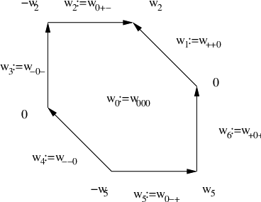
Here is a basis of eigenvectors in the case of three lines in the plane given by Theorem 3.6. The λℝ2\lambda_{{\mathbb{R}}^{2}}-eigenvector is provided by qq of (2.7): if we specialize the weights to a probability distribution, recall 1=λℝ21=\lambda_{{\mathbb{R}}^{2}}, and the eigenvector is the stationary distribution (2.5).
For an arrangement of one point in a line, the vector (2.7) equals

(3.3) w++w0+w−w0​w+​w−​(w++w−)⋅(w+,w−),\frac{w_{\mathchar 43}+w_{0}+w_{\mathchar 512}}{w_{0}w_{\mathchar 43}w_{\mathchar 512}(w_{\mathchar 43}+w_{\mathchar 512})}\cdot(w_{\mathchar 43},w_{\mathchar 512}),

ordering the chambers with +{\mathchar 43} first. Let 𝐗=(ℝ2,H1){\mathbf{X}}=({\mathbb{R}}^{2},H_{1}). Then ΦH1​(𝐗)\Phi_{H_{1}}({\mathbf{X}}) is a unit multiple of w0+−​ϕ​(𝐗⊗C0+−)+w0−+​ϕ​(𝐗⊗C0−+)w_{0{\mathchar 43}{\mathchar 512}}\phi({\mathbf{X}}\otimes C_{0{\mathchar 43}{\mathchar 512}})+w_{0{\mathchar 512}{\mathchar 43}}\phi({\mathbf{X}}\otimes C_{0{\mathchar 512}{\mathchar 43}}), as in (3.3). Using the calculation in Example 2.18 gives the vector shown in Figure 4.

We order the basis of VV counterclockwise, starting with the chamber +++{\mathchar 43}{\mathchar 43}{\mathchar 43}. For clarity, the weights of the codimension-00 and -11 faces are relabelled w0,…,w6w_{0},\ldots,w_{6} as shown in Figure 4. Then the eigenvectors given by Theorem 3.6 are

𝐗Ψ⁡(𝐗)​ proportional toλ(ℝ2)p, above∑i=06wi(ℝ2,H1)(0,w2,−w2,0,−w5,w5)w0+w2+w5(ℝ2,H2)(w6,0,w3,−w3,0,−w6)w0+w3+w6(ℝ2,H3)(−w1,w1,0,w4,−w4,0)w0+w1+w4(ℝ2,H1,0)(0,−1,1,0,−1,1)w0(ℝ2,H2,0)(1,0,−1,1,0,−1)w0\begin{array}[]{c|c|c}{\mathbf{X}}&\Psi({\mathbf{X}})\text{~proportional to}&\lambda\\ \hline\cr({\mathbb{R}}^{2})&p,\text{~above}&\sum_{i=0}^{6}w_{i}\\ \hline\cr({\mathbb{R}}^{2},H_{1})&(0,w_{2},-w_{2},0,-w_{5},w_{5})&w_{0}+w_{2}+w_{5}\\ ({\mathbb{R}}^{2},H_{2})&(w_{6},0,w_{3},-w_{3},0,-w_{6})&w_{0}+w_{3}+w_{6}\\ ({\mathbb{R}}^{2},H_{3})&(-w_{1},w_{1},0,w_{4},-w_{4},0)&w_{0}+w_{1}+w_{4}\\ \hline\cr({\mathbb{R}}^{2},H_{1},0)&(0,-1,1,0,-1,1)&w_{0}\\ ({\mathbb{R}}^{2},H_{2},0)&(1,0,-1,1,0,-1)&w_{0}\end{array}
Refer to caption
Figure 4. ΨH1​(ℝ2,H1)\Psi_{H_{1}}({\mathbb{R}}^{2},H_{1}) in Example 3.8
Remark 3.9.

The results of [10] on which Theorem 3.6 is based can likely be generalized to arbitrary oriented matroids without change, in which case the results here would generalize in the same way: see the discussion in [3].

In [2], Brown shows that many of the BHR random walk’s properties (such as diagonalizability) can also be generalized by replacing the face algebra with any semigroup with the left-regular band property. The same paper describes idempotents for irreducible modules, which implicitly give eigenvectors for the generalized random walk. However, that description is somewhat more complicated than the one here. Recent work of Saliola [8] gives a quite different description of the eigenvectors of the BHR random walk, using methods that hold for any left-regular band. His construction is complementary to the one given here. The cost of working with the general setting of [2] is apparently no longer to have an eigenbasis with such convenient labelling as non-broken circuits. It would be interesting to know, then, if the main results of [10] would admit left-regular band generalizations.

Acknowledgment.

The author would like to thank Phil Hanlon for helpful discussions at the start of this project, and the Institut de Géométrie, Algèbre et Topologie at the EPFL for its hospitality during its completion.

References

  • [1] Pat Bidigare, Phil Hanlon, Dan Rockmore, A combinatorial description of the spectrum for the Tsetlin library and its generalization to hyperplane arrangements, Duke Math. J. 99 (1999), 135–174.
  • [2] Kenneth S. Brown, Semigroups, rings, and Markov chains, J. Theoret. Probab. 13 (2000), 871–938.
  • [3] Kenneth S. Brown, Persi Diaconis, Random walks and hyperplane arrangements, Ann. Probab. 26 (1998), 1813–1854.
  • [4] Graham Denham, The Orlik-Solomon complex and Milnor fibre homology, Topology Appl. 118 (2002), 45–63, Arrangements in Boston: a Conference on Hyperplane Arrangements (1999).
  • [5] P. McMullen, On zonotopes, Trans. Amer. Math. Soc. 159 (1971), 91–109.
  • [6] P. Orlik, H. Terao, Arrangements of hyperplanes, Grundlehren der Mathematischen Wissenschaften, no. 300, Springer-Verlag, 1992.
  • [7] Nicholas Proudfoot, The equivariant Orlik-Solomon algebra, J. Algebra 305 (2006), 1186–1196.
  • [8] Franco Saliola, Eigenvectors for a random walk on a left-regular band, this volume, 2011.
  • [9] Vadim V. Schechtman, Alexander N. Varchenko, Arrangements of hyperplanes and Lie algebra homology, Invent. Math. 106 (1991), 139–194.
  • [10] A. N. Varchenko, I. M. Gel′fand, Heaviside functions of a configuration of hyperplanes, Functional Anal. Appl. 21 (1987), 255–270.
  • [11] Alexandre Varchenko, Bilinear form of real configuration of hyperplanes, Adv. Math. 97 (1993), 110–144.
  • [12] Günter M. Ziegler, Lectures on polytopes, Graduate Texts in Mathematics, vol. 152, Springer-Verlag, New York, 1995.