A summary is reported on our previous publications about four-dimensional ${\cal N}=1$ supersymmetric $Spin(10)$ gauge theory with chiral superfields in the spinor and vector representations in the non-Abelian Coulomb phase. Carrying out the method of $a$ -maximization, we studied decoupling operators in the infrared and the renormalization flow of the theory.
We also give a brief review on the non-Abelian Coulomb phase of the theory after recalling the unitarity bound and the $a$ -maximization procedure in four-dimensional conformal field theory.

This is a review article invited to International Journal of Modern Physics A.

October, 2010

Chapter 1 Introduction

Four-dimensional ${\cal N}=1$ $Spin$ (10) gauge theory with one chiral superfield in the spinor representation and $N_{Q}$ chiral superfields in the vector representation has rich and intriguing dynamics. In particular, for no vector representations, supersymmetry is dynamically broken [1, 2]. For $7\leq{N}_{Q}\leq 21$ vectors, the theory is in the non-Abelian Coulomb phase, and has a dual description at the non-trivial fixed point [3, 4]. It also leads at some points in the moduli space to the duality [5] between chiral and vector-like gauge theories, as well as the one discussed in [6]. The analysis has been extended for more spinors in [7].

When an ${\cal N}=1$ supersymmetric theory is in the non-Abelian Coulomb phase, it must be left invariant under conformal transformations at a non-trivial infrared fixed point, and ${\cal N}=1$ superconformal symmetry facilitates to obtain some exact results about the theory. In particular, the scaling dimension $D({\cal O})$ of a gauge invariant chiral primary operator ${\cal O}$ can be determined by its $U(1)_{R}$ charge $R({\cal O})$ as

{D({\cal O})={3\over 2}R({\cal O}).}

The unitarity of representations of conformal symmetry [8] requires the scaling dimension $D({\cal O})$ of a scalar field ${\cal O}$ to satisfy

{D({\cal O})\geq 1.}

However, one sometimes encounters a gauge invariant chiral primary spinless operator ${\cal O}$ which appears to violate the inequality $R({\cal O})\geq 2/3$ . It has been discussed that such an operator decouples as a free field from the remaining interacting system, and an accidental $U(1)$ symmetry is enhanced in the infrared to fix the $U(1)_{R}$ charge of the operator ${\cal O}$ to $2/3$ [9, 10, 11].

One can see that one of the examples is $Spin$ (7) gauge theory with $N_{f}=7$ spinors $Q^{i}$ ( $i=1,\cdots,N_{f}$ ) and with no superpotential, where electric-magnetic duality was found for $7\leq{N_{f}}\leq 14$ in [5]. Its dual or magnetic theory is an $SU(N_{f}-4)$ gauge theory with $N_{f}$ antifundamentals $\bar{q}_{i}$ and a single symmetric tensor $s$ , along with gauge singlets $M^{ij}$ , which can be identified with $Q^{i}Q^{j}$ in the electric theory. The superpotential $W_{\rm mag}$ of the magnetic theory is given by

{W_{\rm mag}={\tilde{h}\over\tilde{\mu}^{2}}M^{ij}\bar{q}_{i}\,{s}\,\bar{q}_{j}+{1\over\tilde{\mu}^{N_{f}-7}}\det{s},}

where $\tilde{\mu}$ is a dimensionful parameter to give the correct mass dimension to $M^{ij}$ , and the dimensionless parameter $\tilde{h}$ shows up because we assume that the field $M^{ij}$ has the canonical kinetic term.

Since the $U(1)_{R}$ charge of the spinors $Q^{i}$ is given by $1-(5/N_{f})$ , the gauge invariant operator $M^{ij}$ appears to violate the unitarity bound for $N_{f}=7$ and therefore propagates as a free field at the infrared fixed point.

In the magnetic theory, it suggests that the coupling $\tilde{h}$ in the superpotential $W_{\rm mag}$ goes to zero in the infrared. Therefore, at the infrared fixed point, the superpotential of the magnetic theory becomes

\displaystyle W_{\rm IR}={1\over\tilde{\mu}^{N_{f}-7}}\det{s}.

Contrary to the electric theory, on the magnetic side, the gauge invariant operator $M^{ij}$ is an elementary field. Therefore, the vanishing of the coupling $\tilde{h}$ implies that $M^{ij}$ may be a free field.

On the contrary, suppose that we start with the superpotential $W_{\rm IR}$ at the infrared fixed point. The fields $\bar{q}_{i}$ and $s$ are still interacting, and the $U(1)_{R}$ charge $2-2(1-(5/N_{f}))=10/N_{f}$ of $\bar{q}_{i}\,s\,\bar{q}_{j}$ is greater than $2-(2/3)$ for $N_{f}=7$ . Let us introduce an elementary field $M_{ij}$ , which carries $U(1)_{R}$ charge $2/3$ , as $M_{ij}$ is a free field. Therefore, the interaction $M^{ij}\bar{q}_{i}\,s\,\bar{q}_{j}$ is an irrelevant operator in the superpotential at the infrared fixed point, and it is consistent with the implication of the unitarity bound for the operator $M^{ij}$ .

One thus sees that the magnetic description yields a simple explanation of the prescription [11] for a composite operator hitting the unitarity bound, which has been explained by using the auxiliary field method [12]. The prescription [11] and the explanation [12] will be described in section 2.3.

Furthermore, when $\tilde{h}$ vanishes, one no longer has the F-term condition

{{\tilde{h}\over\tilde{\mu}^{2}}\,\bar{q}_{i}\,s\,\bar{q}_{j}={\partial W_{\rm mag}\over\partial M^{ij}}=0,}

and thus the gauge invariant operators $N_{ij}=\bar{q}_{i}\,s\,\bar{q}_{j}$ becomes a non-trivial chiral primary operator at the infrared fixed point. One can easily see that the resulting magnetic theory at the fixed point has a different electric dual from the original electric theory with no superpotential.

In fact, its electric dual is the same as the original electric theory except that it has the non-zero superpotential

{W_{{\rm ele}}={1\over\mu}N_{ij}Q^{i}Q^{j},}

along with free singlets $M^{ij}$ . Thus, one can conclude that these two electric theories are identical at the infrared fixed point. It also means that the original dual pair of the $Spin(7)$ gauge theory with no superpotential and the magnetic theory with the superpotential $W_{\rm mag}$ flows into another dual pair of the $Spin(7)$ theory with the superpotential $W_{{\rm ele}}$ and the magnetic dual with vanishing $\tilde{h}$ in the superpotential in the infrared.

We have thus seen that the $U(1)_{R}$ charge assignments were very important to understand the decoupling operator and the renormalization flow of the theory. However, when a superconformal field theory is also invariant under other global $U(1)$ symmetries besides the $U(1)_{R}$ symmetry, which linear combination of those $U(1)$ generators yields the superconformal $U(1)_{R}$ symmetry is dynamically determined. In [13], Intriligator and Wecht has proposed the method of $a$ -maximization to pick up the superconformal $U(1)_{R}$ generator among all the linear combinations of the $U(1)$ generators.

In this review article, we will give a summary on our previous publications [14, 15] about the non-Abelian Coulomb phase of four-dimensional ${\cal N}=1$ supersymmetric $Spin(10)$ gauge theories with one and two chiral superfields in the spinor representation and $N_{Q}$ chiral fields in the vector representation. They are invariant under two global $U(1)$ symmetries, and one needs to apply $a$ -maximization to determine the superconformal $U(1)_{R}$ symmetry.

In chapter 2, we give a brief review on ${\cal N}=1$ superconformal algebra and its lowest weight representations. We will discuss the unitarity of representations of the conformal algebra, following [16, 17] to give the unitarity bound, although a complete derivation [8] of it will not be given in this article. The relation of chiral primary operators to a chiral ring will be explained. After giving the definition of the conformal anomalies or the central charges $c$ and $a$ in four dimensions and recalling their relation [18, 19] to the ’t Hooft anomalies, we will explain the method of $a$ -maximization [13] in some detail.

In chapter 3, we will review the non-Abelian Coulomb phase of the supersymmetric $Spin(10)$ theory with one spinor and $7\leq{N_{Q}}\leq 21$ vectors [3, 4] in section 3.1 and the one with two spinors and $6\leq{N_{Q}}\leq 19$ vectors [7] in section 3.2. Their dual descriptions [3, 4, 7] at the infrared fixed point will briefly be explained. In chapter 4, we will describe our results obtained by the application of $a$ -maximization to the theories.

In chapter 5, we will discuss consistency checks about our results and their implication for the renormalization flow of the theories, as discussed above for the $Spin(7)$ theory. In particular, one will note in the $Spin(10)$ theory that the decoupling meson operator is given by an elementary field on the magnetic side, which also yields a simple explanation for the prescription [11], as in the $Spin(7)$ theory. In addition, we will use the auxiliary field method on the electric side to attempt to describe the decoupling of the composite meson operator. The flow of the electric-magnetic dual pair into another pair will also be seen in the $Spin(10)$ theory.

Chapter 6 will be devoted to our summary and outlook.

Chapter 2 ${\cal N}=1$ Superconformal Field Theory

2.1 ${\cal N}=1$ Superconformal Algebra

In this section, we will briefly review basic facts about four-dimensional ${\cal N}=1$ superconformal algebra. They will frequently be used in the rest of this article.

Conformal transformations are defined, upon acting on the spacetime coordinates $x^{\mu}$ , as those preserving the metric $\eta_{\mu\nu}$ up to an overall nowhere-zero function $\Omega^{2}(x)$ . The metric $\eta_{\mu\nu}$ thus transforms under a conformal transformation as

\displaystyle ds^{2}=\eta_{\mu\nu}dx^{\mu}dx^{\nu}\,\,\to\,\,ds^{\prime}{}^{2}=\eta_{\mu\nu}dx^{\prime}{}^{\mu}dx^{\prime}{}^{\nu}=\Omega^{2}(x)\eta_{\mu\nu}dx^{\mu}dx^{\nu}.

(2.1)

They all are generated by the infinitesimal transformations

\displaystyle\begin{array}[]{lcl}\mathrm{Lorentz\,\,transformation}&:&x^{\prime}{}^{\mu}=x^{\mu}-\omega^{\mu\nu}x_{\nu},\cr\mathrm{Dilatation\,(Dilation)}&:&x^{\prime}{}^{\mu}=(1-\varepsilon)x^{\mu},\cr\mathrm{Translation}&:&x^{\prime}{}^{\mu}=x^{\mu}+a^{\mu},\cr\mathrm{Special\,\,conformal\,\,transformation}&:&x^{\prime}{}^{\mu}=x^{\mu}-2b^{\nu}x_{\nu}x^{\mu}+b^{\mu}x^{\nu}x_{\nu},\end{array}

and thus the generators of them can be read as

\displaystyle\begin{array}[]{lcl}\mathrm{Lorentz\,\,transformation}&:&M_{\mu\nu}=-i(x_{\mu}\partial_{\nu}-x_{\nu}\partial_{\mu}),\cr\mathrm{Dilatation\,(Dilation)}&:&D=ix^{\nu}\partial_{\nu},\cr\mathrm{Translation}&:&P_{\mu}=-i\partial_{\mu},\cr\mathrm{Special\,\,conformal\,\,transformation}&:&K_{\mu}=-i(x^{2}\partial_{\mu}-2x_{\mu}x^{\nu}\partial_{\nu}),\end{array}

as a representation on the spacetime coordinates $x^{\mu}$ . They satisfy the commutation relations

	$\displaystyle[M_{\mu\nu},\,M_{\rho\sigma}]=i\left(\eta_{\mu\rho}M_{\nu\sigma}-\eta_{\mu\sigma}M_{\nu\rho}-\eta_{\nu\rho}M_{\mu\sigma}+\eta_{\nu\sigma}M_{\mu\rho}\right),$
	$\displaystyle[M_{\mu\nu},\,P_{\rho}]=i(\eta_{\mu\rho}P_{\nu}-\eta_{\nu\rho}P_{\mu}),\qquad[M_{\mu\nu},\,K_{\rho}]=i(\eta_{\mu\rho}K_{\nu}-\eta_{\nu\rho}K_{\mu}),$		(2.12)
	$\displaystyle[D,\,P_{\mu}]=-iP_{\mu},\qquad[D,\,K_{\mu}]=iK_{\mu},\qquad[D,\,M_{\mu\nu}]=0,$
	$\displaystyle[P_{\mu},\,P_{\nu}]=[K_{\mu},\,K_{\nu}]=0,\qquad[P_{\mu},\,K_{\nu}]=-2i\left(\eta_{\mu\nu}D+M_{\mu\nu}\right).$

They are isomorphic to the Lie algebra of $SO(2,4)$ , whose generators $S_{AB}$ ( $A,B=-1,\cdots,4$ ) satisfy

\displaystyle\left[S_{AB},\,S_{CD}\right]=i\left(\eta_{AC}S_{BD}-\eta_{AD}S_{BC}-\eta_{BC}S_{AD}+\eta_{BD}S_{AC}\right),

(2.13)

where $\eta_{ab}=\mathrm{diag}(-1,-1,1,1,1,1)$ . With the identification

\displaystyle S_{\mu\nu}=M_{\mu\nu},\qquad S_{\mu\,-1}=\frac{1}{2}(P_{\mu}+K_{\mu}),\qquad S_{\mu\,4}=\frac{1}{2}(P_{\mu}-K_{\mu}),\qquad S_{-1\,4}=D,

(2.14)

the algebra (2.13) is rewritten as the commutation relations (2.12) of the conformal algebra.

Considering a unitary representation of the conformal algebra (2.12) reveals a bound on its conformal dimension $d$ - the eigenvalue of the dilatation operator $D$ . All unitary irreducible representations with non-negative energy has been classified by Mack [8]. It was shown that such a representation always has the lowest weight state, and that all the representations are sorted into five classes, which are labeled by the conformal dimension $d$ and the spins $(j_{1},j_{2})$ of the Lorentz group $SL(2,\mathbf{C})$ of their lowest weight states, as listed in Table 2.1.

(1)

d=j_{1}=j_{2}=0

(2)

j_{1}\neq 0,j_{2}\neq 0,d>j_{1}+j_{2}+2

(3)

j_{1}j_{2}=0,d>j_{1}+j_{2}+1

(4)

j_{1}\neq 0,j_{2}\neq 0,d=j_{1}+j_{2}+2

(5)

j_{1}j_{2}=0,d=j_{1}+j_{2}+1

Table 2.1: Unitary irreducible representations

One can see from Table 2.1 that apart from the trivial identity operator in $(1)$ , the conformal dimension $d$ of an operator should satisfy

\displaystyle d\geq 1\quad{\rm for~scalar},\qquad d\geq\frac{3}{2}\quad{\rm for~spinor},\qquad d\geq 3\quad{\rm for~vector},

(2.15)

depending on the spin $(j_{1},j_{2})$ of the operator. These bounds on conformal dimensions are imposed by the unitarity of representations and are referred to as the unitarity bound. The inequalities are saturated if and only if their fields are free for the scalar and the spinor case. For the vector case, the equality is satisfied by a gauge invariant conserved current. We will frequently use the unitarity bound for a scalar field in our analysis in the following chapters.

We therefore will sketch a derivation of the unitary bounds. For a complete proof and detailed discussions¹¹ 1 Further restrictions have been discussed very recently in [20, 21, 22] , see [8, 16, 17]. The maximal compact subalgebra of the $SO(2,4)$ is given by $SO(2)\times{SO}(4)$ , whose generators can be taken as $S_{-10}$ for the $SO(2)$ and $S_{ab}$ ( $a,b=1,\cdots,4$ ) for the $SO(4)$ . The remaining generators of the $SO(2,4)$ are $S_{-1a}$ and $S_{0a}$ , which are combined to define

\displaystyle E_{a}^{\pm}=\left(S_{a-1}\mp{i}{S}_{a0}\right),

(2.16)

transforming in the representation $(\pm 1,{\bf 4})$ , respectively under the $SO(2)\times{SO}(4)$ rotations. From the commutation relations (2.13), one can see that these generators $E_{a}^{\pm}$ satisfy

\displaystyle\left[E_{a}^{-},\,E_{b}^{+}\right]=2\left(\delta_{ab}\,S_{-10}-i\,S_{ab}\right).

(2.17)

One thus, may regard $E_{a}^{+}$ and $E_{a}^{-}$ as a raising operator and a lowering operator, respectively. Since we assume that the generators $S_{AB}$ are all hermitian, $E_{a}^{+}$ and $E_{a}^{-}$ are adjoint to each other; $\left(E_{a}^{\pm}\right)^{{\dagger}}=E_{a}^{\mp}$ .

The $SO(4)$ algebra is isomorphic to the Lie algebra of $SU(2)\times{}SU(2)$ , and the generators are given by two copies of $SU(2)$ generators $S^{(1)}_{i}$ , $S^{(2)}_{i}$ ( $i=1,2,3$ ) defined by

\displaystyle S_{i}^{(1)}={1\over 2}\left({1\over 2}\epsilon_{ikl4}S_{kl}-S_{i4}\right),\qquad S_{i}^{(2)}={1\over 2}\left({1\over 2}\epsilon_{ikl4}S_{kl}+S_{i4}\right).

(2.18)

A state of a unitary irreducible representation of the $SO(2)\times{SO}(4)$ algebra is specified with eigenvalue $d$ of $S_{-10}$ and two pairs of spin quantum numbers $(j_{1},m_{1})$ and $(j_{2},m_{2})$ , and is denoted as $\left|{d;j_{1},m_{1};j_{2},m_{2}}\right\rangle$ . In particular, for the lowest weight state $\left|{d;j_{1},-j_{1};j_{2},-j_{2}}\right\rangle$ of the unitary irreducible representation, we will adopt a convention of writing simply $\left|{d,j_{1},j_{2}}\right\rangle$ as shorthand.

A unitary irreducible representation of the $SO(2,4)$ algebra may be given by a set of unitary irreducible representations of the $SO(2)\times{SO}(4)$ subalgebra. The unitary irreducible representations of the $SO(2)\times{SO}(4)$ can be specified by the lowest weight state $\left|{d,j_{1},j_{2}}\right\rangle$ of each of them. A unitary irreducible representation of the $SO(2)\times{SO}(4)$ contained in a unitary irreducible representation of the $SO(2,4)$ algebra may be mapped by the ladder operators $E_{a}^{\pm}$ into another unitary irreducible representation of the $SO(2)\times{SO}(4)$ in the same representation of the $SO(2,4)$ algebra.

Among unitary irreducible representations of the $SO(2)\times{SO}(4)$ in a unitary irreducible representation of the $SO(2,4)$ algebra, let us pick up the unitary irreducible representation of the $SO(2)\times{SO}(4)$ specified by the lowest weight state $\left|{d,j_{1},j_{2}}\right\rangle$ with the lowest value of $d$ . Since the lowering operators $E_{a}^{-}$ carry charge $-1$ of the $SO(2)$ , the lowest weight state $\left|{d,j_{1},j_{2}}\right\rangle$ must be annihilated by the $E_{a}^{-}$ , because there are no lowest weight states with lower eigenvalues of $S_{-10}$ than $d$ in the unitary irreducible representation of the $SO(2,4)$ .

Then the first non-trivial state one would like to study about its unitarity would be $E_{a}^{+}\left|{d,j_{1},j_{2}}\right\rangle$ . The unitarity requires the matrix

	$\displaystyle M_{(m^{\prime}_{1},m^{\prime}_{2},a)\,(m_{1},m_{2},b)}$	$\displaystyle=$	$\displaystyle\left\langle{d;j_{1},m^{\prime}_{1};j_{2},m^{\prime}_{2}}\right\|{E}_{a}^{-}E_{b}^{+}\left\|{d;j_{1},m_{1};j_{2},m_{2}}\right\rangle$		(2.19)
		$\displaystyle=$	$\displaystyle\left\langle{d;j_{1},m^{\prime}_{1};j_{2},m^{\prime}_{2}}\right\|\left[E_{a}^{-},\,E_{b}^{+}\right]\left\|{d;j_{1},m_{1};j_{2},m_{2}}\right\rangle$		(2.19)

to be positive definite, if $E_{a}^{+}\left|{d,j_{1},j_{2}}\right\rangle$ is not vanishing. The commutator gives $2\left(\delta_{ab}\,S_{-10}-i\,S_{ab}\right)$ . Following Minwalla’s trick [16], let us recall that $-iS_{ab}$ may be rewritten as

-iS_{ab}=-{i\over 2}\left(\delta_{ac}\delta_{bd}-\delta_{ad}\delta_{bc}\right)S_{cd}={1\over 2}\left(S_{cd}\right)_{ab}S_{cd}

and that $\left(\left(S_{cd}\right)_{ab}\right)$ is a matrix in the representation ${\bf 4}$ of $S_{cd}$ . The representation ${\bf 4}$ of the $SO(4)$ algebra is the spins $(j_{1}={1/2},j_{2}={1/2})$ of the isomorphic $SU(2)\times{SU(2)}$ algebra, and the matrices $\left(\delta_{ab}\right)$ and $\left(\left(S_{cd}\right)_{ab}\right)$ can be regarded as the matrix elements of the identity operator and the generator $S_{cd}$ ;

	$\displaystyle\delta_{ab}\quad\to\quad\left\langle{\alpha^{\prime}_{1},\alpha^{\prime}_{2}}\right\|{1\hskip-3.0pt{\rm l}}\left\|{\alpha_{1},\alpha_{2}}\right\rangle,$
	$\displaystyle\left(S_{cd}\right)_{ab}\quad\to\quad\left\langle{\alpha^{\prime}_{1},\alpha^{\prime}_{2}}\right\|S_{cd}\left\|{\alpha_{1},\alpha_{2}}\right\rangle,$		(2.20)

where the state $\left|{\alpha_{1},\alpha_{2}}\right\rangle$ is a shorthand for $\left|{j_{1}={1/2},\alpha_{1};j_{2}={1/2},\alpha_{2}}\right\rangle$ , and the similar shorthand was also used for the bra states. The matrix $M_{(m^{\prime}_{1},m^{\prime}_{2},a)\,(m_{1},m_{2},b)}$ is then given by the operator $2{1\hskip-3.0pt{\rm l}}\otimes{D}+S_{cd}\otimes{S}_{cd}$ sandwiched by the bra $\left\langle{\alpha^{\prime}_{1},\alpha^{\prime}_{2}}\right|\otimes\left\langle{d;j_{1},m^{\prime}_{1};j_{2},m^{\prime}_{2}}\right|$ and the ket $\left|{\alpha_{1},\alpha_{2}}\right\rangle\otimes\left|{d;j_{1},m_{1};j_{2},m_{2}}\right\rangle$ . The tensor product $S_{cd}\otimes{S}_{cd}$ may be rewritten as

S_{cd}\otimes{S}_{cd}={1\over 2}\left[\left(S_{cd}\otimes{1\hskip-3.0pt{\rm l}}+{1\hskip-3.0pt{\rm l}}\otimes{S}_{cd}\right)^{2}-\left(S_{cd}\otimes{1\hskip-3.0pt{\rm l}}\right)^{2}-\left({1\hskip-3.0pt{\rm l}}\otimes{S}_{cd}\right)^{2}\right],

and one thus finds that the matrix $M_{(m^{\prime}_{1},m^{\prime}_{2},a)\,(m_{1},m_{2},b)}$ is given by

\left\langle{\alpha^{\prime}_{1},\alpha^{\prime}_{2},m^{\prime}_{1},m^{\prime}_{2}}\right|2\left[{1\hskip-3.0pt{\rm l}}\otimes{D}+{1\over 4}\left[\left(S_{cd}\otimes{1\hskip-3.0pt{\rm l}}+{1\hskip-3.0pt{\rm l}}\otimes{S}_{cd}\right)^{2}-\left(S_{cd}\otimes{1\hskip-3.0pt{\rm l}}\right)^{2}-\left({1\hskip-3.0pt{\rm l}}\otimes{S}_{cd}\right)^{2}\right]\right]\left|{\alpha_{1},\alpha_{2},m_{1},m_{2}}\right\rangle

with a shorthand $\left|{\alpha_{1},\alpha_{2},m_{1},m_{2}}\right\rangle$ for $\left|{\alpha_{1},\alpha_{2}}\right\rangle\otimes\left|{d;j_{1},m_{1};j_{2},m_{2}}\right\rangle$ and $\left\langle{\alpha^{\prime}_{1},\alpha^{\prime}_{2},m^{\prime}_{1},m^{\prime}_{2}}\right|$ for $\left\langle{\alpha^{\prime}_{1},\alpha^{\prime}_{2}}\right|\otimes\left\langle{d;j_{1},m^{\prime}_{1};j_{2},m^{\prime}_{2}}\right|$ . The ket $\left|{\alpha_{1},\alpha_{2}}\right\rangle\otimes\left|{d;j_{1},m_{1};j_{2},m_{2}}\right\rangle$ is in the representation $({1\over 2},{1\over 2})\otimes(j_{1},j_{2})$ , which is decomposed into irreducible representations as

(j_{1}+{1\over 2},j_{2}+{1\over 2})\oplus(j_{1}+{1\over 2},j_{2}-{1\over 2})\oplus(j_{1}-{1\over 2},j_{2}+{1\over 2})\oplus(j_{1}-{1\over 2},j_{2}-{1\over 2})

for $j_{1}\geq 1/2$ and $j_{2}\geq 1/2$ . Using elementary facts of the $SU(2)$ spin operators

{1\over 4}\left(S_{cd}\right)^{2}=\sum_{i=1}^{3}\left[\left(S^{(1)}_{i}\right)^{2}+\left(S^{(2)}_{i}\right)^{2}\right]

and

\sum_{i=1}^{3}\left(S_{i}\right)^{2}\left|j,m\right\rangle=j(j+1)\left|j,m\right\rangle,

one can see that, among the operators in the above expression of the matrix $M_{(m^{\prime}_{1},m^{\prime}_{2},a)\,(m_{1},m_{2},b)}$ , only $\left(S_{cd}\otimes{1\hskip-3.0pt{\rm l}}+{1\hskip-3.0pt{\rm l}}\otimes{S}_{cd}\right)^{2}$ depends on the above irreducible representations to give its eigenvalues. The contribution from the other operators yields

2\left[d-2\times{3\over 4}-j_{1}(j_{1}+1)-j_{2}(j_{2}+1)\right],

and the operator $\left(S_{cd}\otimes{1\hskip-3.0pt{\rm l}}+{1\hskip-3.0pt{\rm l}}\otimes{S}_{cd}\right)^{2}$ takes the minimal value in $(j_{1}-{1\over 2},j_{2}-{1\over 2})$ for $j_{1}\geq 1/2$ and $j_{2}\geq 1/2$ among the four irreducible representations to contribute

2\left[(j_{1}-{1\over 2})(j_{1}+{1\over 2})+(j_{2}-{1\over 2})(j_{2}+{1\over 2})\right]

to the matrix $M_{(m^{\prime}_{1},m^{\prime}_{2},a)\,(m_{1},m_{2},b)}$ . One obtains the total contribution

2\left(d-j_{1}-j_{2}-2\right)

to it. For $j=j_{1}\geq 1/2$ and $j_{2}=0$ , or for $j=j_{2}\geq 1/2$ and $j_{1}=0$ , the minimal value of $\left(S_{cd}\otimes{1\hskip-3.0pt{\rm l}}+{1\hskip-3.0pt{\rm l}}\otimes{S}_{cd}\right)^{2}$ similarly contributes

2\left[(j-{1\over 2})(j+{1\over 2})+{3\over 4}\right]

to give the total contribution

2\left[d+(j-{1\over 2})(j+{1\over 2})-j(j+1)-{3\over 4}\right]=2\left(d-j-1\right),

while it is obvious that the total contribution is $2d$ for a scalar $j_{1}=j_{2}=0$ .

The requirement that the eigenvalues of the matrix $M_{(m^{\prime}_{1},m^{\prime}_{2},a)\,(m_{1},m_{2},b)}$ be non-negative gives the inequalities

	$\displaystyle d\geq j_{1}+j_{2}+2\qquad(j_{1}\geq{1\over 2},j_{2}\geq{1\over 2}),$
	$\displaystyle d\geq j+1\qquad\qquad~(j=j_{1}\geq{1\over 2},j_{2}=0~{\rm or}~j_{1}=0,j=j_{2}\geq{1\over 2}),$
	$\displaystyle d\geq 0\qquad\qquad\qquad(j_{1}=0,j_{2}=0).$		(2.21)

The equality is satisfied by the trivial state

\displaystyle E_{a}^{+}\left|{d,j_{1},j_{2}}\right\rangle=0.

(2.22)

Converting the vector index of $E_{a}^{+}$ to a pair of spinor indices $(\alpha_{1},\alpha_{2})$ of the $SU(2)\times{SU(2)}$ , and also $\left|{d;j_{1},m_{1};j_{2},m_{2}}\right\rangle$ to $\left|{d;\beta_{1},\cdots,\beta_{2j_{1}};\gamma_{1},\cdots,\gamma_{2j_{2}}}\right\rangle$ , one can make the condition (2.22) more precise. In fact, for $j_{1}\geq{1\over 2},j_{2}\geq{1\over 2}$ , since the irreducible representation $(j_{1}-{1\over 2},j_{2}-{1\over 2})$ gives the minimal eigenvalue, the condition (2.22) means the contraction of both the indices $\alpha_{1}$ and $\alpha_{2}$ with the ones of the state to form the $(j_{1}-{1\over 2},j_{2}-{1\over 2})$ appropriately. For the remaining cases but the $j_{1}=j_{2}=0$ , the contraction is done for either of the indices. There is no contraction for $j_{1}=j_{2}=0$ , and (2.22) means that the representation with $d=j_{1}=j_{2}=0$ must be one-dimensional.

The inequalities (2.21) are the necessary condition for the lowest weight representation to be unitary, but it is also the sufficient condition except for the scalar case $j_{1}=j_{2}=0$ , which has been proved by Mack [8]. The inequalities (2.21) for those cases are referred to as the unitarity bounds, as mentioned before.

In order to obtain the unitarity bound for $j_{1}=j_{2}=0$ , among the next non-trivial states, let us take the state $\sum_{a}E_{a}^{+}E_{a}^{+}\left|{d,j_{1}=0,j_{2}=0}\right\rangle$ to calculate the norm

	$\displaystyle\sum_{a,b}\left\langle{d,0,0}\right\|{E}_{a}^{-}{E}_{a}^{-}E_{b}^{+}E_{b}^{+}\left\|{d,0,0}\right\rangle=32\,\left\langle{d,0,0}\right\|\Big[\left(S_{-10}\right)^{2}-S_{-10}\Big]\left\|{d,0,0}\right\rangle$
	$\displaystyle\quad=32\left(d^{2}-d\right)\,\left\langle{d,0,0}\right.\left\|{d,0,0}\right\rangle.$		(2.23)

The unitarity then requires that

\displaystyle d(d-1)\geq 0.

(2.24)

Therefore, if a state $\left|{d,j_{1}=0,j_{2}=0}\right\rangle$ is not trivial, the unitarity requires that

\displaystyle d\geq 1.

(2.25)

It is the unitarity bound [8] for a scalar field. In particular, the equality $d=1$ is satisfied if and only if

\displaystyle\sum_{a=1}^{4}E^{+}_{a}E^{+}_{a}|d,0,0\rangle=0.

(2.26)

So far we have been discussing eigenvalues of the operator $S_{-10}$ , as well as spins $(j_{1},j_{2})$ of the $SO(4)$ subalgebra, but we would like to relate them to eigenvalue of the dilatation generator $D=S_{-14}$ of the $SO(1,1)$ subgroup and spins of the algebra of the Lorentz group $SO(1,3)$ . It can be done by a similarity transformation [17] exchanging the coordinates $x^{0}$ and $x^{4}$ . In fact, the similarity transformation

	$\displaystyle iS_{0J}=e^{{\pi\over 2}S_{40}}S_{4J}e^{-{\pi\over 2}S_{40}},\qquad iS_{4J}=e^{{\pi\over 2}S_{40}}S_{0J}e^{-{\pi\over 2}S_{40}},$
	$\displaystyle S_{IJ}=e^{{\pi\over 2}S_{40}}S_{IJ}e^{-{\pi\over 2}S_{40}},\qquad S_{40}=e^{{\pi\over 2}S_{40}}S_{40}e^{-{\pi\over 2}S_{40}},\quad(I,J=-1,1,2,3)$		(2.27)

relates the operators $D$ , $P_{\mu}$ and $K_{\mu}$ to $S_{-10}$ , $E^{\pm}_{a}$ as

	$\displaystyle D=-ie^{{\pi\over 2}S_{40}}S_{-10}e^{-{\pi\over 2}S_{40}},$
	$\displaystyle iP_{0}=e^{{\pi\over 2}S_{40}}E^{+}_{4}e^{-{\pi\over 2}S_{40}},\qquad P_{i}=e^{{\pi\over 2}S_{40}}E^{+}_{i}e^{-{\pi\over 2}S_{40}},$
	$\displaystyle iK_{0}=e^{{\pi\over 2}S_{40}}E^{-}_{4}e^{-{\pi\over 2}S_{40}},\qquad K_{i}=e^{{\pi\over 2}S_{40}}E^{-}_{i}e^{-{\pi\over 2}S_{40}}.$		(2.28)

Incidentally, the spin operators $J^{(1)}_{i}$ , $J^{(2)}_{i}$ ( $i=1,2,3$ ) of the Lorentz group $SO(1,3)$ are given by

\displaystyle J_{i}^{(1)}={1\over 2}\left({1\over 2}\epsilon_{ikl}M_{kl}-iM_{i0}\right),\qquad J_{i}^{(2)}={1\over 2}\left({1\over 2}\epsilon_{ikl}M_{kl}+iM_{i0}\right),

and they are related to the $SO(4)$ spin operators $S^{(1)}_{i}$ , $S^{(2)}_{i}$ ( $i=1,2,3$ ) as

\displaystyle J_{i}^{(1)}=e^{{\pi\over 2}S_{40}}S_{i}^{(1)}e^{-{\pi\over 2}S_{40}},\qquad J_{i}^{(2)}=e^{{\pi\over 2}S_{40}}S_{i}^{(2)}e^{-{\pi\over 2}S_{40}}.

(2.29)

One then finds that an eigenstate $\left|{d;j_{1},m_{1};j_{2},m_{2}}\right\rangle$ of the original operators can be mapped to $\left|{d;j_{1},m_{1};j_{2},m_{2}}\right)=\exp((\pi/2)S_{40})\left|{d;j_{1},m_{1};j_{2},m_{2}}\right\rangle$ , which is an eigenstate ²² 2 In order for the generators $D$ , $P_{\mu}$ , $K_{\mu}$ , $M_{\mu\nu}$ to be hermitian, one needs to take the dual basis to be $\left({d;j_{1},m_{1};j_{2},m_{2}}\right|=\left\langle{d;j_{1},m_{1};j_{2},m_{2}}\right|\exp((\pi/2)S_{40})$ , as explained in [17]. of $D$ , $J^{L}_{3}$ and $J^{R}_{3}$ . In particular, one can see that the state $\left|{d;j_{1},m_{1};j_{2},m_{2}}{d,j_{1},j_{2}}\right)$ has Lorentz spins $(j_{1},m_{1};j_{2},m_{2})$ , and

\displaystyle D\left|{d;j_{1},m_{1};j_{2},m_{2}}\right)=-ie^{{\pi\over 2}S_{40}}S_{-10}\left|{d;j_{1},m_{1};j_{2},m_{2}}\right\rangle=-id\left|{d;j_{1},m_{1};j_{2},m_{2}}\right).

(2.30)

It means that under a dilatation $x^{\mu}\to{e}^{-a}x^{\mu}={e}^{iaD}x^{\mu}$ , the state $\left|{d;j_{1},m_{1};j_{2},m_{2}}\right)$ transforms as

\displaystyle\left|{d;j_{1},m_{1};j_{2},m_{2}}\right)\quad\to\quad e^{da}\left|{d;j_{1},m_{1};j_{2},m_{2}}\right),

(2.31)

which is consistent with the fact that it carries conformal dimension $d$ in the usual sense ³³ 3 Previously, we have referred to eigenvalue of the operator $D$ not $iD$ as conformal dimension less rigorously. But, this is the definition of conformal dimension, which we will use henceforth. .

Therefore, the conformal dimension $d$ of a scalar state $\left|{d,j_{1}=0,j_{2}=0}\right)$ must satisfy the unitarity bound (2.25). Since the state $\sum_{a=1}^{4}E^{+}_{a}E^{+}_{a}|d,0,0\rangle$ is transformed by the similarity transformation (2.27) to be $(-P_{0}P_{0}+\sum_{i=1}^{3}P_{i}P_{i})\left|d,0,0\right)$ , the condition (2.26) for $d=1$ yields

\displaystyle\eta^{\mu\nu}P_{\mu}P_{\nu}|d,0,0\rangle=0.

(2.32)

If one may regard the state $\left|d,0,0\right)$ as $\phi(0)\left|0,0,0\right)$ with a scalar field $\phi(x)$ , it suggests that

\displaystyle\partial^{\mu}\partial_{\mu}\phi(x)=0,

(2.33)

which is the free Klein-Gordon equation of a massless scalar field. The equality of the unitarity bound (2.25) is thus satisfied if and only if the field is free ⁴⁴ 4 For $(j_{1}=1/2,j_{2}=0)$ or $(j_{1}=0,j_{2}=1/2)$ , the condition (2.22) yields a free Dirac equation, while for $(j_{1}=1,j_{2}=0)$ or $(j_{1}=0,j_{2}=1)$ , it gives a free Maxwell equation. Finally, for $(j_{1}=1/2,j_{2}=1/2)$ , one finds the conservation law of a gauge invariant current. .

Let us proceed to the superconformal algebra. Besides the generators of the conformal algebra, there are the supersymmetry generator $Q_{\alpha}$ , the superconformal generator $S_{\dot{\alpha}}$ , and the superconformal $U(1)_{R}$ generator $R$ , which satisfy the commutation relations

	$\displaystyle\{Q_{\alpha},Q^{\dagger}_{\dot{\beta}}\}=2\sigma^{\mu}{}_{\alpha\dot{\beta}}P_{\mu},\qquad\{S_{\alpha},S_{\dot{\beta}}^{\dagger}\}=2\sigma^{\mu}{}_{\alpha\dot{\beta}}K_{\mu},$
	$\displaystyle[Q_{\alpha},K^{\mu}]=\sigma^{\mu}{}_{\alpha\dot{\beta}}S^{\dagger}{}^{\dot{\beta}},\qquad[S_{\alpha},P^{\mu}]=\sigma^{\mu}{}_{\alpha\dot{\beta}}Q^{\dagger}{}^{\dot{\beta}},$
	$\displaystyle[D,Q_{\alpha}]=-\frac{i}{2}Q_{\alpha},\quad[D,S_{\alpha}]=+\frac{i}{2}S_{\alpha},\quad[R,Q_{\alpha}]=-Q_{\alpha},\quad[R,S_{\alpha}]=+S_{\alpha},$
	$\displaystyle[Q_{\alpha},M^{\mu\nu}]=i\sigma^{\mu\nu}{}_{\alpha}{}^{\beta}Q_{\beta},\qquad[S_{\alpha},M^{\mu\nu}]=i\sigma^{\mu\nu}{}_{\alpha}{}^{\beta}S_{\beta},$
	$\displaystyle\{S_{\alpha},Q^{\beta}\}=-\delta_{\alpha}{}^{\beta}(2iD+3R)-2i\sigma^{\mu\nu}{}_{\alpha}{}^{\beta}M_{\mu\nu}.$		(2.34)

The superconformal algebra is isomorphic to the Lie superalgebra of $SU(2,2|1)$ . In addition to conformal dimension $d$ and spins $j_{1,2}$ , the superconformal $U(1)_{R}$ charge $r$ - the eigenvalue of $R$ - is used to specify a unitary irreducible representation with its lowest weight $(d,j_{1},j_{2},r)$ .

Since the superconformal algebra never closes without the superconformal $U(1)_{R}$ generator $R$ , any superconformal field theory must be invariant under the superconformal $U(1)_{R}$ transformation. Note that the superconformal $U(1)_{R}$ generator $R$ is unambiguously determined as in the right hand side of the commutation relation $\{S_{\alpha},Q^{\beta}\}$ . Therefore, even in a case where a superconformal field theory has more than one global $U(1)$ symmetry, the superconformal $U(1)_{R}$ charge should be singled out uniquely.

When a gauge theory is conformal invariant, it resides at an infrared fixed point, where the beta function of the gauge coupling $g$ must vanish. The NSVZ exact beta function of the coupling constant $g$ of a gauge group $G$ is given in [23] by

\displaystyle\beta(g)=-\frac{g^{3}}{16\pi^{2}}\frac{3T(G)-\sum_{i}T(r_{i})(1-\gamma_{i})}{1-T(G)({g^{2}}/{8\pi^{2}})},

(2.35)

where $\gamma_{i}$ is the anomalous dimension of a matter field labeled by $i$ . $T(\rho_{i})$ denotes the index of its representation $\rho_{i}$ , and $T(G)$ is the index of the adjoint representation ⁵⁵ 5 In our convention, ${\rm tr}_{\rho}(T^{A}_{\rho}{}T^{B}_{\rho})=T(\rho)\delta^{AB}$ with the normalization $T(G)=N$ for $G=SU(N)$ .. Its vanishing at the IR fixed point implies that the anomalous dimensions should satisfy

\displaystyle 3T(G)-\sum_{i}T(r_{i})(1-\gamma_{i})=0.

(2.36)

The anomalous dimension $\gamma_{i}$ at the infrared fixed point is related to the conformal dimension as $D_{i}=1+\gamma_{i}/2$ , and further can be given in terms of the $U(1)_{R}$ charge by $\gamma_{i}=3R_{i}-2$ , jumping ahead to (2.42). Thus, the equation (2.36) can be rewritten as

\displaystyle T(G)+\sum_{i}T(r_{i})(R_{i}-1)=0.

(2.37)

This is exactly the same as the anomaly free condition of the superconformal $U(1)_{R}$ symmetry. It guarantees that the superconformal $U(1)_{R}$ symmetry at the infrared fixed point does not suffer from anomalies caused by the gauge interaction.

In a superconformal field theory, several fields with different Lorentz spins are transformed with each other under superconformal transformations and form a superconformal multiplet. A local operator ${\cal O}(x)$ with the lowest conformal dimension in a superconformal multiplet is called a primary operator. It is known⁶⁶ 6 For a review on superconformal transformations, see e.g., [24]. that the other operators in the same irreducible superconformal multiplet can be obtained by successively acting the supersymmetry generators $Q_{\alpha}$ and $Q^{\dagger}_{\dot{\alpha}}$ on the primary operator.

Taking account of the commutation relations $[D,Q_{\alpha}]=-\frac{i}{2}Q_{\alpha}$ and $[D,S_{\alpha}]=+\frac{i}{2}S_{\alpha}$ in (2.34), one may regard the supersymmetry generators $Q_{\alpha},Q^{\dagger}_{\dot{\alpha}}$ as raising operators to raise conformal dimension, and the superconformal generators $S_{\alpha},S^{\dagger}_{\dot{\alpha}}$ as lowering operators. In fact, one can confirm this for an operator ${\cal O}$ of conformal dimension $d$ by the Jacobi identity

	$\displaystyle[D,[Q_{\alpha},{\cal O}\}\}$	$\displaystyle=$	$\displaystyle[[D,Q_{\alpha}],{\cal O}\}+[Q_{\alpha},[D,{\cal O}\}\}$		(2.38)
		$\displaystyle=$	$\displaystyle-\frac{i}{2}[Q_{\alpha},{\cal O}\}-id[Q_{\alpha},{\cal O}\}=-i\left(d+\frac{1}{2}\right)[Q_{\alpha},{\cal O}\}.$		(2.39)

Similarly, the commutation relations $[D,Q^{{\dagger}}_{\dot{\alpha}}]=-\frac{i}{2}Q^{{\dagger}}_{{\alpha}}$ and $[D,S^{{\dagger}}_{\dot{\alpha}}]=+\frac{i}{2}S^{{\dagger}}_{\dot{\alpha}}$ suggest that $Q^{{\dagger}}_{\dot{\alpha}}$ and $S^{\dagger}_{\dot{\alpha}}$ are raising and lowering operators, respectively.

As a primary operator has the lowest conformal dimension, it must satisfy the primary condition

\displaystyle[S_{\alpha},\,{\cal O}(0)\}=[S_{\dot{\alpha}}^{\dagger},\,{\cal O}(0)\}=0.

(2.40)

When the primary operator also satisfies the chiral condition

\displaystyle[Q^{\dagger}_{\dot{\alpha}},{\cal O}(0)\}=0,

(2.41)

it is referred to as a chiral primary operator.

A detailed study of unitary irreducible representations of the superconformal algebra [25, 26] shows that the inequality

{D({\cal O})\geq\frac{3}{2}R({\cal O})}

must be satisfied for any local scalar operator ${\cal O}(x)$ , where $D({\cal O})$ and $R({\cal O})$ are the conformal dimension and the $U(1)_{R}$ charge of the operator ${\cal O}(x)$ , respectively. It is remarkable that the equality

\displaystyle D({\cal O})=\frac{3}{2}R({\cal O})

(2.42)

is satisfied if and only if ${\cal O}(x)$ is a chiral primary operator.

Therefore, in particular, if the chiral primary operator carries no spin $(j_{1},j_{2})=(0,0)$ , the unitarity bound (2.25) means that

\displaystyle R({\cal O})\geq{2\over 3}.

(2.43)

In fact, one can obtain the equality (2.42) for a chiral primary operator ${\cal O}$ by calculating $[\{S^{\dagger}{}^{\dot{\alpha}},Q_{\dot{\beta}}^{\dagger}\},{\cal O}]$ in two different ways. On one hand, by using the commutation relation of the generators, one finds that

	$\displaystyle[\{S^{\dagger}{}^{\dot{\alpha}},Q_{\dot{\beta}}^{\dagger}\},{\cal O}]$	$\displaystyle=$	$\displaystyle[-\delta^{\dot{\alpha}}{}_{\dot{\beta}}(2iD-3R)-2i\bar{\sigma}_{\mu\nu}{}^{\dot{\alpha}}{}_{\dot{\beta}}M^{\mu\nu},{\cal O}]$		(2.44)
		$\displaystyle=$	$\displaystyle-\delta^{\dot{\alpha}}{}_{\dot{\beta}}(2d-3r){\cal O}.$		(2.45)

On the other hand, by using the Jacobi identity

\displaystyle[\{S^{\dagger}{}^{\dot{\alpha}},Q_{\dot{\beta}}^{\dagger}\},{\cal O}]=\{[Q_{\dot{\beta}}^{\dagger},{\cal O}],S^{\dagger}{}^{\dot{\alpha}}\}+\{[S^{\dagger}{}^{\dot{\alpha}},{\cal O}],Q_{\dot{\beta}}^{\dagger}\},

(2.46)

one can see that it vanishes due to the chiral condition and the primary condition. Thus, if ${\cal O}(x)$ is a chiral primary operator, the equality (2.42) is satisfied.

The relation (2.42) implies a striking fact - the additivity of the conformal dimensions of chiral primary operators. Since the $U(1)_{R}$ charge of the product of operators $O_{1}$ and $O_{2}$ is the sum of the charge of each operator;

R(O_{1}O_{2})=R(O_{1})+R(O_{2}),

their conformal dimensions must also be additive;

D(O_{1}O_{2})=D(O_{1})+D(O_{2}).

It suggests that the product of two chiral primary operators does not cause a singularity.

Since a product of chiral primary operators at a spacetime point is well-defined without any singularities - just a multiplication of them, all chiral primary operators can form a ring. In a supersymmetric gauge theory with a non-trivial infrared fixed point, it is in fact convenient to consider the set of all the chiral operators, which are not necessarily primary, and to introduce a quotient of the set by an equivalence relation, which we will refer to as a chiral ring. An equivalence class of the chiral ring is mapped into a chiral primary operator, as will be seen just below.

A chiral operator ${\cal O}$ satisfies the chiral condition

\displaystyle[Q^{\dagger}_{\dot{\alpha}},{\cal O}\}=0.

(2.47)

Then, we introduce the equivalence relation

\displaystyle{\cal O}\simeq{\cal O}+[Q^{\dagger}_{\dot{\alpha}},X^{\dot{\alpha}}\},

(2.48)

where $X^{\dot{\alpha}}$ is an arbitrary gauge invariant operator which satisfies

\displaystyle\left[Q^{\dagger}_{\dot{\beta}},[Q^{\dagger}_{\dot{\alpha}},X^{\dot{\alpha}}\}\right\}=0.

(2.49)

The chiral ring is the set consisting of all the gauge invariant chiral operators with the identification (2.48).

The term $[Q^{\dagger}_{\dot{\alpha}},X^{\dot{\alpha}}\}$ in (2.48) is not primary, because its conformal dimension is greater than that of $X^{\dot{\alpha}}$ , as $Q^{\dagger}_{\dot{\alpha}}$ carries conformal dimension a half. Since $X^{\dot{\alpha}}$ and $[Q^{\dagger}_{\dot{\alpha}},X^{\dot{\alpha}}\}$ reside in the same superconformal multiplet, $[Q^{\dagger}_{\dot{\alpha}},X^{\dot{\alpha}}\}$ is not primary. Conversely, a chiral non-primary operator ${\cal O}$ of conformal dimension $d$ and the superconformal $U(1)_{R}$ charge $r$ can be rewritten in a form $[Q^{\dagger}_{\dot{\alpha}},X^{\dot{\alpha}}\}$ . In fact, from (2.45) and (2.46) together with the chiral condition (2.41), one can show ⁷⁷ 7 Here, we assumed that ${\cal O}$ is a Lorentz scalar for simplicity. that

\displaystyle{\cal O}=-\frac{1}{2(2d-3r)}\{Q_{\dot{\beta}}^{\dagger},[S^{\dagger}{}^{\dot{\alpha}},{\cal O}]\},

(2.50)

where we used the fact that $2d>3r$ for a non-primary operator. It thus concludes that an equivalence class of the chiral ring corresponds to a chiral primary operator ⁸⁸ 8 The correspondence can also be seen by explicitly constructing a representation of the superconformal algebra on field operators. For a review, see e.g., [24]..

The condition (2.48) can be rewritten in terms of a chiral superfield $\Phi$ as

\displaystyle\Phi\simeq\Phi+\bar{\cal D}^{2}Z,

(2.51)

with $\bar{\cal D}^{2}=\bar{\cal D}_{\dot{\alpha}}\bar{\cal D}^{\dot{\alpha}}/2$ , where the supercovariant derivative $\bar{\cal D}_{\dot{\alpha}}$ is defined by using superspace coordinates $(x,\theta,\bar{\theta})$ as

\bar{\cal D}_{\dot{\alpha}}=\frac{\partial}{\partial\bar{\theta}^{\dot{\alpha}}}+i\theta^{\alpha}\sigma^{\mu}{}_{\alpha\dot{\alpha}}\partial_{\mu}.

This indicates that the lowest component of $\bar{\cal D}^{2}$ term is chiral but vanishes in the chiral ring.

Since it is generically formidable to consider the chiral ring at a non-trivial infrared fixed point, one often considers the chiral ring at the ultraviolet cutoff, which is referred to as a classical chiral ring. In the classical chiral ring, one assumes that a relation among gauge invariant operators is determined by the classical equations of motion. One can see that the equations of motion

\displaystyle\bar{\cal D}^{2}(\Phi^{\dagger}e^{V})+\frac{\partial W(\Phi)}{\partial\Phi}=0,

(2.52)

of the chiral superfield $\Phi$ yields the $F$ -term condition

\displaystyle\frac{\partial W(\Phi)}{\partial\Phi}\simeq 0,

(2.53)

as a defining equation of the classical chiral ring ⁹⁹ 9 Among gauge invariant operators including gaugino superfield $W_{\alpha}\propto\bar{\cal D}^{2}[e^{-V}{\cal D}_{\alpha}e^{V}]$ , there are other relations [27, 28] determined by $\displaystyle W_{\alpha}^{A}(T^{A})^{a}{}_{b}\,\phi^{b}\propto\bar{\cal D}^{2}\left[e^{-V}{\cal D}_{\alpha}(e^{V}\phi)\right]^{a}\sim 0,$ (2.54) where the matter field $\phi^{a}$ in the representation $\rho$ is labeled by the gauge index $a$ , and $T^{A}$ is the generator of the gauge group in the representation $\rho$ .. However, the classical defining equation (2.53) may be modified quantum mechanically. This deformed chiral ring is called a quantum chiral ring, which corresponds to the set of the chiral primary operators, as discussed previously.

2.2 Central Charges in Four-Dimensional Conformal Field Theories

In two-dimensional conformal field theories (CFTs), the central charge $c$ of the Virasoro algebra plays an important role. In a curved background, it is related to the trace anomaly as

\displaystyle\langle T^{\mu}{}_{\mu}\rangle=-\frac{c}{12}R,

(2.55)

where $R$ is the scalar curvature. In a four-dimensional conformal field theory, one also uses the trace anomaly to define the analogs of the two-dimensional central charge $c$ .

In four dimensions, the Weyl tensor $C_{\mu\nu\rho\sigma}$ is given in terms of the Riemann tensor $R_{\mu\nu\rho\sigma}$ as

\displaystyle C_{\mu\nu\rho\sigma}=R_{\mu\nu\rho\sigma}-\frac{1}{2}\left(g_{\mu\sigma}R_{\nu\rho}-g_{\mu\rho}R_{\nu\sigma}-g_{\nu\sigma}R_{\mu\rho}+g_{\nu\rho}R_{\mu\sigma}\right)+\frac{1}{3}(g_{\mu\sigma}g_{\nu\rho}-g_{\mu\rho}g_{\nu\sigma})R.

(2.56)

Using the dual $\tilde{R}^{\mu\nu\rho\sigma}=\varepsilon^{\mu\nu\alpha\beta}\varepsilon^{\rho\sigma\gamma\delta}R_{\alpha\beta\gamma\delta}/4$ of the Riemann tensor $R_{\mu\nu\rho\sigma}$ , the Euler density is defined by $(1/16\pi^{2})R_{\mu\nu\rho\sigma}\tilde{R}^{\mu\nu\rho\sigma}$ . The trace anomaly in a four-dimensional curved background is then calculated to be

\displaystyle\langle T^{\mu}{}_{\mu}\rangle=\frac{c}{16\pi^{2}}C_{\mu\nu\rho\sigma}C^{\mu\nu\rho\sigma}-\frac{a}{16\pi^{2}}R_{\mu\nu\rho\sigma}\tilde{R}^{\mu\nu\rho\sigma}.

(2.57)

The coefficients $a$ and $c$ are supposed to play a similar role to the two-dimensional $c$ , and are thus called the central charges of the four-dimensional CFT.

In a four-dimensional superconformal field theory, since one has the energy-momentum tensor $T_{\mu\nu}$ and the $U(1)_{R}$ current $J_{R}^{\mu}$ , the ’t Hooft anomaly coefficients Tr $R^{3}$ and Tr $R$ can be defined as the coefficients of the divergence of the three-point functions $\langle J_{R}^{\mu}J_{R}^{\nu}J_{R}^{\rho}\rangle$ and $\langle J_{R}^{\lambda}T^{\mu\nu}T^{\rho\sigma}\rangle$ , respectively. Interestingly, the central charges $c$ and $a$ are related to these coefficients Tr $R^{3}$ and Tr $R$ [18, 19] via

	$\displaystyle a$	$\displaystyle=$	$\displaystyle\frac{3}{32}\left(3{\rm Tr}R^{3}-{\rm Tr}R\right),$		(2.58)
	$\displaystyle c$	$\displaystyle=$	$\displaystyle\frac{1}{32}\left(9{\rm Tr}R^{3}-5{\rm Tr}R\right).$		(2.59)

When an asymptotically free gauge theory becomes strongly interacting in the infrared, generically at a non-trivial infrared fixed point, it is difficult to calculate these coefficients Tr $R^{3}$ and Tr $R$ , let alone the central charges $c$ and $a$ . However, using the ’t Hooft anomaly matching condition, the coefficients Tr $R^{3}$ and Tr $R$ in the infrared can be obtained by calculating them in terms of elementary fields at high energies. In fact, one can find that

\displaystyle\mathrm{Tr}R^{3}=\displaystyle\sum_{i}(R_{i})^{3},\qquad\mathrm{Tr}R=\displaystyle\sum_{i}R_{i},

(2.60)

where $R_{i}$ is the superconformal $U(1)_{R}$ charge of an elementary chiral fermion $\psi_{i}$ .

In two-dimensional conformal field theory, there is Zamolodchikov’s $c$ -theorem [29]. Let us recall the $c$ -theorem by considering an renormalization group (RG) flow connecting a ultraviolet (UV) fixed point to an infrared (IR) fixed point. One has a two-dimensional conformal field theory with the central charge $c_{\rm UV}$ at the UV fixed point and also the one with the central charge $c_{\rm IR}$ at the IR fixed point. The RG flow is described by the coupling constants $g^{i}(t)$ at the energy scale $e^{-t}\Lambda$ , and its gradient is given by their beta functions $\beta^{i}(g)$ .

Zamolodchikov’s $c$ -theorem then states that there exists a function $c(g^{i}(t))$ connecting $c_{\rm UV}$ with $c_{\rm IR}$ , which monotonically decreases throughout the RG flow;

\displaystyle c(g^{i}_{\rm UV})=c_{\rm UV},\quad c(g^{i}_{\rm IR})=c_{\rm IR},\quad\frac{d}{dt}c(t)\equiv-\beta^{i}(g)\frac{\partial}{\partial g^{i}}c(g)\leq 0,

(2.61)

where $g^{i}_{\rm UV}$ and $g^{i}_{\rm IR}$ are the values of the couplings at the UV and IR fixed point, respectively. The inequality is saturated only at the fixed points. The existence of such a function $c(g)$ insures that the central charge at the IR fixed point is always not greater than that at the UV fixed point;

\displaystyle c_{\rm IR}\leq c_{\rm UV}.

(2.62)

The $c$ -theorem is consistent with the interpretation that the central charge measures the number of the degrees of freedom of a CFT. Through the RG flow, massive modes are integrated out and the number of the degrees of freedom decreases.

An extension of Zamolodchikov’s $c$ -theorem to four-dimensional CFTs has been proposed in [30]. In a four-dimensional conformal theory, as the counterpart of the two-dimensional central charge, either of the anomaly coefficients $a$ and $c$ in (2.57) may be chosen. The anomaly coefficient $c$ is known to violate the inequality $c_{\rm IR}\leq c_{\rm UV}$ in some examples. On the other hand, it is known that $a_{\rm IR}\leq a_{\rm UV}$ is satisfied in a large class of four-dimensional field theories. Therefore, the anomaly coefficient $a$ was expected to satisfy a four-dimensional analog of the $c$ -theorem, and the conjecture is called the “ $a$ -theorem conjecture”. There has been much evidence found for the conjecture so far.

However, strikingly, a counter-example was found by [31] recently ¹⁰¹⁰ 10 Only one counter-example is known at present. to rule out the $a$ -theorem conjecture. However, since it is known that the $a$ -theorem conjecture is satisfied in a quite large class of four-dimensional field theories, it is conceivable that a variant of the $a$ -theorem conjecture may be satisfied in four-dimensional conformal field theory ¹¹¹¹ 11 For a recent overview of the subject and $a$ -maximization, see [32]. .

2.3 $a$ -Maximization

In section 2.1, we have explained that the conformal dimension of a chiral primary operator is exactly determined by its $U(1)_{R}$ charge as in (2.42). Therefore, it is very important to know the superconformal $U(1)_{R}$ charges of all the chiral primary operators in a four-dimensional superconformal field theory.

Let us suppose that in a four-dimensional supersymmetric gauge theory, there is only one global $U(1)$ symmetry rotating the gaugino in the ultraviolet, and that the gauge theory flows into a non-trivial fixed point in the infrared. If no additional global $U(1)$ symmetry is enhanced in the infrared, the global $U(1)$ symmetry itself yields the superconformal $U(1)_{R}$ symmetry at the infrared fixed point. Therefore, from the $U(1)$ charge assignment of the elementary fields, one can read the superconformal $U(1)_{R}$ charges of gauge invariant operators.

However, besides the $U(1)$ symmetry, if there are additional global $U(1)$ symmetries in the ultraviolet, one cannot a priori determine which linear combination of the global $U(1)$ symmetries gives the superconformal $U(1)_{R}$ symmetry at the infrared fixed point, even though no $U(1)$ symmetry enhancement occurs. Intriligator and Wecht have given a prescription in [13] to pick up the superconformal $U(1)_{R}$ symmetry among all the linear combinations of the global $U(1)$ symmetries. In this section, we will explain their prescription i.e., $a$ -maximization.

As mentioned above, let us suppose that a supersymmetric gauge theory with more than one anomaly-free $U(1)$ symmetry flows into its non-trivial infrared fixed point. Let us denote the $U(1)$ transformation rotating the gaugino as $U(1)_{\lambda}$ . One then can choose the rest of the $U(1)$ transformations so that the gaugino are left invariant under them. Let us label them by $I$ and denote them as $U(1)_{I}$ . At the infrared fixed point, if there occurs no additional $U(1)$ symmetry enhancement, the superconformal $U(1)_{R}$ symmetry should be a linear combination of the $U(1)$ symmetries. In particular, the $U(1)_{R}$ charge $R_{\cal O}$ of an operator $\cal O$ may be given by the flavor $U(1)_{I}$ charges $F_{{\cal O}I}$ and the $U(1)_{\lambda}$ charge $\Lambda_{\cal O}$ of $\cal O$ as

\displaystyle R_{\cal O}(x)=\Lambda_{\cal O}+\sum_{I}x^{I}{}F_{{\cal O}I},

(2.63)

where $x^{I}$ taking a real value determines which linear combination of the $U(1)$ symmetries yields the superconformal $U(1)_{R}$ symmetry.

The superconformal $U(1)_{R}$ symmetry is distinguished from the other linear combinations of the global $U(1)$ symmetries by the fact that its $U(1)_{R}$ current is in the same superconformal multiplet as the energy-momentum tensor. The fact has another consequence that the ’t Hooft anomaly coefficient $\mathrm{Tr}F_{I}R(x)R(x)$ of the three-point function with the $U(1)_{I}$ current inserted at one vertex and the $U(1)_{R}$ current at each of the two remaining vertices is related to the one $\mathrm{Tr}F_{I}$ with the same $U(1)_{I}$ current at one vertex and the energy-momentum tensor at each of the remaining two vertices. More precisely, one has

\displaystyle 9\,\mathrm{Tr}F_{I}R(x)R(x)=\mathrm{Tr}F_{I}.

(2.64)

Let us briefly explain the relation (2.64). See [13] for more detail. Generically, even in a non-supersymmetric field theory, coupling each current $j_{i}^{\mu}$ ( $i=1,2$ ) of two global $U(1)$ symmetries to a background gauge field $A_{\mu}^{i}$ with the field strength $F^{i}_{\mu\nu}$ in a background metric $g_{\mu\nu}$ , causes the non-conservation of the current $j_{i}^{\mu}$ due to their ’t Hooft anomalies; for example,

\displaystyle\partial_{\mu}j_{1}^{\mu}=\frac{k_{111}}{48\pi^{2}}{F^{1}}^{\mu\nu}\tilde{F}^{1}_{\mu\nu}+\frac{k_{112}}{16\pi^{2}}{F^{1}}^{\mu\nu}\tilde{F}^{2}_{\mu\nu}+\frac{k_{122}}{16\pi^{2}}{F^{2}}^{\mu\nu}\tilde{F}^{2}_{\mu\nu}+\frac{k_{1}}{384\pi^{2}}R^{\mu\nu\rho\sigma}\tilde{R}_{\mu\nu\rho\sigma},

(2.65)

where $k_{111}$ , $k_{112}$ , $k_{122}$ , and $k_{1}$ are the ’t Hooft anomaly coefficients. Let us return to our supersymmetric theory. Taking the current $j^{\mu}_{1}$ to be one of the $U(1)$ symmetries other than $U(1)_{R}$ , turning off the background $A^{1}_{\mu}$ , and regarding the background $A^{2}_{\mu}$ as that coupled to the $U(1)_{R}$ current, one can see that

\displaystyle\partial_{\mu}j_{I}^{\mu}=\frac{1}{16\pi^{2}}\left[{\rm Tr}F_{I}R(x)R(x)\right]\,{F}^{\mu\nu}\tilde{F}_{\mu\nu}+\frac{1}{384\pi^{2}}\left[{\rm Tr}F_{I}\right]\,R^{\mu\nu\rho\sigma}\tilde{R}_{\mu\nu\rho\sigma},

(2.66)

where we denoted $j^{\mu}_{1}$ as $j^{\mu}_{I}$ , and $F^{2}_{\mu\nu}$ was rewritten as $F_{\mu\nu}$ .

In the superfield formalism, the background field strength $F_{\mu\nu}$ coupled to the $U(1)_{R}$ current and the background curvature $R_{\mu\nu\rho\sigma}$ forms the superWeyl tensor ${\cal W}_{\alpha\beta\gamma}$ as components. The current $j^{\mu}_{I}$ is also given by a component of a current superfield $J_{I}$ as

\displaystyle j^{\mu}_{I}=\sigma^{\mu}{}_{\alpha\dot{\beta}}\left[\nabla^{\alpha},\,\nabla^{\dot{\beta}}\right]\,\left.J_{I}\right|_{\theta=0}.

(2.67)

In this background, it was discussed in [13] that the current superfield $J_{I}$ satisfies

\displaystyle\overline{D}^{2}J_{I}={1\over 384\pi^{2}}\left[{\rm Tr}F_{I}\right]\,{1\over 2}{\cal W}_{\alpha\beta\gamma}{\cal W}^{\alpha\beta\gamma}.

(2.68)

Then, one can deduce that

\displaystyle\partial_{\mu}j_{I}^{\mu}=-{i\over 4}\left[\nabla^{2},\,\overline{\nabla}^{2}\right]\,\left.J_{I}\right|_{\theta=0}={1\over 384\pi^{2}}\left[{\rm Tr}F_{I}\right]\,\left[{8\over 3}{F}^{\mu\nu}\tilde{F}_{\mu\nu}+R^{\mu\nu\rho\sigma}\tilde{R}_{\mu\nu\rho\sigma}\right].

(2.69)

It can be compared to (2.66), which proves (2.64).

Instead of the non-trivial background metric and gauge field coupled to the $U(1)_{R}$ current, turning on background gauge fields $A_{\mu}^{I}$ with the field strength $F_{\mu\nu}^{I}$ coupled to the rest of the global $U(1)$ currents, the non-conservation of the $U(1)_{R}$ current $j^{\mu}_{R}$ is found to be

\displaystyle\partial_{\mu}j^{\mu}_{R}={1\over 16\pi^{2}}\sum_{I,J}\left[{\rm Tr}R(x)F_{I}F_{J}\right]\,{F^{I}}^{\mu\nu}{\tilde{F}^{J}}_{\mu\nu}.

It has been discussed in [18] that the ’t Hooft anomaly coefficient ${\rm Tr}RF_{I}F_{J}$ is proportional to a positive definite matrix $\tau^{IJ}$ appearing in the two-point function

\displaystyle\langle j_{\mu}^{I}(x)j_{\nu}^{J}(0)\rangle={1\over 16\pi^{4}}\tau^{IJ}\left(\eta_{\mu\nu}\partial^{\rho}\partial_{\rho}-\partial_{\mu}\partial_{\nu}\right)\left({1\over{x}^{4}}\right)

of the $U(1)_{I}$ current $j_{\mu}^{I}$ and the $U(1)_{J}$ current $j_{\mu}^{J}$ . More precisely, one has

\displaystyle{\rm Tr}R(x)F_{I}F_{J}=-{1\over 3}\tau^{IJ}.

Regarding ${\rm Tr}RF_{I}F_{J}$ as a matrix with indices $I$ and $J$ , one can see that it is negative definite; Schematically,

\displaystyle{\rm Tr}R(x)F_{I}F_{J}<0.

(2.70)

As we have seen so thus, the linear combination of the global $U(1)$ symmetries giving the superconformal $U(1)_{R}$ symmetry should satisfy the conditions (2.64) and (2.70). On the contrary, if one regards the equation (2.63) as parametrizing all the combinations of the $U(1)$ symmetries with the parameters $x^{I}$ , instead of the definite values $x^{I}$ , the solution $x^{I}$ to the equations (2.64) and (2.70) may be a candidate for giving the superconformal $U(1)_{R}$ symmetry. Let us call this parametrized $U(1)_{R}$ charge $R(x)$ with $x^{I}$ , the trial $U(1)_{R}$ charge. Substituting the trial $U(1)_{R}$ charge $R(x)$ into the central charge $a$ in (2.58) formally, one obtains

\displaystyle a(x)={3\over 32}\left[3\,{\rm Tr}R(x)^{3}-{\rm Tr}R(x)\right],

(2.71)

which was called a trial $a$ -function in [13]. It does not only give the actual value of the central charge $a$ with the value $x^{I}$ giving the superconformal $U(1)_{R}$ symmetry at the infrared fixed point, and it also yields a concise method to express the conditions (2.64) and (2.70) as

\displaystyle\frac{\partial}{\partial x^{I}}\,a(x)=0,\qquad\frac{\partial^{2}}{\partial x^{I}\,\partial x^{J}}\,a(x)<0,

(2.72)

for all $I,\,J$ . It means that the candidate $x^{I}$ giving the $U(1)_{R}$ symmetry must be a local maximum of the trial $a$ -function $a(x)$ . The $a$ -maximization procedure is thus to find local maxima $x^{I}$ of the trial $a$ -function $a(x)$ to determine the linear combination of the $U(1)$ symmetries giving the superconformal $U(1)_{R}$ symmetry at an infrared fixed point.

In an asymptotically free gauge theory, the trial $a$ -function can be calculated ¹²¹² 12 In this paper, we are not interested in the overall normalization of the $a$ -function and will thus omit it henceforth. in terms of the trial $U(1)_{R}$ charges of elementary spinor fields in the ultraviolet to be

\displaystyle a_{0}(x)=a_{G}+\sum_{i}\left[3\left(R_{i}(x)-1\right)^{3}-\left(R_{i}(x)-1\right)\right]

(2.73)

with the trial $U(1)_{R}$ charge $R_{i}(x)$ of the chiral superfield $\Phi_{i}$ whose spinor component is one of the elementary spinor fields, where the sum runs over all the elementary matter fields, and the contribution $a_{G}$ comes from the gauginos and is by definition independent of $x^{I}$ . If no accidental $U(1)$ symmetry is enhanced in the infrared, thanks to the ’t Hooft anomaly matching, one can use this trial $a$ -function in (2.73) as a trial $a$ -function in the infrared to find the $U(1)_{R}$ symmetry at a infrared fixed point.

However, when the trial $U(1)_{R}$ charge of a gauge invariant chiral primary operator ${\cal O}$ violates the inequality (2.43) at a point of $x^{I}$ , if the point was a local maximum of the trial $a$ -function $a_{0}(x)$ in (2.73), one would encounter an inconsistency with the unitarity of the theory; the inequality (2.43) for any gauge invariant operators should be satisfied in a unitary theory, as explained in the previous sections. Therefore, it suggests that the trial $a$ -function $a_{0}(x)$ calculated in the ultraviolet cannot be used at the point of $x^{I}$ , where the trial $U(1)_{R}$ charge of any gauge invariant chiral primary operator violates the unitarity bound (2.43), in order to identify the superconformal $U(1)_{R}$ symmetry.

For such a point of $x^{I}$ , it has been proposed in [11] to replace the trial $a$ -function $a_{0}(x)$ by

\displaystyle a(x)=a_{0}(x)+\sum_{i}\left[-a_{{\cal O}_{i}}\left(R_{{\cal O}_{i}}(x)\right)+a_{{\cal O}_{i}}\left({2\over 3}\right)\right],

(2.74)

with the sum running over all the gauge invariant chiral primary operators ${\cal O}_{i}$ whose trial $U(1)_{R}$ charge $R_{{\cal O}_{i}}(x)$ violates the unitarity bound (2.43), where $a_{{\cal O}}(R)$ is a function of a parameter $R$ ;

\displaystyle a_{{\cal O}}\left(R\right)=d_{{\cal O}}\left[3\left(R-1\right)^{3}-\left(R-1\right)\right],

(2.75)

with $d_{{\cal O}}$ the number of the components of ${\cal O}$ . When the trial $U(1)_{R}$ charge of a gauge invariant operator violates the unitarity bound (2.43), what is really happening is that the operator become free at the infrared fixed point. Therefore, it has superconformal $U(1)_{R}$ charge $2/3$ . Thus, the improvement in (2.74) may be interpreted as subtracting the individual contribution $a_{{\cal O}_{i}}\left(R_{{\cal O}_{i}}(x)\right)$ of “wrongly interacting” ${\cal O}_{i}$ and adding the contribution $a_{{\cal O}_{i}}\left({2/3}\right)$ of free ${\cal O}_{i}$ to the trial $a$ -function $a_{0}(x)$ .

Since the function $a_{{\cal O}}(R)$ for any operator ${\cal O}$ has a critical point at $R=2/3$ ; $a^{\prime}_{{\cal O}}(R=2/3)=0$ , at a point of $x^{I}$ where an operator ${\cal O}$ has trial $U(1)_{R}$ charge just $2/3$ , the trial $a$ -function $a(x)$ and all its first derivatives have the same value as its improvement $a(x)-a_{{\cal O}}\left(R_{{\cal O}}(x)\right)+a_{{\cal O}}\left({2/3}\right)$ and its corresponding first derivatives, respectively.

Within a region with the same content of gauge invariant operators apparently violating the unitarity bound (2.43) in the whole parameter space $\{x^{I}\}$ , one uses a single trial $a$ -function. Let us call the trial $a$ -function in such a region the local trial $a$ -function. Since the whole parameter space $\{x^{I}\}$ is covered with such regions, all the local trial $a$ -functions are combined into a global trial $a$ -function, which is a continuous function of $x^{I}$ . Since a local trial $a$ -function is in fact a polynomial of degree 3 in $x^{I}$ s, one can find at most a single local maximum, but in another region, one could obtain another local maximum. It may suggest that one could find more than one local maximum over the whole parameter space and lose definitive results on which linear combination of the $U(1)$ symmetries is the superconformal $U(1)_{R}$ symmetry which we search for. However, we will see that it is not the case for the theory which we will deal with in this article ¹³¹³ 13 In the case where more than one local maximum of a global trial $a$ -function are found, one could invoke a diagnostic conjectured by Intriligator [33]. The weak version of the diagnostic states that the correct infrared phase is the one with the larger value of the conformal anomaly $a$ . He used it and the strong version to predict whether the phase under consideration is infrared free or interactingly conformal. .

An explanation was given to carry out the prescription (2.74) in [12] by introducing a Lagrange multiplier field $L$ and a free field $M$ . Let us suppose to turn on the superpotential

\displaystyle W=L{\cal O}+hLM,

(2.76)

with a coupling constant $h$ . As far as the coupling $h$ is non-zero, by shifting $M\to{M}-{\cal O}/h$ and by integrating out $M$ and $L$ , one can return to the original theory.

In the new system, the trial $a$ -function is given by

\displaystyle\tilde{a}(x)=a(x)+a_{L}(R_{L}(x))+a_{M}(R_{M}(x)),

(2.77)

where $a(x)$ is the trial $a$ -function of the original theory. Since the $U(1)_{R}$ charge $R_{L}(x)$ of $L$ is given by $R_{L}(x)=2-R_{{\cal O}}(x)$ , one can see that

\displaystyle a_{L}(R_{L}(x))=a_{L}(2-R_{{\cal O}}(x))=-a_{L}(R_{{\cal O}}(x))=-a_{{\cal O}}(R_{{\cal O}}(x)).

(2.78)

With a non-zero $h$ , it cancels the contribution $a_{M}(R_{M}(x))$ in $\tilde{a}(x)$ to give the original $a(x)$ .

Let us take the coupling $h$ to zero, and assume that the resulting theory has a non-trivial infrared fixed point. The remaining term in the superpotential gives the $F$ -term condition ${\cal O}=0$ . It means that the operator ${\cal O}$ vanishes in the original interacting system, and that the field $M$ is propagating freely. Therefore, it describes the same low-energy physics as when the operator ${\cal O}$ hits the unitarity bound. In fact, when the superconformal $U(1)_{R}$ charge $R({\cal O})$ of ${\cal O}$ is less than $2/3$ , since the superpotential has $U(1)_{R}$ charge two, the Lagrange multiplier $L$ has $U(1)_{R}$ charge $2-R({\cal O})$ . The free field $M$ has $U(1)_{R}$ charge $2/3$ , and the $U(1)_{R}$ charge of the operator $LM$ is more than two. Therefore, $LM$ is an irrelevant operator as a perturbation about the infrared fixed point. This is a consistent result. One then finds the trial $a$ -function

\displaystyle\tilde{a}(x)=a(x)-a_{{\cal O}}(R_{{\cal O}}(x))+a_{M}(R_{M}={2\over 3}),

(2.79)

which reproduces the prescription (2.74).

In [14], an extension of this argument has been discussed by using the auxiliary field method in the $Spin(10)$ gauge theory, where the discussion was armed with the electric-magnetic duality, as will be explained in detail in section 5.

Chapter 3 $Spin(10)$ Theories and their Electric-Magnetic Duals

We will explain the models which we will carry out the $a$ -maximization procedure to study its physics at a non-trivial infrared fixed point in more detail. Therefore, we will only focus on the non-Abelian Coulomb phase of them. For the other phases, see [3, 4, 34].

3.1 The Theory with One Spinor

In this section, we will briefly explain the non-Abelian Coulomb phase of four-dimensional ${\cal N}=1$ supersymmetric $Spin(10)$ gauge theory with a single chiral superfield $\Psi$ in the spinor representation and $N_{Q}$ chiral superfields $Q^{i}$ $(i=1,\cdots,N_{Q})$ in the vector representation. First, we will not turn on any superpotentials, but in the next subsection, we will discuss electric-magnetic duality of the theory with a superpotential.

The model is in the non-Abelian Coulomb phase for $7\leq{N}_{Q}\leq 21$ , where it has a non-trivial infrared fixed point [3, 4]. It was discussed in [3, 4] that the dual description is also available at the infrared fixed point.

This theory has the global symmetries $SU(N_{Q})\times U(1)_{F}\times U(1)_{\lambda}$ , which are not broken by any anomalies. Under the global symmetries, the matter fields transform as in Table 3.1. Here, we chose a basis of the generators of the $U(1)$ groups; under the $U(1)_{F}$ transformation, the gaugino $W_{\alpha}$ are not rotated, while under $U(1)_{\lambda}$ transformation, it has charge one. There is also an anomalous $U(1)_{A}$ symmetry. The charge of it for each field is also given in Table 3.1.

	$Spin(10)$	$SU(N_{Q})$	$U(1)_{F}$	$U(1)_{\lambda}$	$U(1)_{A}$
		$i,j,\cdots$
$Q^{i}$	${\bf 10}$		$-2$	$1$	$1$
$\Psi$	${\bf 16}$	${\bf 1}$	$N_{Q}$	$-3$	$0$
$W_{\alpha}$	Adjoint	${\bf 1}$	$0$	$1$	$0$
$\Lambda^{22-N_{Q}}$	${\bf 1}$	${\bf 1}$	$0$	$0$	$2N_{Q}$

Table 3.1: The matter contents of the electric theory and their charges.

The gauge invariant generators of the classical chiral ring of this theory are given by

	$\displaystyle M^{ij}=Q^{ai}Q^{aj},$		(3.1)
	$\displaystyle Y^{i}=\Psi^{T}C\Gamma^{a}\Psi Q^{ai},$		(3.2)
	$\displaystyle B^{i_{1}\cdots i_{5}}=\Psi^{T}C\Gamma^{a_{1}\cdots a_{5}}\Psi Q^{a_{1}i_{1}}\cdots Q^{a_{5}i_{5}},$		(3.3)
	$\displaystyle{E}^{i_{1}\cdots i_{9}}=\Psi^{T}C\Gamma^{a_{1}\cdots a_{9}}\Psi Q^{a_{1}i_{1}}\cdots Q^{a_{9}i_{9}},$		(3.4)
	$\displaystyle{D_{0}}^{i_{1}\cdots i_{6}}=\varepsilon^{a_{1}\cdots a_{10}}Q^{a_{1}i_{1}}\cdots Q^{a_{6}i_{6}}W_{\alpha}{}^{a_{7}a_{8}}W^{\alpha a_{9}a_{10}},$		(3.5)
	$\displaystyle{D_{1}}_{\alpha}^{i_{1}\cdots i_{8}}=\varepsilon^{a_{1}\cdots a_{10}}Q^{a_{1}i_{1}}\cdots Q^{a_{8}i_{8}}W_{\alpha}{}^{a_{9}a_{10}},$		(3.6)
	$\displaystyle{D_{2}}^{i_{1}\cdots i_{10}}=\varepsilon^{a_{1}\cdots a_{10}}Q^{a_{1}i_{1}}\cdots Q^{a_{10}i_{10}},$		(3.7)
	$\displaystyle S=\mathrm{Tr}W_{\alpha}W^{\alpha}.$		(3.8)

Here, $a$ and $a_{1},a_{2},\cdots$ are $Spin(10)$ gauge indices. The matrix $C$ is the charge conjugation matrix, and $\Gamma^{a_{1}\cdots a_{n}}$ is defined as an antisymmetrized product of $Spin(10)$ gamma matrices as

\Gamma^{a_{1}\cdots a_{n}}=\frac{1}{n!}\Gamma^{[a_{1}}\cdots\Gamma^{a_{n}]}=\frac{1}{n!}\left(\Gamma^{a_{1}}\cdots\Gamma^{a_{n}}+\cdots\right).

Thus, a spinor bi-linear $\Psi^{T}C\Gamma^{a_{1}\cdots a_{n}}\Psi$ is an antisymmetric tensor of rank $n$ . Taking account of the number of antisymmetrized indices of the $SU(N_{Q})$ global symmetry, one can see that which operators exist depends on $N_{Q}$ . The value of $N_{Q}$ where each operator exists is illustrated in Figure 3.1.

Figure 3.1: The number

N_{Q}

of the vectors

Q^{i}

where the gauge invariant operators exist.

For $7\leq N_{Q}\leq 21$ , as mentioned above, the dual description of the original theory is available, and we will call it the magnetic theory, while the original theory will be called the electric theory. The magnetic theory is given by an $SU(N_{Q}-5)$ gauge theory with $N_{Q}$ antifundamentals $\bar{q}_{i}$ , a single fundamental $q$ , a symmetric tensor $s$ and singlets $M^{ij}$ and $Y^{i}$ . It has the superpotential

\displaystyle W_{\rm mag}=\frac{\tilde{h}}{\tilde{\mu}^{2}}M^{ij}\bar{q}_{i}\,s\,\bar{q}_{j}+\frac{\tilde{h}^{\prime}}{\tilde{\mu}^{2}}Y^{i}\,q\bar{q}_{i}+\frac{1}{\tilde{\mu}^{N_{Q}-8}}\det{s}.

(3.9)

Only for $N_{Q}=7$ , one has the additional term

\displaystyle\frac{\tilde{h}^{\prime\prime}}{\tilde{\mu}^{15}}\epsilon_{i_{1}\cdots{i}_{7}}\epsilon_{j_{1}\cdots{j}_{7}}M^{i_{1}j_{1}}\cdots{}M^{i_{6}j_{6}}Y^{i_{7}}Y^{j_{7}}

(3.10)

in the above superpotential $W_{\rm mag}$ . As discussed in [3, 4], we need this extra term to obtain the superpotential for $N_{Q}=6$ by giving mass to a vector.

This magnetic theory is asymptotically free for $N_{Q}>7$ . For $N_{Q}=7$ , since the term det $s$ in the superpotential becomes a mass term of the symmetric tensor $s$ , it decouples in the infrared, where the gauge coupling becomes asymptotically free. Since the electric theory is asymptotically free for $N_{Q}\leq 21$ , the region $7\leq N_{Q}\leq 21$ is believed to be in the non-Abelian Coulomb phase, where a non-trivial infrared fixed point exists.

	$SU(N_{Q}-5)$	$SU(N_{Q})$	$U(1)_{F}$	$U(1)_{\lambda}$
	$a,b,\cdots$	$i,j,\cdots$
$\bar{q}_{ai}$	$\>\overline{{\vbox{\vbox{\hrule height=0.6pt\hbox{\vrule width=0.6pt,height=5.0pt\kern 5.0pt\vrule width=0.6pt,height=5.0pt}\hrule height=0.6pt}}}}\>\>$	$\>\overline{{\vbox{\vbox{\hrule height=0.6pt\hbox{\vrule width=0.6pt,height=5.0pt\kern 5.0pt\vrule width=0.6pt,height=5.0pt}\hrule height=0.6pt}}}}\>\>$	$2$	$-\frac{1}{N_{Q}-5}$
$q^{a}$		${\bf 1}$	$-2N_{Q}$	$\frac{7N_{Q}-34}{N_{Q}-5}$
$s^{ab}$		${\bf 1}$	$0$	$\frac{2}{N_{Q}-5}$
$M^{ij}$	${\bf 1}$		$-4$	$2$
$Y^{i}$	${\bf 1}$		$2N_{Q}-2$	$-5$
$w_{\alpha}$	Adjoint	${\bf 1}$	$0$	$1$

Table 3.2: The matter contents of the magnetic theory.

This theory has the same quantum global symmetries $SU(N_{Q})\times U(1)_{F}\times U(1)_{\lambda}$ as the electric theory. The charges of the elementary fields in the magnetic theory under the quantum global symmetry $U(1)\times{U(1)}_{\lambda}$ is determined by the superpotential $W_{\rm mag}$ . Under the global symmetries, the charges of the matters are summarized in Table 3.2, with the gaugino $w_{\alpha}$ . The basis of the global $U(1)$ symmetries is chosen to be the same as in the electric theory. The ’t Hooft anomaly matching conditions are satisfied by the elementary fields in the magnetic theory, which is one of the strongest evidences of the duality [3, 4].

The classical chiral ring of the magnetic theory is generated by the elementary singlets $M^{ij}$ and $Y^{i}$ along with the composite operators

	$\displaystyle(*B)_{i_{1}\cdots i_{N_{Q}-5}}\sim\varepsilon^{a_{1}\cdots a_{N_{Q}-5}}\bar{q}_{a_{1}i_{1}}\cdots\bar{q}_{a_{N_{Q}-5}i_{N_{Q}-5}},$		(3.11)
	$\displaystyle(*D_{1})_{\alpha i_{1}\cdots i_{N_{Q}-8}}\sim\varepsilon_{a_{1}\cdots a_{N_{Q}-5}}(s\bar{q}_{i_{1}})^{a_{1}}\cdots(s\bar{q}_{i_{N_{Q}-8}})^{a_{N_{Q}-8}}(sw_{\alpha})^{a_{N_{Q}-7}a_{N_{Q}-6}}q^{a_{N_{Q}-5}},$		(3.12)
	$\displaystyle(*D_{2})_{i_{1}\cdots i_{N_{Q}-10}}\sim\varepsilon_{a_{1}\cdots a_{N_{Q}-5}}(s\bar{q}_{i_{1}})^{a_{1}}\cdots(s\bar{q}_{i_{N_{Q}-10}})^{a_{N_{Q}-10}}$		(3.13)
	$\displaystyle\hskip 113.81102pt\times(sw_{\alpha})^{a_{N_{Q}-9}a_{N_{Q}-8}}(sw^{\alpha})^{a_{N_{Q}-7}a_{N_{Q}-6}}q^{a_{N_{Q}-5}},$		(3.14)
	$\displaystyle(*E)_{i_{1}\cdots i_{N_{Q}-9}}\sim\varepsilon_{a_{1}\cdots a_{N_{Q}-5}}(s\bar{q}_{i_{1}})^{a_{1}}\cdots(s\bar{q}_{i_{N_{Q}-9}})^{a_{N_{Q}-9}}$		(3.15)
	$\displaystyle\hskip 113.81102pt\times(sw_{\alpha})^{a_{N_{Q}-8}a_{N_{Q}-7}}(sw_{\alpha})^{a_{N_{Q}-6}a_{N_{Q}-5}},$		(3.16)
	$\displaystyle S=\mathrm{Tr}w^{\alpha}w_{\alpha},$		(3.17)

where the operation $*$ on the gauge invariant operators denotes the Hodge duality with respect to the flavor $SU(N_{Q})$ symmetry. The other conceivable gauge invariant chiral superfields such as $N_{ij}=\bar{q}_{i}\,s\,\bar{q}_{j}$ , $\det{s}$ , $q\bar{q}_{i}$ are redundant, due to the F-term condition from the superpotential $W_{\rm mag}$ .

The mapping of the gauge invariant operators between the electric theory and the magnetic theory is shown in Table 3.3. The same symbols are used for the corresponding operators in (3.8) and (3.17). One can check that the corresponding operators have the same quantum numbers by using Table 3.1 and Table 3.2. It is interesting to note that the classical moduli parameters $D_{2}$ and $E$ in the electric theory are given by the gauge invariant operators containing the dual gaugino superfield $w_{\alpha}$ .

Gauge Invariant Operators ${\cal O}$	$U(1)_{F}$	$U(1)_{\lambda}$
$M{\sim}Q^{2}$	$-4$	$2$
$Y{\sim}Q\Psi^{2}$	$2N_{Q}-2$	$-5$
$B{\sim}\,Q^{5}\Psi^{2}{\sim}\,\bar{q}^{N_{Q}-5}$	$2N_{Q}-10$	$-1$
$E{\sim}Q^{9}\Psi^{2}{\sim}\,(s\bar{q})^{N_{Q}-9}(sw)^{2}$	$2N_{Q}-18$	$3$
$D_{n}{\sim}Q^{6+2n}W^{2-n}{\sim}\,(s\bar{q})^{N_{Q}-6-2n}(sw)^{n}q$	$-4n-12$	$n+8$

Table 3.3: The charges of the gauge invariant operators with respect to the

U(1)\times{U}(1)_{\lambda}

symmetry.

However, the electric gauge invariant operator $D_{0}$ in (3.8) does not have its counterpart in the classical chiral ring of the magnetic theory. This discrepancy is a subtle issue. Indeed, the “quantum” chiral ring of both the theories must be identical as long as they are dual. Since at present we do not know the precise description of the quantum chiral rings, we cannot decide whether the discrepancy actually exists quantum-mechanically. Therefore, there are no convincing reasons to believe that all the other non-trivial checks discussed in [3, 4] are only accidental. However, it is still unclear whether $D_{0}$ is in the quantum chiral ring or not ¹¹ 1 In [3], it was discussed that the gauge invariant operator $D_{0}$ in the electric theory correspond to the operator $(s\bar{q})^{N_{Q}-6}q$ in the magnetic theory. Indeed, they have the same charges of all the global symmetries. However, this operator can be rewritten as $(q\bar{q})\cdot{B}\cdot{M}$ by using $F$ term condition in the magnetic theory. Furthermore, the operator $q\bar{q}$ is redundant from the $F$ -term condition. Thus, the candidate $D_{0}$ vanishes in the classical chiral ring of the magnetic theory. If the correspondence stated in [3] is still correct, the classical chiral ring must be modified quantum-mechanically, i.e., $D_{0}$ in the electric theory vanishes or $(s\bar{q})^{N_{Q}-6}q$ in the magnetic theory appears as a non-trivial generator in the quantum chiral ring.. For our analysis, this discrepancy causes a problem which prevents us from obtaining the complete trial $a$ -function defined globally, as will be discussed in the next chapter. However, it will turns out that the local maximum of the trial $a$ -function, which will be found in the next chapter, is not affected by this issue.

3.1.1 Turning on a Superpotential

Let us turn to the electric theory with the superpotential

W_{{\rm ele}}=\frac{1}{\mu^{2}}N_{ij}Q^{i}Q^{j}.

by introducing the extra singlet $N_{ij}$ into the theory. In the next chapter, we will see that the previous electric theory flows into this theory in the infrared for $7\leq{N_{Q}}\leq 9$ .

From the $F$ -term condition

\frac{\partial}{\partial N_{ij}}W_{{\rm ele}}=\frac{1}{\mu^{2}}Q^{i}Q^{j}=0,

one can see that the moduli parameter $M^{ij}=Q^{i}Q^{j}$ are eliminated, and instead that the new moduli parameter $N_{ij}$ shows up.

In order to obtain the dual description of this electric theory, one needs to get rid of the gauge singlet operator $M^{ij}$ in the previous magnetic theory, and then one obtains the superpotential $W_{\rm mag}$ without its first term $M^{ij}\bar{q}_{i}\,s\,\bar{q}_{j}$ due to the absence of $M^{ij}$ in this case. The $F$ -term condition from the modified magnetic superpotential does not impose any constraints on the gauge invariant operator $N_{ij}=\bar{q}_{i}\,s\,\bar{q}_{j}$ , which was redundant in the original theory. Although the use of $N_{ij}$ seems the abuse of the notation, the two on the both sides are in the same representation

N_{ij}:\left(\>\overline{{\vbox{\vbox{\hrule height=0.6pt\hbox{\vrule width=0.6pt,height=5.0pt\kern 5.0pt\vrule width=0.6pt,height=5.0pt\kern 5.0pt\vrule width=0.6pt,height=5.0pt}\hrule height=0.6pt}}}}\>\>,4,0\right)

of the global symmetries $SU(N_{Q})\times{U}(1)_{F}\times U(1)_{\lambda}$ and can thus be identified.

We will see in the following chapter that the field $N_{ij}$ plays an important role, when the gauge invariant operator $M^{ij}$ hits the unitarity bound in the original $Spin(10)$ theory. Note that all the gauge invariant operators in the previous dual pair are retained except for $M^{ij}$ in this dual pair.

3.2 The Theory with Two Spinors

In this section, we will add one more spinor to the electric theory in the previous section. More precisely, we will discuss four-dimensional ${\cal N}=1$ supersymmetric $Spin(10)$ gauge theory with two chiral superfields $\Psi_{I}$ $(I=1,2)$ in the spinor representation, and $N_{Q}$ chiral superfields $Q^{i}$ $(i=1,\cdots,N_{Q})$ in the vector representation. We will also turn on no superpotentials. The remarkable difference from the theory with the single spinor is that its dual magnetic theory has two gauge groups, as will be explained in detail later. This theory is believed to be in the non-Abelian Coulomb phase for $6\leq N_{Q}\leq 19$ , where the electric-magnetic duality is available [7]. The quantum global symmetries are $SU(N_{Q})\times SU(2)\times U(1)_{F}\times U(1)_{\lambda}$ . Under the $U(1)_{F}$ transformation, the gaugino is not rotated, while it has charge one under the $U(1)_{\lambda}$ transformation. The charges of the matters are listed in Table 3.4.

	$Spin(10)$	$SU(N_{Q})$	$SU(2)$	$U(1)_{F}$	$U(1)_{\lambda}$
		$i,j,\cdots$	$I,J,\cdots$
$Q^{i}$	${\bf 10}$		${\bf 1}$	$-4$	$1$
$\Psi^{I}$	${\bf 16}$	${\bf 1}$	${\bf 2}$	$N_{Q}$	$-1$

Table 3.4: The matter contents of the electric theory.

The gauge invariant generators of the classical chiral ring of this theory are given by

	$\displaystyle M^{ij}=Q^{ai}Q^{aj},$		(3.18)
	$\displaystyle Y^{i}_{X}=\Psi_{I}^{T}C(\sigma_{2}\sigma_{X})^{IJ}\Gamma^{a}\Psi_{J}Q^{ai},$		(3.19)
	$\displaystyle C^{i_{1}\cdots i_{3}}=\Psi_{I}^{T}C(\sigma_{2})^{IJ}\Gamma^{a_{1}\cdots a_{3}}\Psi_{J}Q^{a_{1}i_{1}}\cdots Q^{a_{3}i_{3}},$		(3.20)
	$\displaystyle B^{i_{1}\cdots i_{5}}_{X}=\Psi_{I}^{T}C(\sigma_{2}\sigma_{X})^{IJ}\Gamma^{a_{1}\cdots a_{5}}\Psi_{J}Q^{a_{1}i_{1}}\cdots Q^{a_{5}i_{5}},$		(3.21)
	$\displaystyle F^{i_{1}\cdots i_{7}}=\Psi_{I}^{T}C(\sigma_{2})^{IJ}\Gamma^{a_{1}\cdots a_{7}}\Psi_{J}Q^{a_{1}i_{1}}\cdots Q^{a_{7}i_{7}},$		(3.22)
	$\displaystyle{E}^{i_{1}\cdots i_{9}}_{X}=\Psi_{I}^{T}C(\sigma_{2}\sigma_{X})^{IJ}\Gamma^{a_{1}\cdots a_{9}}\Psi_{J}Q^{a_{1}i_{1}}\cdots Q^{a_{9}i_{9}},$		(3.23)
	$\displaystyle G=\Psi^{T}_{I}C(\sigma_{2}\sigma_{X})^{IJ}\Gamma^{a}\Psi_{J}\Psi^{T}_{K}C(\sigma_{2}\sigma_{X})^{KL}\Gamma^{a}\Psi_{L},$		(3.24)
	$\displaystyle H^{i_{1}\cdots i_{4}}=\Psi^{T}_{I}C(\sigma_{2}\sigma_{X})^{IJ}\Gamma^{a_{1}\cdots a_{5}}\Psi_{J}\Psi^{T}_{K}C(\sigma_{2}\sigma_{X})^{KL}\Gamma^{a_{1}}\Psi_{L}Q^{a_{2}i_{2}}\cdots Q^{a_{5}i_{5}},$		(3.25)
	$\displaystyle{D_{0}}^{i_{1}\cdots i_{6}}=\varepsilon^{a_{1}\cdots a_{10}}Q^{a_{1}i_{1}}\cdots Q^{a_{6}i_{6}}W_{\alpha}{}^{a_{7}a_{8}}W^{\alpha a_{9}a_{10}},$		(3.26)
	$\displaystyle{D_{1}}_{\alpha}^{i_{1}\cdots i_{8}}=\varepsilon^{a_{1}\cdots a_{10}}Q^{a_{1}i_{1}}\cdots Q^{a_{8}i_{8}}W_{\alpha}{}^{a_{9}a_{10}},$		(3.27)
	$\displaystyle{D_{2}}^{i_{1}\cdots i_{10}}=\varepsilon^{a_{1}\cdots a_{10}}Q^{a_{1}i_{1}}\cdots Q^{a_{10}i_{10}},$		(3.28)
	$\displaystyle S={\rm Tr}\,W^{\alpha}W_{\alpha},$		(3.29)

where the $Spin(10)$ gauge indices $a$ and $a_{1},a_{2},\cdots$ and the charge conjugation matrix $C$ are the same as in the one spinor case. The matrices $\sigma_{X}$ $(X=1,2,3)$ are the Pauli matrices for the flavor $SU(2)$ group of the spinors. Figure 3.2 displays what gauge invariant operators are available at each value of $N_{Q}$ .

Figure 3.2: The number

N_{Q}

of the vectors

Q^{i}

where the gauge invariant operators exist.

	$SU(N_{Q}-3)$	$Sp(1)$	$SU(N_{Q})$	$SU(2)$	$U(1)_{F}$	$U(1)_{\lambda}$
	$a,b,\cdots$	$\alpha,\beta,\cdots$	$i,j,\cdots$	$I,J,\cdots$
$\bar{q}_{ai}$	$\>\overline{{\vbox{\vbox{\hrule height=0.6pt\hbox{\vrule width=0.6pt,height=5.0pt\kern 5.0pt\vrule width=0.6pt,height=5.0pt}\hrule height=0.6pt}}}}\>\>$	${\bf 1}$	$\>\overline{{\vbox{\vbox{\hrule height=0.6pt\hbox{\vrule width=0.6pt,height=5.0pt\kern 5.0pt\vrule width=0.6pt,height=5.0pt}\hrule height=0.6pt}}}}\>\>$	${\bf 1}$	$2\frac{N_{Q}-6}{N_{Q}-3}$	$\frac{1}{N_{Q}-3}$
$\bar{q}^{\prime}{}_{a}{}^{\alpha I}$	$\>\overline{{\vbox{\vbox{\hrule height=0.6pt\hbox{\vrule width=0.6pt,height=5.0pt\kern 5.0pt\vrule width=0.6pt,height=5.0pt}\hrule height=0.6pt}}}}\>\>$	${\bf 2}$	${\bf 1}$	${\bf 2}$	$-\frac{2N_{Q}}{N_{Q}-3}$	$\frac{N_{Q}-2}{N_{Q}-3}$
$q^{a}_{X}$		${\bf 1}$	${\bf 1}$	${\bf 3}$	$-2N_{Q}\frac{N_{Q}-4}{N_{Q}-3}$	$\frac{3N_{Q}-10}{N_{Q}-3}$
$s^{ab}$		${\bf 1}$	${\bf 1}$	${\bf 1}$	$\frac{4N_{Q}}{N_{Q}-3}$	$-\frac{2}{N_{Q}-3}$
$t^{\alpha I}$	${\bf 1}$	${\bf 2}$	${\bf 1}$	${\bf 2}$	$2N_{Q}$	$-2$
$M^{ij}$	${\bf 1}$	${\bf 1}$		${\bf 1}$	$-8$	$2$
$Y^{i}_{X}$	${\bf 1}$	${\bf 1}$		${\bf 3}$	$2N_{Q}-4$	$-1$

Table 3.5: The matter contents of the magnetic theory.

The magnetic theory is given by an $SU(N_{Q}-3)\times Sp(1)$ gauge theory with matter fields given by Table 3.5, and its superpotential is given [7] by

\displaystyle W_{\rm mag}=M^{ij}\bar{q}_{ai}s^{ab}\bar{q}_{bj}+Y^{i}_{X}\bar{q}_{ai}q^{a}_{X}+\varepsilon_{\alpha\beta}\varepsilon_{IJ}\bar{q}^{\prime}{}_{a}{}^{\alpha I}s^{ab}\bar{q}^{\prime}_{b}{}^{\beta J}+\varepsilon_{\alpha\beta}(\sigma_{X}\sigma_{2})_{IJ}\bar{q}^{\prime}{}_{a}{}^{\alpha I}q^{a}_{X}t^{\beta J}.

(3.30)

One can check that it has the same quantum global symmetries as the electric theory. The one-loop beta functions show that the $SU(N_{Q}-3)$ gauge coupling constant is asymptotically free for $N_{Q}\geq 7$ , while the $Sp(1)$ gauge coupling constant is asymptotically free for $N_{Q}\leq 7$ . Thus, either of them is asymptotically free for arbitrary $N_{Q}$ . Therefore, the dual pair does not have the free magnetic phase.

The magnetic theory has the counterpart of all the gauge invariant operators of the electric theory. They are the elementary singlets $M^{ij}$ , $Y^{i}_{X}$ and the composites

	$\displaystyle(*C)_{i_{1}\cdots i_{N_{Q}-3}}\sim\varepsilon^{a_{1}\cdots a_{N_{Q}-3}}\bar{q}_{a_{1}i_{1}}\cdots\bar{q}_{a_{N_{Q}-3}i_{N_{Q}-3}},$		(3.31)
	$\displaystyle(*B)_{Xi_{1}\cdots i_{N_{Q}-5}}\sim\varepsilon^{a_{1}\cdots a_{N_{Q}-3}}\varepsilon_{\alpha\beta}\bar{q}_{a_{1}i_{1}}\cdots\bar{q}_{a_{N_{Q}-5}i_{N_{Q}-5}}\bar{q}^{\prime}{}_{a_{N_{Q}-4}}^{\alpha I}(\sigma_{2}\sigma_{X})_{IJ}\bar{q}^{\prime}{}_{a_{N_{Q}-3}}^{\beta J},$		(3.32)
	$\displaystyle(*F)_{i_{1}\cdots i_{N_{Q}-7}}\sim\varepsilon^{a_{1}\cdots a_{N_{Q}-3}}\varepsilon_{\alpha\beta}\varepsilon_{\gamma\delta}\bar{q}_{a_{1}i_{1}}\cdots\bar{q}_{a_{N_{Q}-7}i_{N_{Q}-7}}$		(3.33)
	$\displaystyle\hskip 85.35826pt\times\bar{q}^{\prime}{}_{a_{N_{Q}-6}}^{\alpha I}(\sigma_{2}\sigma_{X})_{IJ}\bar{q}^{\prime}{}_{a_{N_{Q}-5}}^{\beta J}\bar{q}^{\prime}{}_{a_{N_{Q}-4}}^{\gamma K}(\sigma_{2}\sigma_{X})_{KL}\bar{q}^{\prime}{}_{a_{N_{Q}-3}}^{\delta L},$		(3.34)
	$\displaystyle(*E)_{Xi_{1}\cdots i_{N_{Q}-9}}\sim\varepsilon_{a_{1}\cdots a_{N_{Q}-3}}\varepsilon_{XYZ}(s\bar{q}_{i_{1}})^{a_{1}}\cdots(s\bar{q}_{i_{N_{Q}-9}})^{a_{N_{Q}-9}}$		(3.35)
	$\displaystyle\hskip 85.35826pt\times(sw_{\alpha})^{a_{N_{Q}-8}a_{N_{Q}-7}}(sw_{\alpha})^{a_{N_{Q}-6}a_{N_{Q}-5}}q^{N_{Q}-4}_{Y}q^{N_{Q}-3}_{Z},$		(3.36)
	$\displaystyle G\sim\varepsilon_{\alpha\beta}t^{\alpha I}(\sigma_{2})_{IJ}t^{\beta J},$		(3.37)
	$\displaystyle(*H)_{i_{1}\cdots i_{N_{Q}-4}}\sim\varepsilon_{IJ}\varepsilon^{a_{1}\cdots a_{N_{Q}-3}}\varepsilon_{\alpha\beta}\bar{q}_{a_{1}i_{1}}\cdots\bar{q}_{a_{N_{Q}-4}i_{N_{Q}-4}}\bar{q}^{\prime}{}_{a_{N_{Q}-3}}^{\alpha I}t^{\beta J},$		(3.38)
	$\displaystyle(*D_{0})_{i_{1}\cdots i_{N_{Q}-6}}\sim\varepsilon_{XYZ}\varepsilon_{a_{1}\cdots a_{N_{Q}-3}}(s\bar{q}_{i_{1}})^{a_{1}}\cdots(s\bar{q}_{i_{N_{Q}-6}})^{a_{N_{Q}-6}}q^{a_{N_{Q}-5}}_{X}q^{a_{N_{Q}-4}}_{Y}q^{a_{N_{Q}-3}}_{Z},$		(3.39)
	$\displaystyle(*D_{1})_{\alpha i_{1}\cdots i_{N_{Q}-8}}\sim\varepsilon_{a_{1}\cdots a_{N_{Q}-3}}\varepsilon_{XYZ}(s\bar{q}_{i_{1}})^{a_{1}}\cdots(s\bar{q}_{i_{N_{Q}-8}})^{a_{N_{Q}-8}}$		(3.40)
	$\displaystyle\hskip 85.35826pt\times(sw^{\alpha})^{a_{N_{Q}-7}a_{N_{Q}-6}}q_{X}^{a_{N_{Q}-5}}q_{Y}^{a_{N_{Q}-4}}q_{Z}^{a_{N_{Q}-3}},$		(3.41)
	$\displaystyle(*D_{2})_{i_{1}\cdots i_{N_{Q}-10}}\sim\varepsilon_{a_{1}\cdots a_{N_{Q}-3}}\varepsilon_{XYZ}(s\bar{q}_{i_{1}})^{a_{1}}\cdots(s\bar{q}_{i_{N_{Q}-10}})^{a_{N_{Q}-10}}$		(3.42)
	$\displaystyle\hskip 85.35826pt\times(sw_{\alpha})^{a_{N_{Q}-9}a_{N_{Q}-8}}(sw^{\alpha})^{a_{N_{Q}-7}a_{N_{Q}-6}}q_{X}^{a_{N_{Q}-5}}q_{Y}^{a_{N_{Q}-4}}q_{Z}^{a_{N_{Q}-3}},$		(3.43)
	$\displaystyle S\sim{\rm Tr}\,w_{\alpha}w^{\alpha},\quad S^{\prime}\sim{\rm Tr}\,\tilde{w}_{\alpha}\tilde{w}^{\alpha},$		(3.44)

where $w_{\alpha}$ and $\tilde{w}_{\alpha}$ are the gaugino superfields of the $SU(N_{Q}-3)$ and $Sp(1)$ gauge interactions, respectively,²² 2 The index $\alpha$ on the gaugino superfields $w_{\alpha}$ and $\tilde{w}_{\alpha}$ is that of Lorentz spinors, which would not cause any confusion with the $Sp(1)$ gauge index. and the operation $*$ is the Hodge duality for the flavor $SU(N_{Q})$ indices. One can check that each of the operators has the same quantum numbers as that of the electric theory, as shown in Table 3.6.

Gauge Invariant Operators ${\cal O}$	$U(1)_{F}$	$U(1)_{\lambda}$
$M{\sim}Q^{2}$	$-8$	$2$
$Y{\sim}Q\Psi^{2}$	$2N_{Q}-4$	$-1$
$C{\sim}\,Q^{3}\Psi^{2}{\sim}\,\bar{q}^{N_{Q}-3}$	$2N_{Q}-12$	$1$
$B{\sim}\,Q^{5}\Psi^{2}{\sim}\,\bar{q}^{N_{Q}-5}\bar{q}^{\prime}{}^{2}$	$2N_{Q}-20$	$3$
$F{\sim}\,Q^{7}\Psi^{2}{\sim}\,\bar{q}^{N_{Q}-7}\bar{q}^{\prime}{}^{4}$	$2N_{Q}-28$	$5$
$E{\sim}Q^{9}\Psi^{2}{\sim}\,(s\bar{q})^{N_{Q}-9}(sw)^{2}q^{2}$	$2N_{Q}-36$	$7$
$G{\sim}\,\Psi^{4}{\sim}\,t^{2}$	$4N_{Q}$	$-4$
$H{\sim}\,Q^{4}\Psi^{2}{\sim}\,\bar{q}^{N_{Q}-4}\bar{q}^{\prime}t$	$4N_{Q}-16$	$0$
$D_{n}{\sim}Q^{6+2n}W^{2-n}{\sim}\,(s\bar{q})^{N_{Q}-6-2n}(sw)^{n}q^{3}$	$-8n-24$	$n+8$

Table 3.6: The charges of the gauge invariant operators with respect to the

U(1)\times{U}(1)_{\lambda}

symmetry.

However, there exist more gauge invariant generators in the magnetic theory than in the electric one, as we pointed out in [15]. They are given by

	$\displaystyle U_{0}={\rm det}s,$		(3.45)
	$\displaystyle{U_{1}}_{XY}=\varepsilon_{a_{1}\cdots a_{N_{Q}-3}}\varepsilon_{b_{1}\cdots b_{N_{Q}-3}}s^{a_{1}b_{1}}\cdots s^{a_{N_{Q}-4}b_{N_{Q}-4}}q^{a_{N_{Q}-3}}_{X}q^{b_{N_{Q}-3}}_{Y},$		(3.46)
	$\displaystyle{U_{2}}_{XY}=\varepsilon_{XX_{1}X_{2}}\varepsilon_{YY_{1}Y_{2}}\varepsilon_{a_{1}\cdots a_{N_{Q}-3}}\varepsilon_{b_{1}\cdots b_{N_{Q}-3}}$		(3.47)
	$\displaystyle\hskip 56.9055pt\times s^{a_{1}b_{1}}\cdots s^{a_{N_{Q}-5}b_{N_{Q}-5}}q^{a_{N_{Q}}-4}_{X_{1}}q^{a_{N_{Q}}-3}_{X_{2}}q^{b_{N_{Q}}-4}_{Y_{1}}q^{b_{N_{Q}}-3}_{Y_{2}},$		(3.48)
	$\displaystyle U_{3}=\varepsilon_{X_{1}X_{2}X_{3}}\varepsilon_{Y_{1}Y_{2}Y_{3}}\varepsilon_{a_{1}\cdots a_{N_{Q}-3}}\varepsilon_{b_{1}\cdots b_{N_{Q}-3}}$		(3.49)
	$\displaystyle\hskip 56.9055pt\times s^{a_{1}b_{1}}\cdots s^{a_{N_{Q}-6}b_{N_{Q}-6}}q^{a_{N_{Q}}-5}_{X_{1}}q^{a_{N_{Q}}-4}_{X_{2}}q^{a_{N_{Q}}-3}_{X_{3}}q^{b_{N_{Q}}-5}_{Y_{1}}q^{b_{N_{Q}}-4}_{Y_{2}}q^{b_{N_{Q}}-3}_{Y_{3}},$		(3.50)
	$\displaystyle(*E_{0})_{Xi_{1}\cdots i_{N_{Q}-5}}=\varepsilon_{XYZ}\varepsilon_{a_{1}\cdots a_{N_{Q}-3}}(s\bar{q}_{i_{1}})^{a_{1}}\cdots(s\bar{q}_{i_{N_{Q}-5}})^{a_{N_{Q}-5}}q^{a_{N_{Q}-4}}_{Y}q^{a_{N_{Q}-3}}_{Z},$		(3.51)
	$\displaystyle(*E_{1})_{\alpha Xi_{1}\cdots i_{N_{Q}-7}}=\varepsilon_{a_{1}\cdots a_{N_{Q}-3}}\varepsilon_{XYZ}(s\bar{q}_{i_{1}})^{a_{1}}\cdots(s\bar{q}_{i_{N_{Q}-7}})^{a_{N_{Q}-7}}$		(3.52)
	$\displaystyle\hskip 113.81102pt\times(sw^{\alpha})^{a_{N_{Q}-6}a_{N_{Q}-5}}q_{Y}^{a_{N_{Q}-4}}q_{Z}^{a_{N_{Q}-3}},$		(3.53)
	$\displaystyle(*I_{0})_{Xi_{1}\cdots i_{N_{Q}-4}}=\varepsilon_{a_{1}\cdots a_{N_{Q}-3}}(s\bar{q}_{i_{1}})^{a_{1}}\cdots(s\bar{q}_{i_{N_{Q}-4}})^{a_{N_{Q}-4}}q^{a_{N_{Q}-3}}_{X},$		(3.54)
	$\displaystyle(*I_{1})_{\alpha Xi_{1}\cdots i_{N_{Q}-6}}=\varepsilon_{a_{1}\cdots a_{N_{Q}-3}}(s\bar{q}_{i_{1}})^{a_{1}}\cdots(s\bar{q}_{i_{N_{Q}-6}})^{a_{N_{Q}-6}}(sw^{\alpha})^{a_{N_{Q}-5}a_{N_{Q}-4}}q_{X}^{a_{N_{Q}-3}},$		(3.55)
	$\displaystyle(*I_{2})_{Xi_{1}\cdots i_{N_{Q}-8}}=\varepsilon_{a_{1}\cdots a_{N_{Q}-3}}(s\bar{q}_{i_{1}})^{a_{1}}\cdots(s\bar{q}_{i_{N_{Q}-8}})^{a_{N_{Q}-8}}$		(3.56)
	$\displaystyle\hskip 113.81102pt\times(sw_{\alpha})^{a_{N_{Q}-7}a_{N_{Q}-6}}(sw^{\alpha})^{a_{N_{Q}-5}a_{N_{Q}-4}}q_{X}^{a_{N_{Q}-3}},$		(3.57)
	$\displaystyle(*J_{1})_{\alpha i_{1}\cdots i_{N_{Q}-5}}=\varepsilon_{a_{1}\cdots a_{N_{Q}-3}}(s\bar{q}_{i_{1}})^{a_{1}}\cdots(s\bar{q}_{i_{N_{Q}-5}})^{a_{N_{Q}-5}}(sw^{\alpha})^{a_{N_{Q}-4}a_{N_{Q}-3}},$		(3.58)
	$\displaystyle(*J_{2})_{i_{1}\cdots i_{N_{Q}-7}}=\varepsilon_{a_{1}\cdots a_{N_{Q}-3}}(s\bar{q}_{i_{1}})^{a_{1}}\cdots(s\bar{q}_{i_{N_{Q}-7}})^{a_{N_{Q}-7}}$		(3.59)
	$\displaystyle\hskip 113.81102pt\times(sw_{\alpha})^{a_{N_{Q}-6}a_{N_{Q}-5}}(sw^{\alpha})^{a_{N_{Q}-4}a_{N_{Q}-3}}.$		(3.60)

Up to this moment, we have obtained no evidence that these extra operators are redundant in the classical chiral ring of the electric theory. Similarly to the one spinor case in the previous section, we will assume that the classical chiral ring is deformed by the quantum effects and that the quantum chiral rings of both the theories are identical to each other.

We can check that the ’t Hooft anomaly matching conditions are satisfied by the magnetic theory.

Chapter 4 The $Spin(10)$ Theories via $a$ -Maximization

In this chapter, we will carry out the method of $a$ -maximization to determine the superconformal $U(1)_{R}$ charges of all the gauge invariant chiral primary operators in the $Spin(10)$ gauge theories at the infrared fixed point.

In the models, for different trial superconformal $U(1)_{R}$ charge assignments, different gauge invariant chiral primary operators hit the unitarity bounds. Therefore, one needs to follow the prescription (2.74) to construct the trial $a$ -function globally over all the trial $U(1)_{R}$ charge assignments. This will be done for the one spinor case in section 4.1 and for the two spinor case in section 4.2. There will turn out to exist a local maximum of the trial $a$ -function for each flavor number $N_{Q}$ in the two cases. The local maximum will be confirmed to be the same as in the magnetic description for all the cases.

In particular, among all the cases, the cases where gauge invariant chiral primary operators indeed hit the unitarity bounds, are interesting. In fact, it will turns out that they are elementary fields in the magnetic theory, and one does not need the prescription (2.74) to find the identical local maximum to the one in the electric theory. Therefore, the magnetic description yields another support for the proposal (2.74).

For the interesting cases, furthermore in the next chapter, we will find that the electric theory with no superpotential is identical to the one with a superpotential at the infrared fixed point. The dual pair of the former is thus identical to that of the latter in the infrared. The auxiliary field method in the electric theory offers a satisfying description of the renormalization flow of the dual pairs, which is consistent with the picture in the magnetic theory.

Although these results are not affected, there are however a few subtleties, due to the mismatch of the classical chiral rings between the dual pair, and due to the lack of our knowledge about the $a$ -maximization procedure applied to a gauge invariant operator in a non-trivial representation of the Lorentz group, as will be discussed later. Therefore, we haven’t confirmed that the local maximum was also the unique local maximum of the global trial $a$ -function.

4.1 The One Spinor Case

In this section, we will use $a$ -maximization to identify the superconformal $U(1)_{R}$ symmetry of the $Spin(10)$ theory with a single spinor and $N_{Q}$ vectors for $7\leq N_{Q}\leq 21$ at the non-trivial infrared fixed point. We will find that there is a local maximum of the global trial $a$ -function, which is consistent with the conjectured presence of the non-trivial infrared fixed point for $7\leq N_{Q}\leq 21$ . Furthermore, as we will see below, at the local maximum, the meson $M^{ij}$ hits the unitarity bound for $N_{Q}=7,8,9$ , while no gauge invariant primary operator hits the unitarity bound for $10\leq N_{Q}\leq 21$ .

In order to construct the trial $a$ -function in this model, assuming no accidental $U(1)$ symmetry ¹¹ 1 More precisely, we assume no accidental $U(1)$ symmetry enhancement which does not accompany any gauge invariant operators hitting the unitarity bounds. enhanced in the infrared, one can see that a trial superconformal $U(1)_{R}$ symmetry is given by a linear combination of $U(1)_{F}$ and $U(1)_{\lambda}$ in Table 3.1 as

\displaystyle U(1)_{R}=xU(1)_{F}+U(1)_{\lambda}

(4.1)

with a real number $x$ . Thus, the $U(1)_{R}$ charges of the matter fields can be expressed as

\displaystyle R(Q)=-2x+1,\qquad R(\Psi)=N_{Q}x-3.

(4.2)

We will determine the value of $x$ by using $a$ -maximization to identify the superconformal $U(1)_{R}$ symmetry at the infrared fixed point. For convenience, we will use a parameter $R\equiv R(Q)$ instead of $x$ throughout this section.

At a particular value of $x$ , if there are no gauge invariant operators hitting the unitarity bounds, we can give the trial $a$ -function in terms of the elementary fields as

\displaystyle a_{0}(R)=90+16F\left[R\left(\Psi\right)\right]+10N_{Q}F\left[R\left(Q\right)\right],

(4.3)

where the function $F(x)$ was defined by $F(x)=3(x-1)^{3}-(x-1)$ . The first term on the right hand side of (4.3) comes from the contribution of the gaugino, which are forty-five Weyl spinors of charge one with respect to the $U(1)_{R}$ symmetry, thus giving $45\times\left[3R(\lambda)^{3}-R(\lambda)\right]=90$ .

When some of the gauge invariant chiral primary operators hit the unitarity bounds, they decouple from the remaining system and become free fields of the $U(1)_{R}$ charge $2/3$ . Therefore, following the prescription (2.74) explained in section 2.3, one needs to improve the trial $a$ -function $a_{0}(R)$ as

\displaystyle a(R)=90+16F\left[R\left(\Psi\right)\right]+10N_{Q}F\left[R\left(Q\right)\right]-\sum_{i}\left[F[R({\cal O}_{i})]-F_{0}\right],

(4.4)

where ${\cal O}_{i}$ are the gauge invariant operators hitting the unitarity bounds. However, at the values of $x$ with the same set of the operators hitting the unitarity bounds, one can use the same trial $a$ -function (4.4), and, as illustrated ²² 2 The unitarity bound for a spin one-half field is given [8] by $D\geq\frac{3}{2}$ , which gives the bound $R\geq 1$ for $U(1)_{R}$ charge $R$ . for $N_{Q}=7$ in Table 4.1, one only have to divide all real values of $R$ into several regions, where one can use one local trial $a$ -function (4.4). Indeed, the unitarity bound of each gauge invariant chiral primary operator yields the condition on $R$ as

\displaystyle\begin{array}[]{lcl}R(M)=2R\geq\frac{2}{3}&\Rightarrow&\quad R\geq\frac{1}{3},\cr R(Y)=N_{Q}-6-(N_{Q}-1)R\geq\frac{2}{3}&\Rightarrow&\quad R\leq\frac{1}{N_{Q}-1}\left(N_{Q}-\frac{20}{3}\right),\cr R(B)=N_{Q}-6-(N_{Q}-5)R\geq\frac{2}{3}&\Rightarrow&\quad R\leq\frac{1}{N_{Q}-5}\left(N_{Q}-\frac{20}{3}\right),\cr R(E)=(N_{Q}-6)-(N_{Q}-9)R\geq\frac{2}{3}&\Rightarrow&\quad R\leq\frac{1}{N_{Q}-9}\left(N_{Q}-\frac{20}{3}\right),\cr R(D_{0})=6R+2\geq\frac{2}{3}&\Rightarrow&\quad R\geq-\frac{2}{9},\cr R(D_{1})=8R+1\geq{1}&\Rightarrow&\quad R\geq 0,\cr R(D_{2})=10R\geq\frac{2}{3}&\Rightarrow&\quad R\geq\frac{1}{15},\end{array}

and, combining these conditions, one may divide all real values of $R$ into several region where one local trial $a$ -function (4.4) can be defined, as sketched for $N_{Q}=7$ in Figure 4.1. Combining all the local trial $a$ -functions, one thus obtain the global trial $a$ -function defined over all real values of $x$ or equivalently $R$ .

There is a subtle point, as mentioned above, about what the chiral primary operators are quantum-mechanically at the non-trivial IR fixed point. The gauge invariant chiral superfields $M$ , $Y$ , $B$ , $D_{2}$ , and $E$ parametrize the classical moduli space of the electric theory. If we assume that the quantum moduli space is the same as the classical one, which is believed to be the case for the conformal window of SQCD, these operators should be chiral primary operators. However, it is not clear whether $D_{0}$ is chiral primary or not, as discussed previously. In the region $R<-2/9$ where $D_{0}$ hits the unitarity bound, which local trial $a$ -function (4.4) should be used depends on whether $D_{0}$ is chiral primary or not in the infrared. Therefore, we will try $a$ -maximization for both cases to find a local maximum in the region $R<-2/9$ . However, one finds no local maximum in the region for the both cases.

For $N_{Q}\geq 8$ , the gauge invariant operator $D_{1}$ is available, as in Figure 3.1, and it is in the spinor representation of the Lorentz group. If the operator $D_{1}$ is a chiral primary operator, in the region where it hits the unitarity bound, we cannot construct a local trial $a$ -function, because we at present do not know how to extend the $a$ -maximization procedure to an operator like $D_{1}$ in a non-trivial representation of the Lorentz group. Therefore, assuming that the operator $D_{1}$ is not a chiral primary operator in the infrared, we will proceed to construct a global trial $a$ -function, and we will see below that the solution to the $a$ -maximization condition (2.72) is found in the other region, where $D_{1}$ does not hit the bound. Therefore, the local maximum remains valid, even when the operator $D_{1}$ is indeed chiral primary in the infrared. However, we never exclude the possibility that there is another local maximum in the region where the operator $D_{1}$ hits the unitarity bound, if the operator $D_{1}$ is chiral primary in the infrared. If this is the case, it would be interesting to determine which of the local maxima gives the superconformal $U(1)_{R}$ symmetry at the infrared fixed point.

We will demonstrate the $a$ -maximization procedure for the case of $N_{Q}=7$ vectors $Q^{i}$ , and then will report our results on the other values of $N_{Q}$ . Before proceeding, let us make a comment on the structure of the divided regions of $R$ . When one looks at the operators hitting the unitarity bounds from a large negative value of $R$ to a large positive value, the order of the operators hitting the unitarity bound could change, depending on the number $N_{Q}$ . It turns out from the unitarity bounds (4.1) that for the cases $N_{Q}\geq 10$ , the order of the operators hitting the bound is the same, This greatly facilitates our study for the cases $N_{Q}\geq 10$ and allows us to give our results in a uniform way. However, one needs to consider each case for $N_{Q}=7,8,9$ . One also finds that, for the cases $N_{Q}\geq 10$ , there is a region where none of the gauge invariant operators hit the unitarity bounds, but no such regions for the cases $N_{Q}=7,8,9$ .

	Hitting Operators	Hitting Regions
I	$M$ , ( $D_{0}$ )	$R\leq-\frac{2}{9}$
II	$M$	$-\frac{2}{9}\leq R\leq\frac{1}{18}$
III	$M$ , $Y$	$\frac{1}{18}\leq{R}\leq\frac{1}{6}$
IV	$M$ , $Y$ , $B$	$\frac{1}{6}\leq{R}\leq\frac{1}{3}$
V	$Y$ , $B$	${R}\geq\frac{1}{3}$

Table 4.1: The five regions of the

U(1)_{R}

charge

R

for

N_{Q}=7

Figure 4.1: A sketch of operators hitting the unitarity bounds for the theory with

7

vectors. Each of the regions from I to V are separated at

R(Q)=-2/9

1/18

1/6

1/3

, respectively. The arrows show the regions where the corresponding operators hit the unitarity bounds.

In the case of $N_{Q}=7$ vectors, there are five regions dividing the parameter space of $R$ , as can be seen from Table 4.1 and as illustrated in Figure 4.1. In each region, one finds the local trial $a$ -function $a(R)$ (4.4) as

\displaystyle a(R)=\left\{\begin{array}[]{ll}???&\left(I:R\leq-\frac{2}{9}\right),\cr\cr a_{0}(R)+f_{M}(R)&\left(II:-\frac{2}{9}\leq R\leq\frac{1}{18}\right),\cr\cr a_{0}(R)+f_{M}(R)+f_{Y}(R)&\left(III:\frac{1}{18}\leq{R}\leq\frac{1}{6}\right),\cr\cr a_{0}(R)+f_{M}(R)+f_{Y}(R)+f_{B}(R)&\left(IV:\frac{1}{6}\leq{R}\leq\frac{1}{3}\right),\cr\cr a_{0}(R)+f_{Y}(R)+f_{B}(R)&\left(V:{R}\geq\frac{1}{3}\right),\end{array}\right.

where $f_{\cal O}(R)$ are defined by

$\displaystyle f_{M}(R)$	$\displaystyle=$	$\displaystyle-\frac{N_{Q}(N_{Q}+1)}{2}\left[3\left(R(M)-1\right)^{3}-\left(R(M)-1\right)\right]+\frac{N_{Q}(N_{Q}+1)}{2}\cdot\frac{2}{9},$	(4.23)
$\displaystyle f_{Y}(R)$	$\displaystyle=$	$\displaystyle-N_{Q}\left[3\left(R(Y)-1\right)^{3}-\left(R(Y)-1\right)\right]+N_{Q}\cdot\frac{2}{9},$	(4.24)
$\displaystyle f_{B}(R)$	$\displaystyle=$	$\displaystyle-\frac{N_{Q}!}{(N_{Q}-5)!5!}\left[3\left(R(B)-1\right)^{3}-\left(R(B)-1\right)\right]+\frac{N_{Q}!}{(N_{Q}-5)!5!}\cdot\frac{2}{9},$	(4.25)

with $N_{Q}=7$ .

For $R\leq-2/9$ , where $D_{0}$ hits the unitarity bound, as mentioned above, we will try to implement the $a$ -maximization procedure for both of the cases whether $D_{0}$ is chiral primary or not with the two functions

	$\displaystyle a(R)=a_{0}(R)+f_{M}(R)+f_{D_{0}}(R),\qquad\mathrm{if}\,\,D_{0}\,\,\mathrm{is\,\,chiral\,\,primary},$		(4.26)
	$\displaystyle a(R)=a_{0}(R)+f_{M}(R),\qquad\qquad\qquad~\mathrm{if}\,\,D_{0}\,\,\mathrm{is\,\,not\,\,chiral\,\,primary},$		(4.27)

where

\displaystyle f_{D_{0}}(R)

\displaystyle=

\displaystyle-\frac{N_{Q}!}{(N_{Q}-6)!6!}\left[3\left(R(D_{0})-1\right)^{3}-\left(R(D_{0})-1\right)\right]+\frac{N_{Q}!}{(N_{Q}-6)!6!}\cdot\frac{2}{9},

(4.28)

with $N_{Q}=7$ . However, one can easily see that both the functions in (4.27) have no local maximum in this range $R\leq-2/9$ .

The global trial function $a(R)$ is illustrated in Figure 4.2. Although it is locally a polynomial of degree three in $R$ for each of the five regions, it gives two local minima as a whole. As can be seen from Figure 4.2, there is a unique local maximum, where only the mesons $M^{ij}$ are free and the $U(1)_{R}$ charge gives $R={1/30}$ in the region $II$ . It is the local maximum

	$\displaystyle R(Q)=\frac{3N_{Q}^{2}-21N_{Q}-12+2\sqrt{-(N_{Q}-6)(N_{Q}^{2}-29N_{Q}+73)}}{3(N_{Q}+3)(N_{Q}-1)},$		(4.29)
	$\displaystyle R(\Psi)=\frac{9N_{Q}^{2}-33N_{Q}+54+2N_{Q}\sqrt{-(N_{Q}-6)(N_{Q}^{2}-29N_{Q}+73)}}{6(N_{Q}+3)(N_{Q}-1)}$		(4.30)

of the function $a_{0}(R)+f_{M}(R)$ for $N_{Q}=7$ .

Refer to caption — Figure 4.2: The global trial $a$ -function $a(R)$ for $N_{Q}=7$ . The dotted line corresponds to the case where $D_{0}$ is chiral primary while the solid line corresponds to the case where $D_{0}$ is not chiral primary.

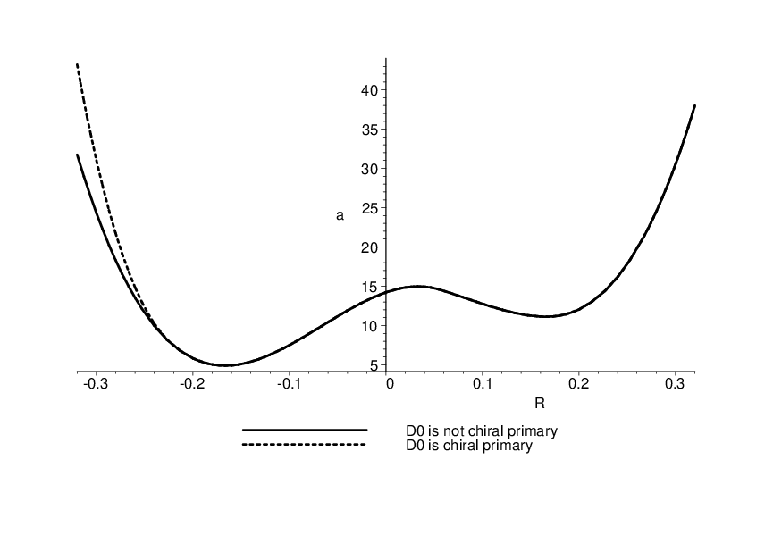
Strictly speaking, the $U(1)_{R}$ symmetry should be expressed as $U(1)_{R}=U(1)_{\lambda}+xU(1)_{F}+yU(1)_{M}$ instead of (4.1) at the local maximum because the $U(1)_{M}$ symmetry which transforms only $M^{ij}$ , appears at the infrared fixed point. Here, $y$ is determined so that the $U(1)_{R}$ charge of $M^{ij}$ becomes $2/3$ . However, the $U(1)_{R}$ charges of the other gauge invariant operators, except for that of the operator $M^{ij}$ , can be expressed as the sum of those of the component fields given by (4.30), because they have no charges under the $U(1)_{M}$ symmetry.

For $N_{Q}=8,9$ , as can be seen from Table 4.2, there are also five regions on the line of $R$ , as in Figure 4.3. As is different from the case of $N_{Q}=7$ , there is no region where the three gauge invariant operators $M$ , $Y$ , and $B$ hit the unitarity bounds at the same time, but a new region V, where only the operator $Y^{i}$ hits the unitarity bound, appears. Only for $N_{Q}=9$ , the operator $E$ is available, but it does not violate the unitarity bound over all the values of $R$ . If the spinor exotics $D_{1}$ are chiral primary in the infrared, our results for the regions I and II would be incomplete. The global trial $a$ -function $a(R)$ is similar to the one for $N_{Q}=7$ and have, in the region III, a single local maximum given by (4.30) with $N_{Q}=8,9$ substituted for each case, where also only the meson $M^{ij}$ is hitting the unitarity bound to be free in the infrared. This result does not depend on whether $D_{0}$ is chiral primary or not. The local maximum would be retained even after taking account of the exotics $D_{1}$ .

	Hitting Operators	Hitting Regions
I	$M$ , ( $D_{0}$ )	$R\leq-\frac{2}{9}$
II+III	$M$	$-\frac{2}{9}\leq R\leq\frac{1}{N_{Q}-1}(N_{Q}-\frac{20}{3})$
VI	$M$ , $Y$	$\frac{1}{N_{Q}-1}(N_{Q}-\frac{20}{3})\leq{R}\leq\frac{1}{3}$
V	$Y$	$\frac{1}{3}\leq R\leq\frac{1}{N_{Q}-5}(N_{Q}-\frac{20}{3})$
VI	$Y$ , $B$	$R\geq\frac{1}{N_{Q}-5}(N_{Q}-\frac{20}{3})$

Table 4.2: The five regions of the

U(1)_{R}

charge

R

for

N_{Q}=8,9

Figure 4.3: The operators hitting the unitarity bounds for the theory with

N_{Q}=8

and

9

vectors. The arrows show the regions where the corresponding operators hit the unitarity bounds.

For $10\leq{N_{Q}}\leq 21$ , it is remarkable that there exists a region V with no gauge invariant operators hitting the unitarity bounds, as shown in Figure 4.4. The parameter space of $R$ is divided into seven regions, as can be seen from Table 4.3. The regions I and II could be incomplete due to the exotics $D_{1}$ . The global trial $a$ -function $a(R)$ has a profile similar to the one in Figure 4.2. One finds the unique local maximum at

	$\displaystyle R(Q)=\frac{3N_{Q}^{2}-24N_{Q}-15+\sqrt{2885-N_{Q}^{2}}}{3(N_{Q}^{2}-5)},$		(4.31)
	$\displaystyle R(\Psi)=\frac{6N_{Q}^{2}+90-N_{Q}\sqrt{2885-N_{Q}^{2}}}{6(N_{Q}^{2}-5)}$		(4.32)

in the region V, where no operator hits the unitarity bound. The local maximum also remains valid even after taking account of the unitarity bound of $D_{1}$ .

	Hitting Operators	Hitting Regions
I	$M$ , $D_{2}$ , ( $D_{0}$ )	$R\leq-\frac{2}{9}$
II+III	$M$ , $D_{2}$	$-\frac{2}{9}\leq R\leq\frac{1}{15}$
IV	$M$	$\frac{1}{15}\leq R\leq\frac{1}{3}$
V	no operators	$\frac{1}{3}\leq R\leq\frac{1}{N_{Q}-1}(N_{Q}-\frac{20}{3})$
VI	$Y$	$\frac{1}{N_{Q}-1}(N_{Q}-\frac{20}{3})\leq R\leq\frac{1}{N_{Q}-5}(N_{Q}-\frac{20}{3})$
VII	$Y$ , $B$	$\frac{1}{N_{Q}-5}(N_{Q}-\frac{20}{3})\leq R\leq\frac{1}{N_{Q}-9}(N_{Q}-\frac{20}{3})$
VIII	$Y$ , $B$ , $E$	$R\geq\frac{1}{N_{Q}-9}(N_{Q}-\frac{20}{3})$

Table 4.3: The seven regions on the line of the

U(1)_{R}

charge

R

for

10\leq{N_{Q}}\leq 21

Figure 4.4: The operators hitting the unitarity bounds for the theory with

10\leq N_{Q}\leq 21

vectors. The arrows show the regions where the corresponding operators hit the unitarity bounds.

So far, we have determined the superconformal $U(1)_{R}$ charges of the gauge invariant chiral primary operators in the electric theory. One might wonder whether the same results could be obtained in the magnetic theory. Actually, this is automatically guaranteed by the ’t Hooft anomaly matching condition [35]. Since the magnetic theory saturates the anomalies of all the global symmetries of the electric theory [3, 4], the trial $a$ -function in the magnetic theory is identical to the one in the electric theory, even when the gauge invariant operators hit the unitarity bounds as long as the hitting operators are the same. By using (4.2) and Table 3.2, the $U(1)_{R}$ charges of the elementary fields of the magnetic theory can also be determined from the $U(1)_{R}$ charges of $Q$ or $\Psi$ determined above.

The $U(1)_{R}$ charges of the elementary fields of the electric theory and those of the magnetic theory are plotted in Figure 4.5 and 4.6. They indicate that the $U(1)_{R}$ charge of each elementary field is close to $2/3$ in the electric theory for large $N_{Q}$ and in the magnetic theory for small $N_{Q}$ . One therefore may regard that the electric theory and the magnetic theory are weakly interacting for large and small $N_{Q}$ , respectively, which is consistent with the conventional expectation.

In the one spinor case, we have found the unique local maximum of the trial $a$ -function for $10\leq{N_{Q}}\leq 21$ , where there are no gauge invariant chiral primary operators hitting the unitarity bounds. On the other hand, for $7\leq{N_{Q}}\leq 9$ , one also found the unique local maximum of the $a$ -function, but at the local maximum, one finds that the gauge invariant operator $M^{ij}$ is a free field at the infrared fixed point. Note that the existence of the local maximum is consistent with the conjecture [3, 4] that this theory is in the non-Abelian Coulomb phase for $7\leq{N_{Q}}\leq 21$ .

4.2 The Two Spinor Case

In this section, we will briefly give our results about a-maximization in the $Spin(10)$ theory with two spinors and $N_{Q}$ vectors for $6\leq N_{Q}\leq 19$ . Since our analysis of this case is quite similar to that in the previous section, we will not repeat a detailed explanation about it. See [15] for more details.

However, before proceeding, let us make a comment on two points, which is distinct from the one spinor case.

First, the magnetic theory has two gauge groups. From the one-loop beta functions of the two gauge couplings, one can see that the $SU(N_{Q}-3)$ gauge coupling is asymptotically free for $N_{Q}\geq 7$ , while the $Sp(1)$ coupling is asymptotically free for $N_{Q}\leq 7$ , perturbatively. Except for $N_{Q}=7$ , since there is no flavor number $N_{Q}$ where both of the gauge coupling constants are asymptotically free at the one-loop level, it might happen that either of the gauge interactions could be free at the infrared fixed point ³³ 3 The possibility will be discussed in detail in Chapter 6. . However, assuming below that both of the gauge interactions are not free at the infrared fixed point, $a$ -maximization will be carried out in the magnetic theory.

Second, as was discussed in the previous chapter, the classical chiral ring of the electric theory is not identical to the one of the magnetic theory. Therefore, at some values of the trial $U(1)_{R}$ charges, the set of the gauge invariant operators hitting the unitarity bounds in the electric theory is different from the one in the magnetic theory, which prevents us from finding the unique and correct trial $a$ -function. This problem is parallel to the problem concerning with the operator $D_{0}$ in the one spinor case. However, there are more extra operators as in (3.60) compared to the one spinor case, and, depending on whether each of them is chiral primary or not, there are many possibilities to consider, if we will use the same strategy as in the one spinor case. It is formidable for us to carry out the method of $a$ -maximization for each of all the possibilities. Therefore, we will pick up two of them; the case that all the extra operators in (3.60) are not chiral primary - the classical chiral ring of the electric theory - and the other case that they are all chiral primary - the classical chiral ring of the magnetic theory. Thus, we will carry out the $a$ -maximization procedure for the electric theory and the magnetic theory with their distinct classical chiral primary operators. Although we will implement the method of $a$ -maximization with the different global trial $a$ -function in the electric theory from the one in the magnetic theory, it will turn out that both the global trial $a$ -functions have the identical local maximum, which is consistent with the duality conjecture [7].

4.2.1 On the Electric Side

Let us begin with the electric theory. Similarly to the one spinor case, the trial $U(1)_{R}$ charges of the matter fields may be given by

\displaystyle R(Q)=-4x+1,\qquad R(\Psi)=N_{Q}x-1,

(4.33)

with the trial $U(1)_{R}$ symmetry given by a linear combination of $U(1)_{F}$ and $U(1)_{\lambda}$ in Table 3.4 as

\displaystyle U(1)_{R}=xU(1)_{F}+U(1)_{\lambda}

(4.34)

with a real number $x$ , assuming that there are no accidental global $U(1)$ symmetries ⁴⁴ 4 See the footnote 1 in this chapter. in the infrared.

For $N_{Q}=6$ , as can be seen from Figure 3.2, all the gauge invariant operators are $M$ , $Y$ , $C$ , $B$ , $G$ , $H$ , $D_{0}$ , and $S$ in (3.29). The $U(1)_{R}$ charges of the gauge invariant operators can be written in terms of $x$ as ⁵⁵ 5 Since the glueball $S$ of the $U(1)_{R}$ charge 2 never hits the unitarity bound, we will not take account of $S$ .

	$\displaystyle R(M)=-8x+2,\quad R(Y)=8x-1,\quad R(C)=1,\quad R(B)=-8x+3,$		(4.35)
	$\displaystyle R(G)=24x-4,\quad R(H)=8x,\quad R(D_{0})=-24x+8,$		(4.36)

as can be seen from Table 3.6. Their unitarity bounds divide all the values of $x$ into seven regions, as in Figure 4.7 ⁶⁶ 6 Since the operator $C$ does not hit the unitarity bound for any value of $x$ , it does not appear in the figure. .

The global trial $a$ -function is given by

\displaystyle a(x)=\left\{\begin{array}[]{ll}a_{0}(x)+f_{Y}(x)+f_{G}(x)+f_{H}(x),&\left(x\leq\frac{1}{12}\right)\cr\cr a_{0}(x)+f_{Y}(x)+f_{G}(x),&\left(\frac{1}{12}\leq x\leq\frac{1}{6}\right)\cr\cr a_{0}(x)+f_{M}(x)+f_{Y}(x)+f_{G}(x),&\left(\frac{1}{6}\leq x\leq\frac{7}{36}\right)\cr\cr a_{0}(x)+f_{M}(x)+f_{Y}(x),&\left(\frac{7}{36}\leq x\leq\frac{5}{24}\right)\cr\cr a_{0}(x)+f_{M}(x),&\left(\frac{5}{24}\leq x\leq\frac{7}{24}\right)\cr\cr a_{0}(x)+f_{M}(x)+f_{B}(x),&\left(\frac{7}{24}\leq x\leq\frac{11}{36}\right)\cr\cr a_{0}(x)+f_{M}(x)+f_{B}(x)+f_{D_{0}}(R),&\left(\frac{11}{36}\leq x\right)\end{array}\right.

where $a_{0}(x)$ is the local trial $a$ -function with no operators hitting the unitarity bounds, and the function $f_{\cal O}$ is similarly defined to the one in (4.25). The function (4.2.1) has a unique local maximum at

\displaystyle x=\frac{18N_{Q}+6-\sqrt{-4N_{Q}^{3}+143N_{Q}^{2}-928N_{Q}+1824}}{6(N_{Q}^{2}+8N_{Q}-12)},

(4.51)

with $N_{Q}=6$ , where only the operator $M^{ij}$ hits the unitarity bound and is free at the infrared fixed point.

For $N_{Q}=7$ , one can also find that only $M^{ij}$ hits the unitarity bound at the local maximum (4.51).

For $N_{Q}=8$ , all the values of $x$ are divided as in Figure 4.8 ⁷⁷ 7 In this case, the subtlety arises in the region $x\leq 1/4$ due to the lack of our knowledge of $a$ -maximization for Lorentz spinor operators like $D_{1\alpha}$ . The unitarity bound for a gauge invariant Lorentz spinor is $R({\cal O})\geq 1$ [8]. Our strategy for the issue is exactly the same as in the one spinor case.. The global trial $a$ -function has a unique local maximum at

\displaystyle x=\frac{12N_{Q}-\sqrt{2900-N_{Q}^{2}}}{6(N_{Q}^{2}-20)},

(4.52)

where no operators hit the unitarity bounds.

For $9\leq N_{Q}\leq 19$ , a local maximum is found at (4.52), where no gauge invariant operators hit the unitary bounds.

4.2.2 On the Magnetic Side

Let us turn to the magnetic theory. For $N_{Q}=6$ , the gauge invariant operators are $U_{0}$ , $U_{1}$ , $U_{2}$ , $E_{0}$ , $I_{0}$ , $I_{1}$ , and $J_{1}$ in (3.60), which exist only in the magnetic theory, besides $M$ , $Y$ , $C$ , $B$ , $G$ , $H$ , $D_{0}$ , and $S$ in (3.44), with their trial $U(1)_{R}$ charges given by (4.36) and by

	$\displaystyle R(U_{0})=24x-2,\quad R(U_{1})=4,\quad R(U_{2})=-24x+10,\quad R(E_{0})=-8x+5,$		(4.53)
	$\displaystyle R(I_{0})=8x+2,\quad R(I_{1})=3,\quad R(J_{1})=16x.$		(4.54)

Their unitarity bounds are illustrated in Figure 4.9 ⁸⁸ 8 Since the operators $C$ , $U_{1}$ and $I_{1}$ do not hit the unitarity bounds for all the values of $x$ , they do not appear in Figure 4.9. The bold arrows correspond to the operators which exist only in the magnetic theory. The dotted arrows correspond to the Lorentz spinor operators, which we ignore as in the previous subsection. .

For the region $1/9\leq x\leq 7/18$ , where neither of the operators which exist only in the magnetic theory, hits the unitarity bound, the global trial $a$ -function should be the same as the one in the electric theory, the latter of which has a local maximum in the range. Therefore, the global trial a-function in magnetic theory has at least one local maximum at the same value of $x$ . One can also show that it has no local maximum outside the region $1/9\leq x\leq 7/18$ .

For $7\leq N_{Q}\leq 19$ , this is also the case. In the magnetic theory, we obtain the same local maximum as in the electric theory, and there is no other local maximum of the global trial $a$ -function.

Chapter 5 Discussions

We have seen so far that the meson $M^{ij}=Q^{i}Q^{j}$ has no interactions for $7\leq{N_{Q}}\leq 9$ in the one spinor case and for $6\leq{N_{Q}}\leq 7$ in the two spinor case at the infrared fixed point. In this chapter, by using the electric-magnetic duality [3, 4, 7], we will give more elaborate discussions about what actually happens in the infrared when the meson becomes free.

The meson operator $Q^{i}Q^{j}$ in the electric theory corresponds to the elementary singlet $M^{ij}$ in the magnetic theory. For $7\leq{N_{Q}}\leq 9$ in the one spinor case, the singlet $M^{ij}$ becomes free at the infrared fixed point. Therefore, the coupling constant of the interaction term $M^{ij}\bar{q}_{i}\,s\,\bar{q}_{j}$ in the magnetic superpotential (3.9) must vanish at the point. It means that the interaction term should be irrelevant at the infrared fixed point. Since we now know the exact superconformal $U(1)_{R}$ charges of the chiral primary operators at the same point, and thus the exact conformal dimensions of them, we can precisely determine whether the interaction term $M^{ij}\bar{q}_{i}\,s\,\bar{q}_{j}$ is irrelevant or not at the fixed point.

In fact, taking account of the charge assignments in Table 3.2, one can see that the $U(1)_{R}$ charge of $\bar{q}_{i}\,s\,\bar{q}_{j}$ is $4x$ , and at the infrared fixed point, $R(\bar{q}_{i}\,s\,\bar{q}_{j})>4/3$ . Since the free meson operator $M^{ij}$ has the $U(1)_{R}$ charge $2/3$ , the $U(1)_{R}$ charge of the interaction term $M^{ij}\bar{q}_{i}\,s\,\bar{q}_{j}$ is greater than 2. Therefore, the interaction term is irrelevant at the infrared fixed point. This is consistent with the result that the meson $M^{ij}$ decouple from the remaining interacting system to be free in the infrared.

To the case $6\leq{N_{Q}}\leq 7$ with the two spinors, the same argument can be applied to find that the interaction terms of the meson $M^{ij}$ in the magnetic superpotential is irrelevant at the infrared fixed point.

Furthermore, let us consider another implication of the irrelevant interaction term. Since the equation of motion gives

\frac{\partial}{\partial M^{ij}}W_{\rm mag}=\frac{\tilde{h}}{\tilde{\mu}^{2}}N_{ij}=0,

where $N_{ij}=\bar{q}_{i}\,s\,\bar{q}_{j}$ , if its coupling constant $\tilde{h}$ were not zero, the gauge invariant operators $N_{ij}$ would be redundant. This is indeed the case for $10\leq N_{Q}\leq 21$ with one spinor and for $8\leq N_{Q}\leq 19$ with two spinors. However, for $7\leq N_{Q}\leq 9$ with one spinor and $6\leq N_{Q}\leq 7$ with two spinors, since $\tilde{h}$ goes to zero¹¹ 1 For $N_{Q}=7$ , the coupling constant $\tilde{h}^{\prime\prime}$ of the additional interaction term (3.10) also goes to zero., the operators $N_{ij}$ do not have to be redundant. Therefore, $N_{ij}$ should be a new generator of the chiral ring in the magnetic theory.

Furthermore, the magnetic theory with vanishing $\tilde{h}$ in the superpotential is dual to the same $Spin(10)$ theory but with the superpotential

W_{\rm ele}=N_{ij}Q^{i}Q^{j},

with the gauge singlets $N_{ij}$ and the free singlets $M^{ij}$ , which was explained in section 3.1.1 for the theory with one spinor but it is also the case for the theory with two spinors, though we haven’t previously mentioned about the latter case. The singlets $N_{ij}$ can be identified with $\bar{q}_{i}\,s\,\bar{q}_{j}$ . Therefore, the magnetic theory of the original dual pair flows into the magnetic one of another dual pair at the infrared fixed point. It suggests that the original electric theory flows into the electric theory with the superpotential $W_{\rm ele}$ as illustrated in Figure 5.1.

In the electric theory with the superpotential $W_{\rm ele}$ , we can carry out the $a$ -maximization procedure in a similar way to what we have done in the previous sections. The values of the trial $U(1)_{R}$ charge where no gauge invariant operators hit the unitarity bounds in this theory is identical to the values where only the operators $M^{ij}$ hit the unitarity bound in the original electric theory. In the region of the trial $U(1)_{R}$ charge, the local trial $a$ -function can be calculated in terms of the fundamental fields in the ultraviolet in the former theory to give

a_{0}(R)+\frac{N_{Q}(N_{Q}+1)}{2}F[R(N)]+\frac{N_{Q}(N_{Q}+1)}{2}F_{0},

where $a_{0}(R)$ is given in (4.3), $F(x)$ is defined as $F(x)\equiv 3(x-1)^{3}-(x-1)$ , and $F_{0}$ is the contribution from the free singlets $M^{ij}$ . Since the function $F(x)$ satisfies the relation

\displaystyle F(x)+F(2-x)=0,

(5.1)

one notices that $F[R(N)]=-F[R(QQ)]$ and that the above $a$ -function is the same as the one in the identical region in the original electric theory. Since the latter $a$ -function are constructed via the prescription of [11], one finds that it is consistent with the electric-magnetic duality.

Figure 5.1: Two dual pairs flow to the identical IR fixed point.

The origin of the singlet field $N_{ij}$ can also be captured in the original electric theory by using the auxiliary field method. In the original theory, let us introduce the auxiliary fields $M^{ij}$ and the Lagrange multipliers $N_{ij}$ to turn on the superpotential

\displaystyle W=N_{ij}\left(Q^{i}Q^{j}-h\,M^{ij}\right),

(5.2)

with the parameter $h$ . It does not change the original theory at all, as far as $h$ is non-zero. The equations of motion give the constraints

\displaystyle Q^{i}Q^{j}=h\,M^{ij},\qquad hN_{ij}=0.

(5.3)

Substituting them into (5.2), one can return to the original theory.

One can conceive that when the meson operator hits the unitarity bound, the parameter $h$ goes to zero in the infrared, due to the consistency with the result that the singlet $M^{ij}$ becomes free in the magnetic theory. In this case, the first equation of motion in (5.3) gives $Q^{i}Q^{j}=0$ while the second one gives the trivial identity $0=0$ . It is consistent with the result that the composites $Q^{i}Q^{j}$ decouple from the interacting system in the original theory while the chiral primary operator $N_{ij}$ is gained. Here, the decoupled free meson operators correspond to $M^{ij}$ , which are not related with vectors $Q^{i}$ of the interacting system any more. Furthermore, when $h$ goes to zero, one obtains the superpotential $W_{\rm ele}$ of the other electric theory introduced in subsection 3.1.1. It means that the original electric theory flows into the other electric theory with $W_{\rm ele}$ and thus is consistent with the magnetic picture.

One may raise a question whether the auxiliary field method affects our results via $a$ -maximization in the last section, because we introduced the auxiliary fields $M^{ij}$ and the Lagrange multipliers $N_{ij}$ charged under $U(1)\times{U(1)_{R}}$ . This is however not the case, since as has been discussed in [12], the massive fields $M^{ij}$ and $N_{ij}$ do not contribute to the $a$ -function, due to (5.1). But, once the singlet $M^{ij}$ hits the unitarity bound, an accidental $U(1)_{M}$ symmetry appears to fix the $U(1)_{R}$ charge of $M^{ij}$ to $2/3$ . On the other hand, the singlets $N_{ij}$ are still interacting with the vectors $Q^{i}$ in the superpotential, and their $U(1)_{R}$ charge remains unchanged and contributes as $F[R(N_{ij})]=F[2-R(Q^{i}Q^{j})]=-F[2R(Q)]$ to the $a$ -function;

F[R(M)]+F[R(N)]\quad\Rightarrow\quad F(2/3)+F[2-R(Q^{i}Q^{j})]=-F[2R(Q)]+F_{0}.

One can thus see that it gives the identical procedure to what we have done when the meson $M^{ij}$ hits the unitarity bound. This discussion gives a strong support for the prescription (2.74) in section 2.3. A similar support for it have been given in [36], where ${\cal N}=1$ supersymmetric $SU(N)$ gauge theory with an antisymmetric tensor and antifundamentals was studied via $a$ -maximization.

Chapter 6 Summary and Outlook

In this article, by using the electric-magnetic duality and $a$ -maximization to study four-dimensional supersymmetric ${\cal N}=1$ $Spin(10)$ gauge theories with chiral superfields in the vector and the spinor representations at the superconformal infrared fixed point, we have discussed their low-energy physics. In particular, $a$ -maximization allowed us to understand it in more detail, compared to the previous results [3, 4, 7] on the theories.

In the one spinor case, among $7\leq{N}_{Q}\leq 21$ in the non-Abelian Coulomb phase, for $7\leq{N}_{Q}\leq 9$ , only the meson operator hits the unitarity bound to be free in the infrared. For the other flavor number $N_{Q}$ , no gauge invariant operators hit the unitarity bound.

In the two spinor case, the results are quite parallel to that in the one spinor case. Among $6\leq{N}_{Q}\leq 19$ in the non-Abelian Coulomb phase, for ${N}_{Q}=6,7$ , only the meson operator also hits the unitarity bound to be free in the infrared. For the other flavor number $N_{Q}$ , no gauge invariant operators hit the unitarity bound.

In both the cases, the local maximum we found was confirmed to be identical in both of the electric theory and the magnetic theory.

We have also discussed the physical implication of the decoupling meson operator - the renormalization flows of two electric-magnetic dual pairs into a single nontrivial infrared fixed point - by the three steps; calculating the conformal dimension of the interaction term of the meson in the magnetic superpotential, finding another electric-magnetic dual pair, and using the auxiliary field method.

In our analysis, two subtle points prevents us from completing the $a$ -maximization procedure for the $Spin(10)$ gauge theories, as discussed in detail. One of them is the mismatch of the classical chiral rings of the electric-magnetic dual pairs. It means that a gauge invariant operator does not have their counterpart in the dual description. Therefore, at the value of the trial $U(1)_{R}$ charge where the operator hits the unitarity bound, the local trial $a$ -function differs from the one in the dual theory. Thus, the $a$ -maximization procedure might give different results in the electric theory from the one in the magnetic theory. Fortunately, this was not the case for our theories. However, in order to implement our $a$ -maximization procedure completely, we need to understand the chiral ring of the dual theories quantum-mechanically. It would also help to establish the electric-magnetic duality itself of the $Spin(10)$ gauge theories completely,

As for the other subtle point, we need to know how to extend the method of $a$ -maximization for a Lorentz spinor operator, and also for an operator in any non-trivial representation of the Lorentz group. In our cases, the operator $D_{1\alpha}$ is such a operator. Again, fortunately, the local maximum of the trial $a$ -function is found to be outside the region where the operator $D_{1\alpha}$ hits the unitarity bound. But, it does not necessarily mean that there is no local maximum inside the region. Therefore, it would be interesting to know the extension of $a$ -maximization for the operator $D_{1\alpha}$ .

Besides the two subtleties, during the $a$ -maximization procedure in the two spinor case, we have assumed in the magnetic theory that the gauge coupling constants of the magnetic gauge groups $SU(N_{Q}-3)$ and $Sp(1)$ both have non-zero values at the infrared fixed point. However, from the one-loop beta functions of the two gauge couplings, one can see that $SU(N_{Q}-3)$ is asymptotically free for $N_{Q}\geq 7$ and $Sp(1)$ is asymptotically free for $N_{Q}\leq 7$ , perturbatively. Therefore, either of the gauge interactions could be free at the infrared fixed point. Thus, if the perturbation of both the interactions were reliable even in the infrared, the gauge coupling constant of $SU(N_{Q}-3)$ would vanish for $N_{Q}=6$ and that of $Sp(1)$ would vanish for $8\leq N_{Q}\leq 19$ at the fixed point. We will argue just below that the method of $a$ -maximization could also have been used to know whether this is the case or not. Although our results suggest that this is not the case, it may offer another enjoyable application of $a$ -maximization [36, 37, 38].

Let us suppose that, for $N_{Q}=6$ , the coupling constant $g_{SU}$ of the $SU(N_{Q}-3)$ gauge interaction goes to zero in the infrared. The NVSZ beta function [23] of the gauge coupling $g_{SU}$ is given by

\displaystyle\beta_{SU}(g_{SU},g_{Sp})=-\frac{g_{SU}^{3}}{16\pi^{2}}\frac{3(N_{Q}-3)-\sum_{i}T(\rho_{i})(1-\gamma_{i}(g_{SU},g_{Sp}))}{1-(N_{Q}-3)({g_{SU}^{2}}/{8\pi^{2}})},

(6.1)

where $\gamma_{i}$ is the anomalous dimension of the matter field labeled by $i$ and $T(\rho_{i})$ denotes the usual index of its representation $\rho_{i}$ . Under our assumption, in the infrared the beta function can be expanded in powers of the gauge coupling $g_{SU}$ as

\displaystyle\beta_{SU}(g_{SU},g_{Sp})=\beta_{0}(g_{Sp})g_{SU}^{3}+\beta_{1}(g_{Sp})g_{SU}^{5}+\cdots,

(6.2)

where

\displaystyle\beta_{0}(g_{Sp})=-\frac{1}{16\pi^{2}}\left[3(N_{Q}-3)-\sum_{i}T(\rho_{i})(1-\gamma_{i}(g_{SU}=0,g_{Sp}))\right].

(6.3)

Therefore, in order to reach the infrared fixed point $(g^{*}_{SU}=0,g^{*}_{Sp})$ , the beta function coefficient $\beta_{0}(g^{*}_{Sp})$ must be positive - the infrared fixed point $(g^{*}_{SU}=0,g^{*}_{Sp})$ must be an attractive point of the renormalization group flow.

It is generically difficult to calculate the beta function coefficient $\beta_{0}(g^{*}_{Sp})$ , especially when the gauge coupling $g^{*}_{Sp}$ cannot be treated perturbatively. However, the anomalous dimensions $\gamma_{i}(g^{*}_{SU}=0,g^{*}_{Sp})$ are related to the superconformal $U(1)_{R}$ charges via $\gamma_{i}(g^{*}_{SU}=0,g^{*}_{Sp})=3R_{i}-2$ as in (2.42). In order to obtain the superconformal $U(1)_{R}$ charges, one may set the gauge coupling $g_{SU}$ to zero at the ultraviolet cutoff and then carry out $a$ -maximization. If one can identify the infrared fixed point $(g^{*}_{SU}=0,g^{*}_{Sp})$ as one of the local maxima of the global trial $a$ -function, and if no gauge invariant composite operator hits the unitarity bound, one can determine the $U(1)_{R}$ charge $R_{i}$ of the elementary field, and thus the coefficient $\beta_{0}(g^{*}_{Sp})$ .

In order to determine the coefficient $\beta_{0}(g^{*}_{Sp})$ , let us begin with the magnetic theory for $N_{Q}=6$ with $g_{SU}=0$ - the $Sp(1)$ gauge theory. All the $Sp(1)$ gauge invariant chiral primary operators are $M$ , $Y$ , $\bar{q}$ , $q$ , $s$ , and the composites

\displaystyle\varepsilon_{\alpha\beta}\bar{q}^{\prime}{}_{a}{}^{\alpha I}\bar{q}^{\prime}{}_{b}{}^{\beta J},\quad\varepsilon_{\alpha\beta}\bar{q}^{\prime}{}_{a}{}^{\alpha I}t^{\beta J},\quad\varepsilon_{\alpha\beta}t^{\alpha I}t^{\beta J}.

(6.4)

Since we do not impose the anomaly free condition coming from the $SU(N_{Q}-3)$ gauge interaction for the global $U(1)$ symmetries, one has one extra global $U(1)$ symmetry, and thus the trial $a$ -function depends on two parameters. It seems formidable to obtain the global trial $a$ -function in the whole two-dimensional parameter space. But, we found at least one local maximum in the range where $M$ , $Y$ , and $\bar{q}$ hit the unitarity bounds. At the local maximum, the $U(1)_{R}$ charge of each field can numerically be read as follows:

\displaystyle\begin{array}[]{|c|c|c|c|c|c|c|}\hline\cr\bar{q}&\bar{q}^{\prime}&q&s&t&M&Y\\ \hline\cr 2/3&0.4858&0.9716&1.028&0.5426&2/3&2/3\\ \hline\cr\end{array}

Substituting the $U(1)_{R}$ charges in the above list into the coefficient

\displaystyle\beta_{0}(g^{*}_{Sp})=-\frac{3}{16\pi^{2}}\left[(N_{Q}-3)-\sum_{i}T(\rho_{i})(R_{i}-1)\right],

(6.8)

since one can see that $\left[(N_{Q}-3)-\sum_{i}T(\rho_{i})(R_{i}-1)\right]\simeq 1$ , the coefficient $\beta_{0}(g^{*}_{Sp})$ is negative - the infrared fixed point into which the theory with $g_{SU}\not=0$ at the cutoff never flows in the infrared.

If there was no more local maximum of the global trial $a$ -function, the above argument would prove our assumption about the gauge couplings. Therefore, it would be interesting to carry out the $a$ -maximization procedure completely in this system to confirm the assumption.

In the case where the gauge coupling $g_{Sp}$ goes to zero in the infrared instead, a similar discussion can be made for $8\leq N_{Q}\leq 19$ . The $SU(N_{Q}-3)$ gauge invariant operators are the elementary field $t$ and the composites

$\displaystyle A^{\alpha(IJK)}$	$\displaystyle=$	$\displaystyle q^{aX}(\sigma_{X}\sigma_{2})^{(IJ}\bar{q}^{\prime}{}_{a}{}^{\|\alpha\|K)},$
$\displaystyle(P_{1})^{\alpha}{}_{i_{1}\cdots i_{N_{Q}-4}}$	$\displaystyle=$	$\displaystyle\varepsilon^{a_{1}\cdots a_{N_{Q}-3}}\bar{q}^{\prime}{}_{a_{1}}{}^{\alpha I}\bar{q}_{a_{2}i_{1}}\cdots\bar{q}_{a_{N_{Q}-3}i_{N_{Q}-4}},$
$\displaystyle(P_{3})^{\alpha}{}_{i_{1}\cdots i_{N_{Q}-6}}$	$\displaystyle=$	$\displaystyle\varepsilon^{a_{1}\cdots a_{N_{Q}-3}}\bar{q}^{\prime}{}_{a_{1}}{}^{\alpha_{1}I_{1}}\cdots\bar{q}^{\prime}{}_{a_{3}}{}^{\alpha_{3}I_{3}}\bar{q}_{a_{4}i_{1}}\cdots\bar{q}_{a_{N_{Q}-3}i_{N_{Q}-6}},$	(6.9)

as well as the operators which are the same as $SU(N_{Q}-3)\times Sp(1)$ gauge invariant operators except for $H$ and $G$ , which can be expressed in this case as the product of $SU(N_{Q}-3)$ gauge invariant operators.

We also found the local maximum of the trial $a$ -function; for $N_{Q}=8$ , in the range where $M$ and $t$ hit the unitarity bounds, for $N_{Q}=9$ , where $t$ hits the unitarity bound, and for $10\leq N_{Q}\leq 19$ , no operator hits the unitarity bound. The $U(1)_{R}$ charges of the fields are given in Table 6.1. Using the $U(1)_{R}$ charges, one can see that the NSVZ beta function becomes negative for all $8\leq N_{Q}\leq 19$ . It implies that the system does not flow in the infrared into the point which the above local maximum suggests. Since the analysis of $a$ -maximization in this case also is far from complete, it would be interesting to be done thoroughly.

$N_{Q}$	8	9	10	11	12	13	14	15	16	17	18	19
$\bar{q}$	0.516	0.482	0.462	0.440	0.417	0.396	0.376	0.357	0.339	0.323	0.308	0.295
$\bar{q}^{\prime}$	0.8	0.833	0.857	0.876	0.891	0.902	0.911	0.919	0.925	0.931	0.935	0.939
$q$	0.623	0.555	0.462	0.395	0.341	0.297	0.262	0.233	0.208	0.187	0.169	0.154
$s$	0.4	0.333	0.285	0.248	0.219	0.196	0.178	0.162	0.150	0.139	0.129	0.121
$t$	2/3	2/3	0.680	0.729	0.769	0.801	0.827	0.849	0.867	0.882	0.895	0.907
$M$	2/3	0.704	0.791	0.873	0.946	1.012	1.071	1.124	1.171	1.214	1.254	1.289
$Y$	0.861	0.963	1.076	1.166	1.242	1.307	1.362	1.411	1.453	1.490	1.522	1.551

Table 6.1: The

U(1)_{R}

charges under the assumption that the

Sp(1)

gauge interaction is IR free.

In our analysis, the trial $a$ -function has a unique local maximum under the assumptions mentioned above. Within a region with the same content of decoupling gauge invariant operators in the whole parameter space, one can find at most a single local maximum, but in another region, one could obtain another local maximum, where one should find the different content of interacting gauge invariant operators. It may suggest that one could find more than one local maximum over the whole parameter space to lose definitive results on which linear combination of the $U(1)$ symmetries is the superconformal $U(1)_{R}$ symmetry. The weak version of the diagnostic in the paper [33] could however be a way out of this problem. It says, “the correct IR phase is the one with the larger value of the conformal anomaly $a$ ”. It would thus be very interesting to find models with more than one local maximum of the function $a(x)$ and to study the renormalization group flow in such models.

Acknowledgments

We thank Yutaka Ookouchi and Yuji Tachikawa for collaborations and useful discussions. The work of T. K. was supported in part by a Grant-in-Aid (#19540268) from the MEXT of Japan. F. Y. is supported by the William Hodge Fellowship.

Bibliography

[1] I. Affleck, M. Dine and N. Seiberg, “Exponential Hierarchy from Dynamical Supersymmetry Breaking,” Phys. Lett. B 140 (1984) 59.
[2] H. Murayama, “Studying Non-calculable Models of Dynamical Supersymmetry Breaking,” Phys. Lett. B 355 (1995) 187, hep-th/9505082.
[3] P. Pouliot and M. J. Strassler, “Duality and Dynamical Supersymmetry Breaking in $Spin(10)$ with a Spinor,” Phys. Lett. B 375 (1996) 175, hep-th/9602031.
[4] T. Kawano, “Duality of ${\cal N}=1$ Supersymmetric $SO(10)$ Gauge Theory with Matter in the Spinorial Representation,” Prog. Theor. Phys. 95 (1996) 963, hep-th/9602035.
[5] P. Pouliot, “Chiral Duals of Nonchiral SUSY Gauge Theories,” Phys. Lett. B 359 (1995) 108, hep-th/9507018.
[6] P. Pouliot and M. J. Strassler, “A Chiral $SU(N)$ Gauge Theory and its Non-Chiral $Spin(8)$ Dual,” Phys. Lett. B 370 (1996) 76, hep-th/9510228.
[7] M. Berkooz, P. L. Cho, P. Kraus and M. J. Strassler, “Dual Descriptions of $SO(10)$ SUSY Gauge Theories with Arbitrary Numbers of Spinors and Vectors,” Phys. Rev. D 56 (1997) 7166, hep-th/9705003.
[8] G. Mack, “All Unitary Ray Representations of the Conformal Group $SU(2,2$ ) with Positive Energy,” Commun. Math. Phys. 55 (1977) 1.
[9] N. Seiberg, “Electric-Magnetic Duality in Supersymmetric Non-Abelian Gauge Theories,” Nucl. Phys. B 435 (1995) 129, hep-th/9411149.
[10] D. Kutasov and A. Schwimmer, “On Duality in Supersymmetric Yang-Mills Theory,” Phys. Lett. B 354 (1995) 315, hep-th/9505004.
[11] D. Kutasov, A. Parnachev and D. A. Sahakyan, “Central Charges and $U(1)_{R}$ Symmetries in ${\cal N}=1$ Super Yang-Mills,” JHEP 0311 (2003) 013, hep-th/0308071.
[12] E. Barnes, K. A. Intriligator, B. Wecht and J. Wright, “Evidence for the Strongest Version of the $4d$ $a$ -Theorem, via $a$ -Maximization along RG Flows,” Nucl. Phys. B 702 (2004) 131, hep-th/0408156.
[13] K. A. Intriligator and B. Wecht, “The Exact Superconformal $R$ -Symmetry Maximizes $a$ ,” Nucl. Phys. B 667 (2003) 183, hep-th/0304128.
[14] T. Kawano, Y. Ookouchi, Y. Tachikawa and F. Yagi, “Pouliot Type Duality via $a$ -Maximization,” Nucl. Phys. B 735 (2006) 1, hep-th/0509230.
[15] T. Kawano and F. Yagi, “Supersymmetric ${\cal N}=1$ $Spin(10)$ Gauge Theory with Two Spinors via $a$ -Maximization,” Nucl. Phys. B 786 (2007) 135, arXiv:0705.4022.
[16] S. Minwalla, “Restrictions Imposed by Superconformal Invariance on Quantum Field Theories,” Adv. Theor. Math. Phys. 2 (1998) 781, hep-th/9712074.
[17] F. A. Dolan and H. Osborn, “On Short and Semi-Short Representations for Four-Dimensional Superconformal Symmetry,” Annals Phys. 307 (2003) 41, hep-th/0209056.
[18] D. Anselmi, J. Erlich, D. Z. Freedman and A. A. Johansen, “Positivity Constraints on Anomalies in Supersymmetric Gauge Theories,” Phys. Rev. D 57 (1998) 7570, hep-th/9711035.
[19] D. Anselmi, D. Z. Freedman, M. T. Grisaru and A. A. Johansen, “Nonperturbative Formulas for Central Functions of Supersymmetric Gauge Theories,” Nucl. Phys. B 526 (1998) 543, hep-th/9708042.
[20] D. Poland and D. Simmons-Duffin, “Bounds on 4D Conformal and Superconformal Field Theories,” arXiv:1009.2087.
[21] R. Rattazzi, S. Rychkov and A. Vichi, “Central Charge Bounds in 4D Conformal Field Theory,” arXiv:1009.2725.
[22] R. Rattazzi, S. Rychkov and A. Vichi, “Bounds in 4D Conformal Field Theories with Global Symmetry,” arXiv:1009.5985.
[23] V. A. Novikov, M. A. Shifman, A. I. Vainshtein and V. I. Zakharov, “Exact Gell-Mann-Low Function of Supersymmetric Yang-Mills Theories from Instanton Calculus,” Nucl. Phys. B 229 (1983) 381.
[24] M. Chaichian, W. F. Chen and C. Montonen, “New Superconformal Field Theories in Four-Dimensions and ${\cal N}=1$ Duality,” Phys. Rept. 346, 89 (2001), hep-th/0007240.
[25] M. Flato and C. Fronsdal, “Representations of Conformal Supersymmetry,” Lett. Math. Phys. 8 (1984) 159.
[26] V. K. Dobrev and V. B. Petkova, “All Positive Energy Unitary Irreducible Representations of Extended Conformal Supersymmetry,” Phys. Lett. B 162 (1985) 127.
[27] F. Cachazo, M. R. Douglas, N. Seiberg and E. Witten, “Chiral Rings and Anomalies in Supersymmetric Gauge Theory,” JHEP 0212 (2002) 071, hep-th/0211170.
[28] N. Seiberg, “Adding Fundamental Matter to ’Chiral Rings and Anomalies in Supersymmetric Gauge Theory’,” JHEP 0301 (2003) 061, hep-th/0212225.
[29] A. B. Zamolodchikov, “Irreversibility of the Flux of the Renormalization Group in a $2D$ Field Theory,” JETP Lett. 43 (1986) 730, [Pisma Zh. Eksp. Teor. Fiz. 43 (1986) 565].
[30] J. L. Cardy, “Is There a $c$ -Theorem in Four Dimensions?,” Phys. Lett. B 215 (1988) 749.
[31] A. D. Shapere and Y. Tachikawa, “A Counterexample to the ‘ $a$ -Theorem’,” JHEP 0812 (2008) 020, arXiv:0809.3238.
[32] K. Intriligator, “Aspects of Supersymmetric Field Theories,” Int. J. Mod. Phys. A 25 (2010) 391.
[33] K. A. Intriligator, “IR Free or Interacting? A Proposed Diagnostic,” Nucl. Phys. B 730 (2005) 239, hep-th/0509085.
[34] C. Csaki, M. Schmaltz and W. Skiba, “Confinement in ${\cal N}=1$ SUSY Gauge Theories and Model Building Tools,” Phys. Rev. D 55 (1997) 7840, hep-th/9612207.
[35] G. ’t Hooft, “Naturalness, Chiral Symmetry, and Spontaneous Chiral Symmetry Breaking,” NATO Adv. Study Inst. Ser. B Phys. 59 (1980) 135.
[36] C. Csaki, P. Meade and J. Terning, “A Mixed Phase of SUSY Gauge Theories from $a$ -Maximization,” JHEP 0404 (2004) 040, hep-th/0403062.
[37] D. Poland, “The Phase Structure of Supersymmetric $Sp(2N_{c})$ Gauge Theories with an Adjoint,” JHEP 0911 (2009) 049, arXiv:0908.2131.
[38] D. Poland and D. Simmons-Duffin, “Superconformal Flavor Simplified,” JHEP 1005 (2010) 079, arXiv:0910.4585.

Chapter 1 Introduction

Chapter 2 𝒩=1{\cal N}=1 Superconformal Field Theory

2.1 𝒩=1{\cal N}=1 Superconformal Algebra

2.2 Central Charges in Four-Dimensional Conformal Field Theories

2.3 aa-Maximization

Chapter 3 S​p​i​n​(10)Spin(10) Theories and their Electric-Magnetic Duals

3.1 The Theory with One Spinor

3.1.1 Turning on a Superpotential

3.2 The Theory with Two Spinors

Chapter 4 The S​p​i​n​(10)Spin(10) Theories via aa-Maximization

4.1 The One Spinor Case

4.2 The Two Spinor Case

4.2.1 On the Electric Side

4.2.2 On the Magnetic Side

Chapter 5 Discussions

Chapter 6 Summary and Outlook

Bibliography

Chapter 2 ${\cal N}=1$ Superconformal Field Theory

2.1 ${\cal N}=1$ Superconformal Algebra

2.3 $a$ -Maximization

Chapter 3 $Spin(10)$ Theories and their Electric-Magnetic Duals

Chapter 4 The $Spin(10)$ Theories via $a$ -Maximization