As our understanding of theoretical high-energy physics has evolved, top-down considerations have motivated the exploration of “parallel sectors” comprised of their own particles and interactions but “hidden” from us (the visible sector) due to the weakness of the couplings connecting hidden and visible sector particles. In addition to providing new avenues for model-building, this broad framework opens up a range of exciting possibilities for the origin of Dark Matter (DM), which is the focus of this work. Understanding the origin of DM and its interactions within this framework is very important because experimental observations have only measured the gravitational effects of DM, leaving a large number of logical possibilities.

Assuming that the visible sector and other possible hidden sectors are initially in a state of thermal equilibrium, what are the possible production mechanisms for DM? If DM shares sizeable interactions with visible sector particles, then thermal equilibrium will be efficiently maintained until Freeze-Out (FO) renders a thermal relic abundance of DM via the standard WIMP paradigm [1]. Alternatively, it may be that DM couples extremely weakly to the visible sector and to itself, as is the case for so-called superWIMPs [2, 3] and FIMPs [4, 5]. A third and final possibility is that DM is very weakly coupled to the visible sector, but has substantial couplings to a hidden sector to which it is thermally equilibrated. In general, this hidden sector will contain its own set of particles and interactions and will have a temperature different from that of the visible sector¹¹ 1 If the temperature of the two sectors are the same, the sectors have equilibrated implying that there is only one sector.. The purpose of the present work is to systematically identify and characterize all possible origins of DM which might arise in this enormous class of theories.

We will assume throughout that DM is stable due to a symmetry shared by the visible and hidden sectors. Moreover, let us denote the lightest visible and hidden sector particles charged under this symmetry by $X$ and $X^{\prime}$, which have masses $m$ and $m^{\prime}$ taken to be broadly of order the weak scale such that $m>m^{\prime}$. By definition, $X^{\prime}$ is the DM particle. We also assume the existence of a weak coupling which bridges the visible and hidden sector and mediates the decay

where the ellipses denote what are typically visible decay products.

Remarkably, the cosmological evolution of this setup is entirely fixed by only a handful of parameters. This is analogous to standard single sector FO, where the DM abundance is solely determined by the DM annihilation cross-section. Here we find that DM relic abundance is fixed by following set of parameters in general:

where $\langle\sigma v\rangle$ and $\langle\sigma v\rangle^{\prime}$ are the thermally averaged annihilation cross-sections for $X$ and $X^{\prime}$, respectively, $\xi$ is the ratio of the visible and hidden sector temperatures, $\tau$ is the lifetime of $X$, and $\epsilon$ is a measure of the CP-phase in $X$ decays. In particular cases, the relic abundance depends on only a subset of the above parameters, as will be shown below.

We have evolved the cosmological history of the visible and hidden sectors over the parameter space defined in Eq. (2) in order to systematically identify all possible origins of hidden sector DM. Of course, the simplest possibility is that DM undergoes hidden sector Freeze-Out (FO^′), yielding a thermal relic abundance. This has been considered in many hidden sector models, and was studied systematically in [6]. On the other hand, the remaining possibilities for the origin of DM fall into two very broad categories:

• •

  Freeze-Out and Decay (FO&D). $X$ undergoes FO and then decays out of equilibrium, yielding an abundance of $X^{\prime}$. As we will see later, the final abundance of $X^{\prime}$ goes as

  $\displaystyle\Omega$

  $\displaystyle\propto$

  $\displaystyle\frac{m^{\prime}}{m\langle\sigma v\rangle}.$

  (3)

• •

  Freeze-In (FI). $X$ decays while still in thermal equilibrium with the visible sector, yielding an abundance of $X^{\prime}$. As we will see later, the final abundance of $X^{\prime}$ goes as

  $\displaystyle\Omega$

  $\displaystyle\propto$

  $\displaystyle\frac{m^{\prime}}{m^{2}\tau}.$

  (4)

Within the categories of FO&D and FI exist a number of distinct variations. For example, if FO&D or FI happen to produce an abundance of $X^{\prime}$ particles exceeding a particular critical value, then the $X^{\prime}$ particles will promptly undergo an era of “re-annihilation.” During this time the $X^{\prime}$ particles will efficiently annihilate within a Hubble time despite the fact that $X^{\prime}$ is no longer thermally equilibrated with the hidden sector. Because the final DM abundance changes accordingly, we refer to this mechanism of DM production as FO&D_r and FI_r. Another variation arises if $X$ decays are CP-violating, in which case FO&D and FI may produce an abundance of DM endowed with a particle anti-particle asymmetry. Such an effect is possible because although the visible and hidden sectors are separately in thermal equilibrium, they are not in equilibrium with each other. We denote these asymmetric modes of DM production by Asymmetric Freeze-Out and Decay (FO&D_a) and Asymmetric Freeze-In (FI_a). Note that these mechanisms are entirely distinct from the framework of Asymmetric DM [7], in which the DM particle anti-particle asymmetry is inherited from an already existent baryon asymmetry.

Crucially, as seen in Eqs. 3 and 4, each of these DM production mechanisms maps to a rather distinctive window in the parameter space spanned by $\tau$ and $\langle\sigma v\rangle$—and where all other parameters, $m$, $m^{\prime}$, $\langle\sigma v\rangle^{\prime}$, $\xi$, and $\epsilon$, are scanned over an inclusive range of values. This is remarkable because $\tau$ and $\langle\sigma v\rangle$ can, in principle, be measured at the LHC—after all, they are attributes of $X$, which is a visible sector field! For example, see the left panel of Figure 1, where each point corresponds to $\Omega h^{2}=0.11$, and each color denotes the dominant mechanism of DM production at that particular point in parameter space. Even though all parameters but $\tau$ and $\langle\sigma v\rangle$ have been scanned over a generous range, one sees that FO&D corresponds to a narrow band in $\langle\sigma v\rangle$ while FI corresponds to a narrow band in $\tau$.

On the other hand, it is also very likely that $m$, and perhaps even $m^{\prime}$, might be measured at colliders, for instance if the visible decay products of $X\rightarrow X^{\prime}+\ldots$ can be used to kinematically reconstruct the event. In the event that $m$ and $m^{\prime}$ are indeed measured, the boundaries between DM production mechanisms in the $\tau-\langle\sigma v\rangle$ plane become even more distinct, as shown in the right panel of Figure 1.

Because each production mechanism lies in a distinctive region in the $\tau-\langle\sigma v\rangle$ plane, we are left with the tantalizing possiblity that the origin of DM might be successfully reconstructed at the LHC even in this much broader framework compared to that of standard single sector FO. The purpose of the present work, however, is to establish a comprehensive understanding of the structures depicted in Figure 1, leaving a more detailed collider study to a companion paper [8].

The outline of this paper is as follows. In Section 2 we present a broad overview of two-sector cosmology. We begin with an analysis of our setup in a decoupled limit in which the visible and hidden sectors couple only through gravitational interactions. We then introduce portal interactions, and present a detailed discussion of the FO&D and FI mechanisms of DM production. Afterwards, we go on to discuss the effects of “re-annihilation”, followed by an analysis of the thermal properties of the coupled two-sector system. In Section 3, we present a series of cosmological phase diagrams depicting the dominant production mechanisms for DM as a function of the parameter space. We go on to discuss how the boundaries in these phase diagrams change with various parameters. In Section 4 we present a discussion of DM production from particle anti-particle asymmetries, and we conclude in Section 5.

Our setup is comprised of a visible and hidden sector, each with sizeable self-interactions which serve to maintain thermal equilibrium in each sector at temperatures $T$ and $T^{\prime}$, respectively. We assume that these sectors couple to one other only through portal interactions which are extremely feeble, so these temperatures are not equal, i.e. $T\neq T^{\prime}$. To begin, we limit the present discussion as well as that of Sections 2.1 and 2.2 to the case in which the visible and hidden sectors are entirely decoupled but for gravitational effects. In Section 2.3 and onwards we introduce portal interactions connecting the visible and hidden sectors and study the significant impact of these couplings on the cosmological history.

Throughout, we assume that the visible and hidden sectors enjoy a symmetry, discrete or continuous, that keeps DM cosmologically stable. The lightest visible sector particle charged under this stabilizing symmetry is denoted by $X$, and likewise in the hidden sector, $X^{\prime}$, which we take to be lighter than $X$. In the limit in which the visible and hidden sectors are decoupled, $X$ and $X^{\prime}$ are, of course, simultaneously stable. However, as portal interactions are switched on, $X$ becomes unstable and decays with a width $\Gamma$ into particles which ultimately yield an $X^{\prime}$ in the final state. We will study the cosmological evolution of the number densities $n$ and $n^{\prime}$ of $X$ and $X^{\prime}$, which obey the coupled Boltzmann equations

where $n_{\rm eq}$ and $n^{\prime}_{\rm eq}$ are the thermal equilibrium abundances and it is understood that here $\Gamma$ is thermally averaged and we work in a regime in which the effects of the corresponding inverse decays are negligible. Here we take the thermally averaged annihilation cross-sections, $\langle\sigma v\rangle$ and $\langle\sigma v\rangle^{\prime}$, to be independent of temperature. A primary aim of this paper is to study the most general cosmological evolution which follows from these equations, subject only to the requirement that $\langle\sigma v\rangle$ and $\langle\sigma v\rangle^{\prime}$ are large enough that both $X$ and $X^{\prime}$ undergo freeze-out. Note that we take the masses of $X$ and $X^{\prime}$, $m$ and $m^{\prime}$, both to be broadly of order the weak scale.

The relative size of $T$ and $T^{\prime}$ can have a drastic impact on the cosmological history. To see why this is so, let us define the ratio of temperatures to be

If we assume the standard picture of slow-roll inflation, then the inflaton can, in principle, couple with different strengths to the visible and hidden sectors. As a consequence, the decay of the inflaton reheats each sector to a different temperature, corresponding to an initial condition for $\xi$ given by $\xi_{\rm inf}=T^{\prime}_{\rm inf}/T_{\rm inf}$, the ratio of temperatures in each sector immediately after the decay of the inflaton, which we take to be less than 1. Naively $\xi=\xi_{\rm inf}$ for all time. However, interactions between the sectors can change $\xi$ from $\xi_{\rm inf}$. For example, scatterings between the sectors which are generically dominated in the UV, can increase the high temperature value of $\xi$ to $\xi_{\rm UV}$, which is taken to be a free parameter. In addition, there can be IR contributions to $\xi$ as well. These contributions are discussed in more detail in Section 2.7.

Even ignoring interactions between the two sectors, $\xi$ actually varies as a function of temperature due to the separate conservation of the co-moving entropies, $S=g_{*S}T^{3}$ and $S^{\prime}=g^{\prime}_{*S}T^{\prime 3}$, in each sector. Specifically, this implies that $\xi$ varies as a function of temperature to the extent to which the numbers of degrees of freedom in the visible and hidden sectors vary with temperature:

where $g_{*S}(T)$ and $g^{\prime}_{*S}(T)$ are the number of relativistic degrees of freedom in the visible and hidden sectors, respectively, when the visible sector is at a temperature $T$. A change in $g_{*S}(T)$ or $g^{\prime}_{*S}(T)$ by an order of magnitude only affects $\xi$ at the level of a factor of two; hence, when comparing DM production from processes at different temperatures, this effect may be justifiably ignored.

In general, the energy density in the hidden sector affects the expansion rate of the universe during BBN, which places an important, albeit weak constraint on $\xi$. In particular, any hidden sector particles which are relativistic at BBN contribute an effective number of extra neutrino species

The present bound from experiment is $\Delta N_{\nu}<1.4$ [9], which is surprisingly mild: that is, for $g_{*}^{\prime}(T_{\rm BBN})=100$, this is satisfied by taking $\xi(T_{\rm BBN})=1/3$. Furthermore, according to Eq. (8), at higher temperatures $\xi$ can be close to unity even if $g^{\prime}_{*}>100$ [6].

A primary aim of this paper is to identify and characterize all possible mechanisms of DM production which can arise within our general two-sector framework. To this end, we have simulated the cosmological history of this system over a broad range of values for the relevant parameters:

where $\xi_{\rm UV}$ is the UV initial condition for $\xi$ which receives contributions from the decay of the inflaton as well as scattering processes from higher-dimensional operators described in Eq. (32)³³ 3 Here we also take $\xi_{\rm UV}$ to include effects from additional sources of entropy dumping into either sector before the weak era, so that $\xi_{\rm UV}$ is effectively the weak scale value of $\xi$, modulo the contribution from $X$ decays in the IR.. As noted earlier, it is quite remarkable that the cosmology is determined solely by just a handful of quantities.

In this section we present a series of “cosmological phase diagrams” depicting the regions in parameter space in which each mode of DM production, i.e. FO&D, FI, etc., accounts for the dominant contribution to the present day DM abundance. For example, Figure 7 is a cosmological phase diagram in the $\tau-\frac{\langle\sigma v\rangle^{\prime}}{\langle\sigma v\rangle}$ plane for particular values of $\{m,m^{\prime},\langle\sigma v\rangle,\xi_{\rm UV}\}$, as explained in the caption. Each colored shaded region corresponds to a particular DM production mode which is dominant in that region. The boundaries of each phase have been computed analytically. The solid black contours correspond to the present day DM relic abundance, calculated numerically using the coupled Boltzmann equations in Eqs. (5). Let us consider some of the features of Figure 7 in detail.

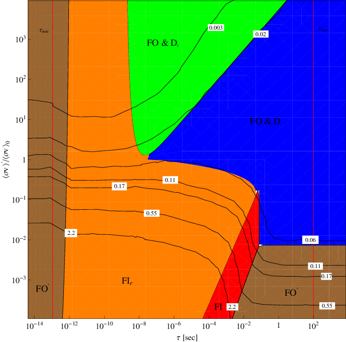
First, note that the lifetime $\tau$ is constrained both from above and below as shown by the red vertical lines in Figure 7. The upper limit is easy to understand as it originates from the requirement the decay products of $X$ do not ruin the successful predictions of BBN [13]. While the precise constraint depends on the nature of $X$ and its decay products, here we use

as depicted by the red line at large $\tau$ in Figure 7. The lower limit on $\tau$ comes from demanding that the two sectors are not in thermal equilibrium with each other at the weak scale. In Section 2.7 we found that for $\xi_{\rm UV}^{4}\ll 1$, the two sectors becomes thermally equilibrated if the lifetime is shorter than

For $\tau\lesssim 10^{-13}$ s, the two sectors are, from a cosmological perspective, a single sector. As a consequence, there is no distinction between FO and FO^′—the visible and hidden sectors together maintain thermal equilibrium until $X^{\prime}$ undergoes single sector FO^′. This is depicted by the brown region in the left in Figure 7. The yield $Y^{\prime}_{\textrm{FO}^{\prime}}$ in this region is independent of $\tau$ because $\xi_{\textrm{FO}^{\prime}}=1$ in the expression for $Y^{\prime}_{\textrm{FO}^{\prime}}$ in Table 1. Note that the brown region extends to $\tau$ larger than $\tau_{\rm min}$, as will be discussed soon.

Next, let us discuss the salient features of Figure 7 as we move from the largest to the smallest allowed values for $\tau$. Furthermore, for a given value of $\tau$, the dominant DM production mechanism changes as a function of $\frac{\langle\sigma v\rangle^{\prime}}{\langle\sigma v\rangle}$. For example, for the choice of parameters in Figure 7, one finds that FO&D and $\textrm{FO}^{\prime}$ dominate over FI for $10^{-1}\textrm{ s}\lesssim\tau\lesssim 100$ s. This is because the lifetime is too long (the coupling is too weak) for the FI mechanism to set in, as shown in Section 4. For values of $\tau$ in the above range with $\frac{\langle\sigma v\rangle^{\prime}}{\langle\sigma v\rangle}\gtrsim 10^{-1}$, corresponding to the blue shaded region, FO&D is the dominant mechanism. Indeed, from the shape of the contours one can see that in this region the relic abundance is independent of $\frac{\langle\sigma v\rangle^{\prime}}{\langle\sigma v\rangle}$ and $\tau$ as dictated by the expression for $Y^{\prime}_{{\rm FO\&D}}$ in Table 1. For $\frac{\langle\sigma v\rangle^{\prime}}{\langle\sigma v\rangle}\lesssim 10^{-2}$, $\textrm{FO}^{\prime}$ starts to dominate over FO&D since the annihilation cross-section of $X^{\prime}$ becomes sufficiently small. This is shown by the brown region in the right in the figure. For such long lifetimes, one finds that $\xi_{\textrm{FO}^{\prime}}\approx\xi_{\rm UV}$ from (32), implying that $Y^{\prime}_{\textrm{FO}^{\prime}}$ is essentially independent of $\tau$ (see the expression for $Y^{\prime}_{\textrm{FO}^{\prime}}$ in Table 1). Thus, the contour lines in this region are roughly horizontal. The boundary between the FO&D and $\textrm{FO}^{\prime}$ regions for this range of $\tau$ is given by :

which in the $\frac{\langle\sigma v\rangle^{\prime}}{\langle\sigma v\rangle}-\tau$ plane corresponds to $\frac{\langle\sigma v\rangle^{\prime}}{\langle\sigma v\rangle}\approx$ constant, since $\xi_{\textrm{FO}^{\prime}}\approx\xi_{\rm UV}$.

For $10^{-8}\textrm{ s}\lesssim\tau\lesssim 10^{-4}-10^{-1}$ s, FI and $\mathrm{FI_{r}}$ begin to dominate over FO&D and $\textrm{FO}^{\prime}$ because the portal interactions between sectors is growing stronger. In particular, FI is dominant in the narrow band shown by the red shaded region in Figure 7. For FI to be the dominant mechanism, the yield from FI must be larger than that from $\textrm{FO}^{\prime}$ but smaller than that from ${\rm FI}_{r}$; hence the narrow band in which FI is the dominant mechanism. The boundary curves between the ${\rm FI}$ region and the $\textrm{FO}^{\prime}$ $\&$ ${\rm FI}_{r}$ regions are given by:

Both curves imply a linear relation between $\frac{\langle\sigma v\rangle^{\prime}}{\langle\sigma v\rangle}$ and $\tau$, only with different coefficients⁴⁴ 4 The boundary shown in Eq. (52) depends on $\xi_{\textrm{FO}^{\prime}}$ as well, but in this region $\xi_{\textrm{FO}^{\prime}}\approx\xi_{\rm UV}$ is a constant.. Also, note from Table 1 that $Y^{\prime}_{{\rm FI}}$ does not depend on $\frac{\langle\sigma v\rangle^{\prime}}{\langle\sigma v\rangle}$, hence the contour lines for the relic abundance are almost vertical. They are not completely vertical since it turns out that ${\rm FI}$ never fully dominates the contribution to the relic abundance.

For $10^{-8}\textrm{ s}\lesssim\tau\lesssim 10^{-4}-10^{-1}$ s with $\frac{\langle\sigma v\rangle^{\prime}}{\langle\sigma v\rangle}\lesssim 1$, the FI yield becomes so large that it exceeds the critical yield at $T_{{\rm FI}_{r}}$, implying that $X^{\prime}$ starts to re-annihilate and the yield is given by $Y^{\prime}_{{\rm FI}_{r}}$. This is shown by the orange region in the figure. From Table 1, one sees that contours for $Y^{\prime}_{{\rm FI}_{r}}$ are essentially horizontal since the dependence on $\tau$ only arises from the logarithm. As one increases $\frac{\langle\sigma v\rangle^{\prime}}{\langle\sigma v\rangle}$ above roughly unity, FO&D starts to dominate over ${\rm FI}_{r}$ as shown by the blue region, since the annihilation cross-section of $X^{\prime}$ becomes large enough that the yield $Y^{\prime}_{{\rm FI}_{r}}$ becomes smaller than $Y^{\prime}_{\mathrm{FO\&D}}$. The boundary curve between these two regions is defined by:

showing that $\frac{\langle\sigma v\rangle^{\prime}}{\langle\sigma v\rangle}$ is essentially constant up to a logarithmic dependence.

If $\frac{\langle\sigma v\rangle^{\prime}}{\langle\sigma v\rangle}$ is further increased, FO&D is eventually superseded by $\mathrm{FO\&D_{r}}$ as shown by the green region. In this case the $X^{\prime}$ yield from the freezeout and decay of $X$ is so large that it becomes larger than the critical yield; so $X^{\prime}$ starts re-annihilating with a yield given by $Y^{\prime}_{\mathrm{FO\&D}_{r}}$. From Table 1, the contour plots for $Y^{\prime}_{\mathrm{FO\&D}_{r}}$ follow a simple power law ($\frac{\langle\sigma v\rangle^{\prime}}{\langle\sigma v\rangle}\propto\sqrt{\tau}$). The boundary curve between the FO&D and ${\rm FO\&D_{r}}$ regions is given by:

showing that the boundary also follows the same power law as the DM yield contours.

For ${\rm few}\times 10^{-13}\textrm{ s}\lesssim\tau\lesssim 10^{-8}$ s, ${\rm FI}_{r}$ is again the dominant mechanism as shown by the orange region. It dominates over $\mathrm{FO\&D_{r}}$ in particular, since the yield is inversely proportional to the relevant temperatures for $\mathrm{FO\&D_{r}}$ and ${\rm FI}_{r}$, which are $T_{{\rm FO\&D_{r}}}$ and $T_{{\rm FI}_{r}}$ respectively, and $T_{{\rm FO}_{r}}$ is larger for small lifetimes (large $\Gamma$) compared to $T_{{\rm FI}_{r}}$ from Table 1. The boundary curve between these two regions is given by:

References

- [1] E. W. Kolb and M. S. Turner, “The Early Universe.” (1988).
- [2] J. L. Feng, A. Rajaraman and F. Takayama, Phys. Rev. D 68, 063504 (2003) [arXiv:hep-ph/0306024].
- [3] J. L. Feng, S. f. Su and F. Takayama, Phys. Rev. D 70, 063514 (2004) [arXiv:hep-ph/0404198].
- [4] L. J. Hall, K. Jedamzik, J. March-Russell and S. M. West, JHEP 1003, 080 (2010) [arXiv:0911.1120 [hep-ph]].
- [5] T. Asaka, K. Ishiwata and T. Moroi, Phys. Rev. D 73, 051301 (2006) [arXiv:hep-ph/0512118].
- [6] J. L. Feng, H. Tu and H. B. Yu, JCAP 0810, 043 (2008) [arXiv:0808.2318 [hep-ph]].
- [7]
D. E. Kaplan, M. A. Luty and K. M. Zurek,
Phys. Rev. D 79, 115016 (2009)
[arXiv:0901.4117 [hep-ph]].
Y. Cai, M. A. Luty and D. E. Kaplan, arXiv:0909.5499 [hep-ph]. - [8] C. Cheung, G. Elor, L. J. Hall, P. Kumar, JHEP 1103, 085 (2011). [arXiv:1010.0024 [hep-ph]].
- [9] C. Amsler et al. [Particle Data Group], Phys. Lett. B 667, 1 (2008).
- [10] T. Asaka and T. Yanagida, Phys. Lett. B 494, 297 (2000) [arXiv:hep-ph/0006211].
- [11] C. Cheung, Y. Nomura and J. Thaler, JHEP 1003, 073 (2010) [arXiv:1002.1967 [hep-ph]].
- [12] C. Cheung, J. Mardon, Y. Nomura and J. Thaler, JHEP 1007, 035 (2010) [arXiv:1004.4637 [hep-ph]].
- [13] T. Moroi, H. Murayama and M. Yamaguchi, Phys. Lett. B 303, 289 (1993).
- [14] L. J. Hall, J. March-Russell and S. M. West, arXiv:1010.0245 [hep-ph].