Three Balls Problem Revisited – On the Limitations of Event-Driven Modeling
Abstract
If a tennis ball is held above a basket ball with their centers vertically aligned, and the balls are released to collide with the floor, the tennis ball may rebound at a surprisingly high speed. We show in this article that the simple textbook explanation of this effect is an oversimplification, even for the limit of perfectly elastic particles. Instead, there may occur a rather complex scenario including multiple collisions which may lead to a very different final velocity as compared with the velocity resulting from the oversimplified model.
pacs
45.70.-n,45.70.Qj,47.20.-kI Introduction
Consider a set of two balls made of the same viscoelastic material whose centers are vertically aligned at positions and as sketched in Fig. 1.
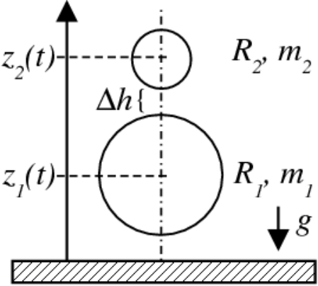
Let and be the radii of the particles and their initial vertical spacing. At time we release the particles to collide with the floor. The question for the maximum height reached by the upper sphere after the collision is then a common textbook problem. The textbook solution is based on the assumption that the collisions of the lower particle with the floor and the subsequent collision of the lower particle with the upper one are separate two-body interactions which may be treated independently, that is, one disregards the duration of the collisions. Whether this assumption is justified depends, of course, on the initial conditions, the particle sizes and the material parameters.
The experimental investigation of the described problem is tricky as even a small deviation from the vertical alignment of the initial positions of the spheres leads to considerable post-collisional velocities in horizontal direction, in particular, if more than two balls are involved. Simple but effective techniques were introduced[1, 2, 3], which allow for experiments with chains of up to about 7 aligned balls.
In this paper we will show that although the problem looks simple, there may emerge rather complex behavior including multiple collisions. The simple solution mentioned above is, thus, only a special case of a more general solution.
II Independent Collision Model
II.1 Collision Scenario
To introduce our notation and for later reference let us first reproduce the solution for the independent collisions model (ICM), that is, the final velocity of the upper ball is the result of a) the inelastic collision of the lower ball with the floor and b) the inelastic collision of the lower ball with the upper ball. Note that here and in the following we restrict ourselves to the situation where . For the opposite case, , it may be shown that the sketched sequence of collisions fails, even under the assumption of perfectly elastic collisions[1, 4].
Inelasticity of the balls is described by the coefficient of restitution which relates the precollisional relative velocity of colliding particles, and to the post-collisional one, ,
| (1) |
The lower sphere () reaches the floor at time at the velocity from where it is reflected with . The first index always denotes the considered particle and the second its collision-partner. Index 0 stands for the floor, 1 for the lower and 2 for the upper sphere. Upper index (0) stands for initial values. Post-collisional values are marked by primes. The particles collide then at whereby the upper sphere is located at position with the initial height . At the lower particle has the velocity and the upper . Employing the collision rule, Eq. (1), and conservation of momentum, we obtain the final velocities
| (2) | |||||
| (3) |
and the relative velocity
| (4) |
In the case of elastic () and instantaneous () collisions we find
| (5) | |||||
| (6) |
For the lower sphere loses all its kinetic energy () and the upper sphere rebounds with twice its initial velocity. In the limit we recover the well known textbook result , that is, the upper ball rises to about nine times of its initial dropheight ().
The system of bouncing balls can be exhaustively described also for more than two spheres [5], provided the collisions are considered as isolated events, that is, only two-particle interactions are taken into account.
II.2 Coefficient of Restitution Resulting from the Solution of Newton’s Equation
The contact of viscoelastic spheres is described by the (modified) Hertz contact law [6]. In this article we will use a simplified force law since it allows for a exhaustive analytical solution of the problem. To justify this approximation, we will show later by means of numerical simulations that the more correct Hertz contact force leads to qualitatively identical results, see Appendix B.
We describe the contact of dissipatively interacting particles, and , by
| (7) |
as a function of the mutual compression
| (8) |
and the compression rate , where is the radius of particle and is its position at time . The expression in square brackets in Eq. (7) may become positive during the expansion phase, that is, the (positive) dissipative force may overcompensate the (negative) elastic force which would lead to a resulting erroneous attractive force, see e.g. [7]. Therefore, the function is applied to take into account that the interaction force is always repulsive (negative).
Consider an isolated pair of colliding particles and approaching one another at impact rate at . Using the force, Eq. (7), we obtain the relative velocity after a collision by solving Newton’s equation of motion,
| (9) |
with the effective mass and initial conditions and . The collision is complete at time when [7].
Of course, for a pairwise collision the final velocity as obtained from Eq. (1) must coincide with the final velocity as obtained from integrating Newton’s equation of motion. Therefore, the solution of Eq. (9) allows to relate the coefficient of restitution to the parameters and of the force law, Eq. (7), via
| (10) |
Straightforward calculation [7] yields for the
duration of the collision
| (11) |
with
| (12) |
For the coefficient of restitution we obtain
| (13) |
where . Note that depends on the parameters of the force and the effective mass of the colliding particles, that is, . Thus, may not be considered as a pure material constant.
III Simultaneous Contacts
III.1 Equations of Motion
The ICM fails if we take into account the finite duration of the collisions. In this case, it may happen that the collision of the particles (process b) starts yet before the collision of the lower particle with the floor (process a) has terminated. In this case we have a three-particle interaction of the floor and both balls which cannot be resolved using the concept of the coefficient of restitution. In this case, the final velocity of the upper particle must be determined by integrating Newton’s equation of motion for the three-particle system which requires the detailed knowledge of the interaction forces. Consequently, we have to solve the set of Newton’s equations
| (14) |
where is the model-specific interaction law between particles and and the floor is considered as particle 0 (with ).
The failure of the simplifying ICM was discussed in the context of the closely related problem of Newton’s cradle. A simple analysis reveals immediately that the textbook-like explanation using isolated collisions is insufficient [8]. Instead, the details of the interaction force must be taken into account. The explanation of Newton’s cradle is far from being simple and there is an intensive and controversial discussion about this seemingly simple classroom experiment [9, 10, 11, 12, 13, 14, 15, 16].
The necessity of considering the details of the interaction force becomes obvious immediately when considering colliding rods instead of spheres [17, 18, 19]. In fact, the investigation of longitudinal waves in colliding bodies and the corresponding duration of the collision is a classical problem of mechanics, investigated by some of the most eminent scientists, such as Poisson [20], Boltzmann [21] and other important scientists [22, 23, 24]
III.2 Comparison with the ICM
In Sec. II.2 we conclude the coefficient of restitution from the interaction force. Using this result, we can compute the final relative velocity by means of Eq. (4), employing the assumption of independent collisions. Alternatively we can obtain by solving the set of equations (14) numerically. The latter approach does not require any assumption on the sequence of the collisions. We will see that both results may deviate considerably according to rather complex dynamics of the system.
In order to compare both results by means of Eq. (13) we map the constants of the force law to the coefficient of restitution .
We assume that the collisions between the lower sphere and the floor () and between the spheres () take place at the same coefficient of restitution. Since the effective mass enters Eq. (13), for given material stiffness, , Eq. (13) then provides a relation between and , thus, we can determine by specifying as a control parameter of the problem.
The latter assumption implies the somewhat unphysical fact that the lower side of the large sphere (where it contacts the floor) is characterized by a larger dissipative constant than its upper side (where it contacts the smaller sphere). We will justify this assumption in App. C where we show that the perhaps more plausible assumption , implying , leads to qualitatively identical results.
IV Basketball – Tennis Ball Problem
IV.1 Collision Sequence
Let us assume two vertically aligned balls (the basketball – tennis ball problem) as sketched in Fig. 1. We integrate Newton’s equation of motion, Eq. (14), for this system numerically and obtain the forces between the bottom and the lower sphere and between both spheres, see Fig. 2.
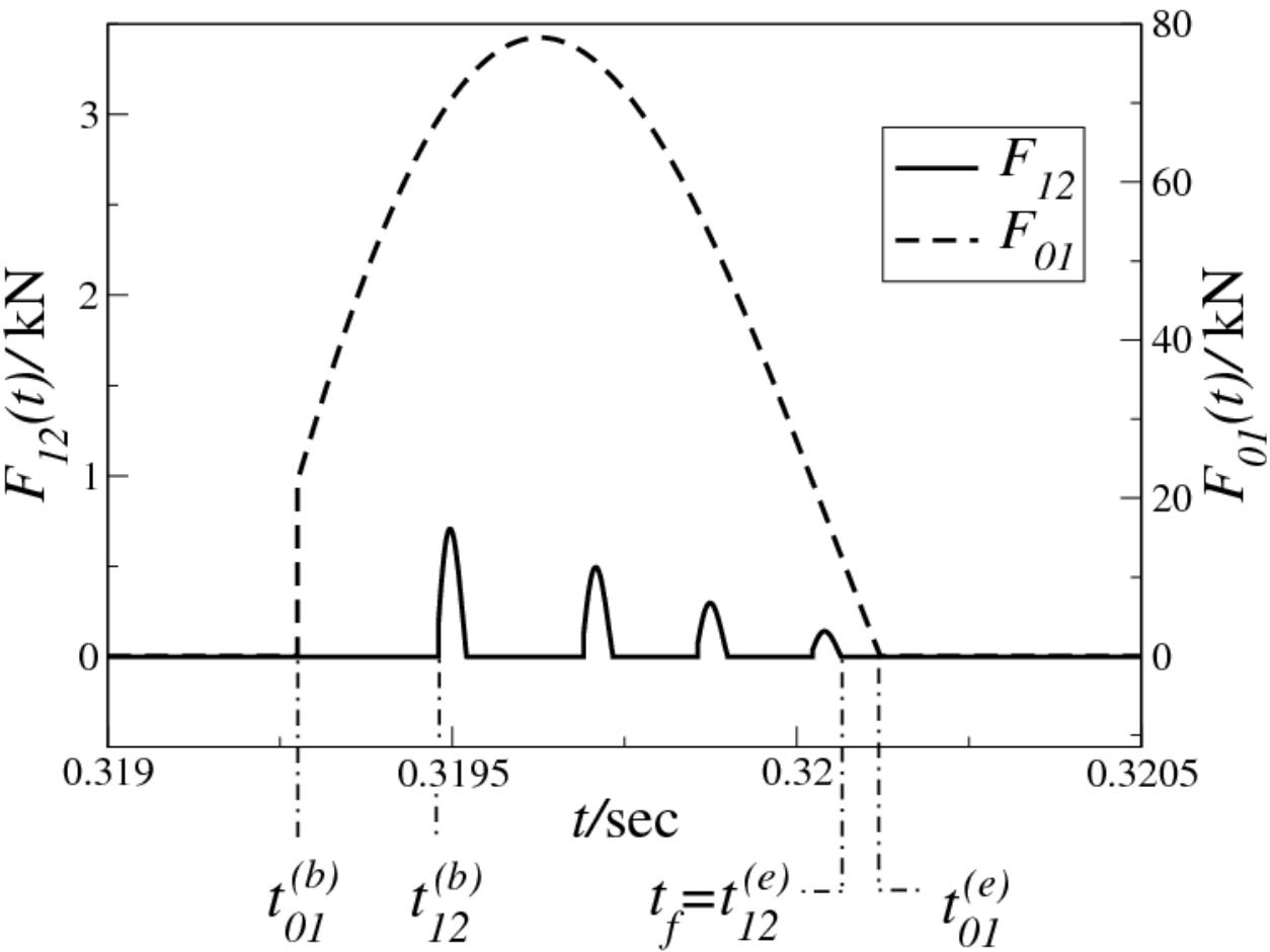
For time the lower particle is in contact with the floor as indicated by the force . During this interval the balls are in contact repeatedly, starting at time (first contact) and ending (last contact) at time as indicated by . An interesting detail is the discontuity of at which is a consequence of the force law, Eq. (7): At the instant of the contact where , the elastically restoring term, , vanishes whereas the (repulsive) dissipative term, , has a finite value as soon as the particles get into contact.
The existence of multiple collisions shown in Fig. 2 shows that the ICM described in Sec. II fails for the chosen set of parameters which provokes mainly two questions:
- 1.
How many contacts between the spheres occur and how does their number depend on the system parameters (, , , or respectively)?
- 2.
If multiple collisions take place, when does the collision sequence terminate?
Depending on the system parameters we may obtain or , therefore, the second question must be answered by a definition: The collision-sequence terminates at time (see Fig. 2) when the last contact between the spheres ceases, before the large sphere collides with the floor for the second time.
To answer the first question, we refer to Fig. 3 which illustrates the sequence of collisions in dependence of the coefficient of restitution for fixed and .
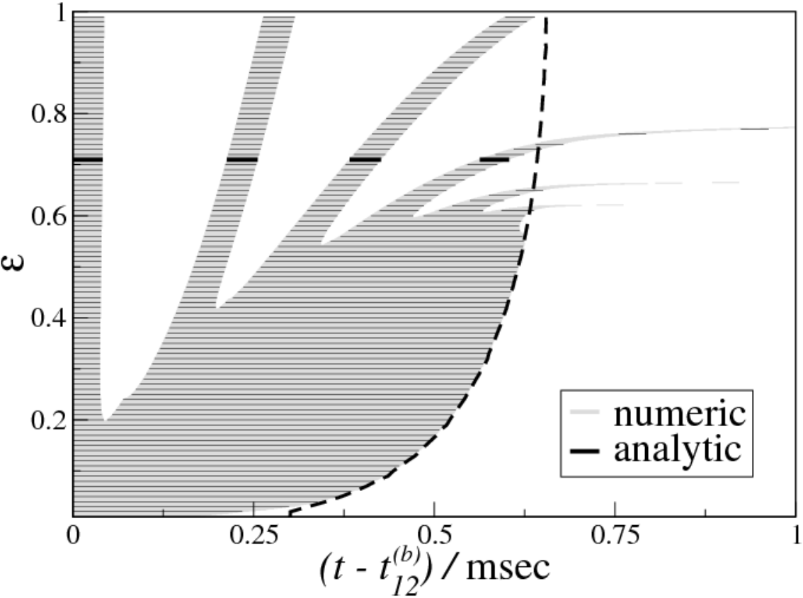
The value of was adjusted by varying , according to Eq. (13) while keeping invariant. Figure 3 should be read horizontally (for fixed value of ): each black or grey line marks time intervals when the particles are in contact. For elastic balls, , and the chosen parameters there occur 3 collisions. For sufficiently large , this number may be unity, that is, the independent-collisions condition is fulfilled (see below). Keeping , and the radii and constant and decreasing , the number of contacts increases. This is due to the fact that the relative velocity of the balls decreases because of inelastic collisions and, thus, the intervals of free flight become shorter while the duration of the contacts depends only weakly on the value of the inelasticity. For yet smaller the relative velocity after the contact may be small enough such that the lower ball catches up with the upper because of its upwards acceleration due to its contact with the floor. This effect makes some free-flight intervals vanish for decreasing and, thus, reduces the number of contacts. Summarizing, for each set of parameters , , , the number of collisions as a function of is a function with a single maximum.
For the force law Eq. (7) the basketball – tennis ball problem may be solved analytically by a piecewise procedure, see App. A. To check against numerical errors, the horizontal gray lines (in between the black lines) show the same information as the result of an analytical theory which agrees perfectly with the numerical data.
There is an interesting case when the final velocity of the lower ball after losing contact with the floor is only slightly larger than the velocity of the upper ball after the previous collision. Since both balls move only under the action of gravity, the balls may collide an ultimate time even after the contact between the lower ball and the floor has already finished. These events may be seen in Fig. 3 as narrow spikes at , , etc.
The number of contacts of the spheres as a function of and the initial distance is shown in more detail in Figure 4 (top). As explained above for each value of there is an interval for which maximizes the number of contacts.


For the interaction force, Eq. (7) the ratio of the contact duration of the collision lower sphere/ground and the contact duration of the collision lower/upper sphere increases with (or , respectively). Consequently, the number of contacts increases with , shown in Fig. 4 (bottom). On the other hand, increasing also increases the initial relative velocity between the two spheres and with that the intervalls of free flight, what in turn reduces the possible number of contacts. Whereas the effect explained first is dominating, the interplay of both effects explaines the rather complex behaviour shown in the bottom panel of Fig. 4.
IV.2 Effective Coefficient of Restitution
By solving Newton’s equation, we can compute the final relative velocity which corresponds to Eq. (4) obtained from the ICM. To compare both results, we compute by integrating Eq. (14) using the interaction force Eq. (7) for a certain set of parameters and a specified (which in turn determines via Eq. (13)). Then, by inverting Eq. (4) we determine the coefficient of restitution which would yield the same final relative velocity for the ICM. If , both models yield the same result, that is, the ICM is an acceptable approximation. Otherwise, the ICM fails.
Consider the dependence of on the initial distance . For large the lower sphere leaves the floor before it contacts the upper one, that is, the ICM holds true. Figure 5 (top) shows that with increasing . Moreover, as expected for there is only one contact which is a necessary (but not sufficient) precondition for independent collisions.


Figure 5 (bottom) is a magnification of the range of small . As discussed before, the number of contacts as a function of has a maximum. The oscillations in the number of contacts as a function of for very small correspond to the spikes shown in Fig. 3 where the lower sphere catches up with the upper after the lower sphere has already left the ground.

Similarly, Fig. 6 shows as a function of . Since increasing increases the number of contacts, decreases and thus, as expected, the ICM invalidates with increasing .
While for most values of the parameter space , there is a small interval of where (inset in Fig, 6) which is a deviation from the ICM too. Here, because of the similar durations of the contact upper sphere/lower sphere and lower sphere/floor, the lower sphere still being in contact with floor pushes the upper one upward. As far as we see, this is the only (tiny) effect which allows for .
V Conclusion
We considered the motion of two vertically aligned spheres which are released to collide with the floor under the action of gravity. For the analysis of the dynamics of this textbook problem (basketball – tennis ball problem) we used two complementary methods. First we described the system exploiting the independent collision model (ICM) which assumes instantaneous collisions between the spheres and between the lower sphere and the floor. The collisions are described by a single number, the coefficient of restitution, , and the duration of the collisions is neglected. Second, we described the dynamics by analytically and numerically solving Newton’s equation of motion. Here the collisions are characterized by an interaction force law, . For the case of the linear dashpot model used here, the force is a function of the elastic and dissipative parameters and . Since there is a direct relation between and , we can compare the results of the ICM and the solution of Newton’s equations.
We specify two characteristics of the process, a) the final relative velocity, , between the spheres and b) the number of collisions between the spheres during the process. If the approaches were equivalent, we should obtain equivalent results for a) and b).
Obviously, in case of the ICM there is only one collision between the spheres and the final result for is the solution of a textbook problem, Eq. 4. In the article we show that Newton’s equations yield a different scenario, including multiple collisions and the ICM is only valid in a certain limit, that is, the ICM fails for a wide range of parameters.
To quantify the deviations, we solve Newton’s equations with parameters and that correspond to a certain specified coefficient of restitution . Then we compare this value with the effective coefficient of restitution, , obtained from the final relative velocity as obtained from Newton’s equation. The value would indicate that both models agree. Our results reveal, however, a dramatic deviation from this ideal behavior. In Figs. 5 and 6 we see that in contradiction to the ICM, the ratio may adopt any value from almost zero up to slightly larger than one, that is, the ICM fails dramatically.
While our subject, the basketball – tennis Ball problem, is only a cute but relatively unimportant toy problem, our results may have serious consequences for numerical simulation techniques of granular many-particle problems. There exist two established simulation techniques for the simulation of granular systems, Molecular Dynamics (MD) and Event-driven Molecular Dynamics (EMD). While MD solves Newton’s equations of motion for all particles constituting the granular system, thus, solves a system of (without rotation) coupled, strongly non-linear differential equations, EMD describes the dynamics of the -particle system as a sequence of pairwise collisions. The latter approach allows for a great speedup of the numerical simulation since instead of solving computer-time intensive solutions of differential equations, we only have to compute postcollisional velocities from the precollisional ones, as a function of the coefficient of restitution for each pair of colliding particles, via a simple propagation function. In between the collisions the particles follow simple ballistic trajectories.
It is obvious, that EMD allows for very efficient simulations as compared with MD, in particular for large , however, this speedup comes for the price of the assumption of independent collisions, that is, EMD assumes instantaneous collisions neglecting the duration of the collisions. While this assumption may be justified in a granular gas where the mean free flight time is large as compared to the typical duration of collisions, it fails for dense systems. Our simple one-dimensional, 3-particle system shows that the failure may be dramatic.
For the analytical calculations presented in this article we made two major assumptions whose justification might not be obvious beforehand: First we assumed a linear-dashpot force, Eq. 7, for the interaction of viscoelastic spheres. This force allows for a simple mapping of the constants and to the coefficient of restitution which is, moreover, a constant in this case. Of course, the interaction of spheres is described by a (modified) Hertz law which leads to a impact velocity dependent . We could perform the entire calculation presented here also for the Hertz law, however, at a much larger mathematical effort (see [25] for a similar calculation). We prefer here the simplified force and demonstrate in Appendix B that the Hertz law leads to qualitatively identical results.
The second simplification concerns the assumption of a universal coefficient of restitution for the description of the collisions between the particles and between the lower particle and the floor. Since the effective mass enters the mapping between the force constants and , the assumption of a universal implies that the lower sphere is characterized by a certain set of parameters when colliding with the floor, but by a different set of parameters when colliding with the upper sphere. The alternative assumption of invariant material parameters is, perhaps, more plausible but leads then to different values of the coefficient of restitution for particle-particle and particle-floor collisions. While these alternative assumptions lead, of course, to different results, in Appendix C we demonstrate that the qualitative properties of the dynamics are the same for both assumptions.
Appendix A Analytical description
For an approximative analytical description, we assume that the motion of the large ball is not affected by the small ball. This adiabatic approximation becomes exact for and Eqs. (14) decouple and may be solved piecewise. We obtain four different types of collective motion:
Type A): The balls are isolated from one another and from the floor. Here the particles move along ballistic trajectories
| (15) |
In our notation and stand for the positions and velocities of the particles at the instant when the system enters a type of motion for the time, that is, they are initial conditions of the piecewise analytical solution.
Type B): The lower ball is in contact with the floor while the upper one moves freely. Here the upper sphere moves along a ballistic trajectory, while the lower one moves according to a damped harmonic oscillator,
| (16) |
with the solution
| (17) |
where
Type C): The balls are in contact and the lower ball contacts the floor. Here the lower sphere moves due to Eq. (17), disregarding the force resulting from the contact with the upper sphere (adiabatic approximation). The latter moves like a damped harmonic oscillator in the presence of gravity, additionally driven by the motion of the lower sphere:
| (18) |
The solution of Eq. (18) is straightforward and similar to Eq. (17) but since it is rather lengthy it is not given here.
Type D): The balls are in contact with each other but not with the floor. Here the lower sphere follows a ballistic trajectory disregarding the force resulting form the contact with the upper one (adiabatic approximation) and the upper sphere moves as described in type C) but now driven by the motion of the lower sphere:
| (19) |
Again we do not provide the lengthy but straightforward solution of Eq. (19) here.
We keep in mind that balls and (with representing the floor) are in contact if the mutual compression is positive and the interaction force is repulsive. Then we obtain the analytical solution of the problem, and , from combining the analytical solutions of the cases A-D by means of the following scheme:
- 1.
Type A motion until the lower sphere touches the floor at where .
- 2.
Type B motion until the spheres contact each other at where .
- 3.
Type C motion until the contact between the spheres breaks at where .
- 4.
Repeat steps 2 and 3 until the lower sphere leaves the floor at where :
If Type B motion until .
If Type C motion until and then Type D motion until the spheres separate at where . - 5.
Type A motion until
- (a)
The lower sphere contacts the floor for the second time at where , or
- (b)
The spheres touch each other again at where .
In the first case the collision sequence has terminated. In the second case: Type D motion until the spheres separate at where or until the lower sphere contacts the ground at where .
- (a)
The described procedure seems to be circumstantial but it provides an exact analytical solution of the problem in adiabatic approximation.
Appendix B Validity of the Simplified Force Model
The purpose of this Appendix is to demonstrate that the analytical and numerical results presented in Sec. IV are more than just artifacts of the simplified interaction force Eq. (7). The reason of the deviation of the effective coefficient of restitution from the specified coefficient shown in Figs. 5 and 6 are the described multiple collisions arising from the finite duration of the collisions. Therefore, here we show that multiple collisions also appear for the much more realistic interaction force Eq. (20). To this end we reproduce Fig. 3 where the time intervals of particle contacts are shown in dependence of the (specified) coefficient of restitution.
B.1 Viscoelastic Spheres
The force law, Eq. (7), is convenient as it leads to a coefficient of restitution, Eq. (13), in an elementary way. However, this force law is a strong simplification. Perhaps the simplest particle interaction model which is not in conflict with basic mechanics of materials, is the contact of viscoelastic spheres, and [6], given by
| (20) |
with
| (21) |
the Young modulus , the Poisson ratio , the effective radius and the effective mass . Again we use the mutual compression and the compression rate to describe the contact dynamics (see Eq. (8)). The dissipative constant is a function of the material viscosity; see [6] for details. For elastic spheres, , we recover the classical Hertz contact force [26].
A necessary prerequisite for deriving Hertz’s law of contact and its generalization to viscoelastic spheres, Eq. (20), is the assumption of small particle deformation, that is, the interaction force causes only local displacements in the region of the contact area. Moreover, the impact rate must be small as compared to the speed of sound to allow for a quasistatic approximation, see [6]. More complex deformations including surface waves and oscillations, e.g. [27], are not considered here. Such oscillations may also give rise to multiple collisions between particles and yet more complicated particle-particle interaction.
The relation between the coefficient of restitution and the parameters of the force law, corresponding to Eq. (13), may also be obtained for the case of viscoelastic spheres. The calculation is cumbersome [28, 25] (a simplified version is based on a dimension analysis [29]), here we present only the result:
| (22) |
with the initial conditions , and with and the pure numbers , , , , , , …(see [25] for the numerical values ). Note that in contrast to the previous case, Eq. (13), here the coefficient of restitution depends on the impact velocity .
B.2 Basketball – Tennis Ball Problem for Viscoelastic Balls
Just as in Sec. IV we use the coefficient of restitution to characterize the system’s dissipative properties, due to the dissipative constant in the force law, Eq. (20). We proceed on the lines of Sec. IV.1: We specify , the Young modulus , the poisson ratio , the effective radius and mass and solve Eq. (22) numerically for the dissipative parameter . Additionally, we specify the initial velocity m/s since for the viscoelastic force law the coefficient of restitution depends on the impact rate. As in Sec. IV, the assumption of a universal value of the coefficient of restitution to describe both particle-particle and particle-floor contact results in the rather artificial fact that the spheres cannot consist of the same material. This assumption is necessary to use the quite descriptive quantity as a control parameter. In App. C we will release this assumption and show that it does not qualitative change the system’s behavior.
Figure 7 shows the sequence of collisions, corresponding to Fig. 3 for the linear-dashpot force. The figures reveal the same structure of the collision scenario, that is, the viscoelastic force, Eq. (20), leads to qualitatively the same results as the linear-dashpot model and, thus, justifies application of the simplified force Eq. (7) in Sec. IV.

Appendix C Validity of the assumption of a universal coefficient of restitution
For the calculations we assumed that the collisions between the lower sphere and the floor and between the spheres occur via the same coefficient of restitution which allows to consider as a control parameter. This assumption, however, implies also different dissipative constants for the contacts.
In this Appendix we reproduce Fig. 7 once again with the complementary assumption of identical material parameters which implies in its turn different coefficients of restitution for the particle-floor and for the particle-particle contact, see Fig. 8. Thus, we can no longer use as characteristic value. Instead, to characterize the interaction we use the dissipative material parameter which enters the force law, Eq. (20).

The sequence of collisions shown in Fig. 3 has the same structure as for the assumption of a universal coefficient of restitution with only minor quantitative differences. Still there occur multiple collisions and consequently the effects described in Sec. IV persist. Hence the assumption of a universal coefficient of restitution is justified.
References
- [1] W. G. Harter, Velocity amplification in collision experiments involving superballs, Am. J. Phys. 39, 656 (1971).
- [2] W. R. Mellen, Superball rebound projectiles, Am. J. Phys. 36, 845 (1968).
- [3] W. R. Mellen, Aligner for elastic collisions of dropped balls, Phys. Teach. 33, 56 (1995).
- [4] P. Patrício, The hertz contact in chain elastic collisions, Am. J. Phys. 72, 1488 (2004).
- [5] J. D. Kerwin, Velocity, momentum, and energy transmissions in chain collisions, Am. J. Phys. 40, 1152 (1972).
- [6] N. V. Brilliantov, F. Spahn, J.-M. Hertzsch, and T. Pöschel, A model for collisions in granular gases, Phys. Rev. E 53, 5382 (1996).
- [7] T. Schwager and T. Pöschel, Coefficient of restitution and linear dashpot model revisited, Granular Matter 9, 465 (2007).
- [8] J. V. Kline, The case of the counting balls, Am. J. Phys. 28, 102 (1960).
- [9] S. Chapman, Misconception concerning the dynamics of the impact ball apparatus, Am. J. Phys. 28, 705 (1960).
- [10] F. Herrmann and P. Schmälzle, Simple explanation of a well-known collision experiment, Am. J. Phys. 49, 761 (1981).
- [11] F. Herrmann and M. Seitz, How does the ball-chain work?, Am. J. Phys. 50, 977 (1982).
- [12] J. C. Piquette and M.-S. Wu, Comments on “simple explanation of a well-known collision experiment”, Am. J. Phys. 52, 83 (1984).
- [13] F. Herrmann and P. Schmälzle, Response to “comments on ‘simple explanation of a well-known collision experiment’ ”, Am. J. Phys. 52, 84 (1984).
- [14] M. Reinsch, Dispersion-free linear chains, Am. J. Phys. 62, 271 (1994).
- [15] A. Hutzler, G. Delaney, D. Weaire, and F. MacLeod, Rocking Newton’s cradle, Am. J. Phys. 72, 1508 (2004).
- [16] E. J. Hinch and S. Saint-Jean, The fragmentation of a line of balls by an impact, Proc. R. Soc. Lond. A 455, 3201 (1999).
- [17] D. Auerbach, Colliding rods: Dynamics and relevance to colliding balls, Am. J. Phys. 62, 522 (1994).
- [18] H. Maecker, Über die Bewegung gestoßener Körper, Naturwissenschaften 40, 521 (1953).
- [19] C. C. Fu and B. Paul, Energy transfer through chains of impacting rods, Int. J. Num. Meth. in Engineering 2, 363 (1970).
- [20] S. D. Poisson, Traité de Mécanique (Bachelier, Paris, 1833).
- [21] L. Boltzmann, Einige Experimente über den Stoß von Zylindern, Wien. Ber. 84, 1225 (1881).
- [22] W. Voigt, Zur Theorie des longitudinalen Stoßes zylindrischer Stäbe, Voigt, W. 351, 657 (1915).
- [23] H. Schneebeli, Über den Stoss elastischer Körper und eine numerische Bestimmung der Stosszeit, Ann. Phys. 219, 239 (1871).
- [24] M. Hamburger, Untersuchungen über die Zeitdauer des Stosses von Cylindern und Kugeln, Ann. Phys. 264, 653 (1886).
- [25] T. Schwager and T. Pöschel, Coefficient of restitution for viscoelastic spheres: The effect of delayed recovery, Phys. Rev. E 78, 051304 (2008).
- [26] H. Hertz, Über die Berührung fester elastischer Körper, J. f. reine u. angewandte Math. 92, 156 (1882).
- [27] R. Cross, The bounce of a ball, Am. J. Phys. 67, 222 (1999).
- [28] T. Schwager and T. Pöschel, Coefficient of restitution of viscous particles and cooling rate of granular gases, Phys. Rev. E 57, 650 (1998).
- [29] T. Pöschel, R. Ramírez, N. V. Brilliantov, and T. Schwager, Coefficient of restitution of colliding spheres, Phys. Rev. E 60, 4465 (1999).