Higher-order derivatives of the QR and of the real symmetric eigenvalue decomposition in forward and reverse mode algorithmic differentiation
Sebastian F. Walter
††thanks: sebastian.walter@gmail.comAffiliation: Department of Mathematics, Faculty of Mathematics and Natural Sciences II,
Humboldt-Universität zu Berlin, Rudower Chaussee 25, Adlershof, 12489 Berlin,
mail address: Unter den Linden 6, 10099 Berlin, Germany
Lutz Lehmann
Affiliation: Department of Mathematics, Faculty of Mathematics and Natural Sciences II,
Humboldt-Universität zu Berlin, Rudower Chaussee 25, Adlershof, 12489 Berlin,
mail address: Unter den Linden 6, 10099 Berlin, Germany
René Lamour
Affiliation: Department of Mathematics, Faculty of Mathematics and Natural Sciences II,
Humboldt-Universität zu Berlin, Rudower Chaussee 25, Adlershof, 12489 Berlin,
mail address: Unter den Linden 6, 10099 Berlin, Germany
Abstract
We address the task of higher-order derivative evaluation of computer programs that contain QR decompositions and real symmetric eigenvalue decompositions. The approach is a combination of univariate Taylor polynomial arithmetic and matrix calculus in the (combined) forward/reverse mode of Algorithmic Differentiation (AD). Explicit algorithms are derived and presented in an accessible form. The approach is illustrated via examples.
Keywords: univariate Taylor polynomial arithmetic; higher-order derivatives; QR decomposition; real symmetric eigenvalue decomposition; algorithmic differentiation; automatic differentiation
Classification: 65D25; 12E05; 58C15; 65F15; 65F25
1 Introduction and related work
This paper is concerned with the efficient evaluation of higher-order derivatives of functions which are implemented as computer programs that contain numerical linear algebra functions like the QR or the real symmetric eigenvalue decomposition.
Traditionally, Algorithmic Differentiation (AD) tools like ADOL-C [GJM+99] or CppAD [Bel10] regard the functions defined in the C header file math.h as elementary functions. In the forward mode of AD, their approach to compute higher-order derivatives is to generalize from real arithmetic to univariate Taylor polynomial (UTP) arithmetic [GJM+99, GUW00, GW08]. For the reverse mode of AD, the program evaluation is traced and stored in a computational graph or on a sequential tape. During the so-called reverse sweep the stored intermediate values are retrieved and used to compute derivatives (c.f. Section 4).
As explained in Section 3, the functions in math.h suffice since all computable functions are a concatenation of these functions. However, working only at the expression level has also disadvantages since no global knowledge of the function’s structure can be used. A particularly important class of algorithms in science and engineering are numerical linear algebra (NLA) functions. Though NLA functions are typically locally smooth, their implementations often contain non-differentiable operations and program branches. If no special care is taken, this may result in incorrect computations of derivatives. Also, many NLA functions on matrices require arithmetic operations. Since during the reverse mode intermediate results are required, this would yield an memory requirement. Though it may be possible to adapt codes to yield reduced memory requirements, as for instance reported for the LU decomposition [Gri03], in practice it can be a cumbersome and error-prone process. Also one would like to reuse existing, high-performance implementations of NLA algorithms. Adding the NLA functions to the list of elementary functions circumvents this problem. This has been realized before [Büc02, BH96] and also UTP algorithms for some NLA functions (e.g. the solution of linear equations) have been implemented in software [Eri03].
The contribution of this paper is to provide explicit algorithms for UTP arithmetic applied to the QR decomposition and the real symmetric eigenvalue decomposition. Note that our approach to the real symmetric eigenvalue decomposition is similar to [AT98, vdAMM07] but our algorithmic result differs. In addition, we also treat the reverse mode of AD.
The document is structured as follows: In Section 2 we give two application examples for the algorithms presented in this document, followed by a brief review of the underlying computational model in Section 3. We shortly describe the basics of AD in Section 4 where we make use of the results from 3. In Section 5 we describe the general approach of NLA functions. After that, we apply the results from Section 4 to find extended functions for the QR and eigenvalue decomposition in Section 6 and 7 and also provide pullback algorithms that are necessary in in the reverse mode of AD. Finally, we present some numerical results in Section 8.
2 Application examples for the proposed algorithms
The purpose of this section is to show two application examples where higher-order derivatives of computer programs that contain the QR and the real symmetric eigenvalue decomposition are necessary.
2.1 Optimum experimental design
The goal in optimum experimental design (OED) is to minimize some cost function representing the size of the confidence region of parameters of interest. We consider here a popular formulation where the objective function depends on the covariance matrix of a constrained parameter estimation problem, where the covariance matrix is computed by
(2.1)
and we assume that , , and . The notation is motivated as follows: are model (pseudo-)parameters, are control variables and and are Jacobians of the residuals resp. of the constraint function with respect to the parameters . Typical choices for cost function are the trace, the determinant or the maximum eigenvalue of the covariance matrix . Though Eqn. (2.1) correctly describes the covariance matrix , the actual algorithmic implementation is often a code like
(2.2)
where results from a QR-like decomposition of , i.e.
. The matrices and are assumed to satisfy the constraint qualification and the condition , where . The matrix spans the nullspace of . For a detailed discussion we refer to Körkel [Kör02] and to Bock and Kostina [KKSB07].
Newton-type optimization algorithms require at least the gradient of the objective function . To obtain good convergence near the local minimizer, it is often advantageous if exact second-order derivatives are available.
Since the number of controls can be large, one would like to have the possibility to compute these derivatives in the reverse mode of AD. Robust objective functions are often formulated in a way that require third and even higher-order derivatives, so it is necessary to have algorithms that scale easily to arbitrary order.
Thus, this example requires the differentiation of the nullspace of a matrix, the matrix product, matrix inversion, the QR decomposition and the objective function evaluation, e.g. the eigenvalue decomposition.
2.2 Index determination of differential algebraic equations
Many dynamical problems in chemical engineering, rigid body mechanics, circuit simulation and control theory are described by Differential Algebraic Equations (DAEs) of the form
(2.3)
where lives in suitable function space,
,
are sufficiently smooth and typically is smaller than .
Using higher–order derivatives of the functions in the DAE one can, in general, transform the DAE system into an ODE system of order one. The differentiation index is the highest derivative order required in this process, that is, derivatives of up to this order of the original equations are part of any solution of the DAE. The knowledge of the index allows to estimate the difficulty to solve the DAE.
There are many different index definitions. Here we consider the tractability index. To compute it, the DAE is linearized along a given function as
with . The coefficient functions and give rise to a matrix sequence
(2.4)
where describes a projector onto , and is a generalized reflexive inverse of . Now, the tractability index is the smallest number where is nonsingular.
The projectors can be determined mainly by use of a QR decomposition.
A QR decomposition of the potentially singular matrix with results in
where describes a column permutation matrix, an orthogonal matrix and an
upper triangular matrix. Then a nullspace projector onto is given by
The computation of via (2.4) needs the differentiation of with respect to .
Thus, higher–order derivatives of a function that contains the QR decomposition are necessary.
For a in-depth discussion of index definition of DAEs see März [Mär02, Mär03].
3 Computational model
We consider functions
that can be described by the three-part form
where are called elementary functions, are intermediate values and denote the tuples of input arguments of . For instance the function , is described by
independent
=
=
independent
=
=
=
=
=
=
=
=
=
=
dependent
=
It shows a sequential representation of the computation. Alternatively, one can describe the function evaluation as composite function
(3.1)
where , are called elementary transitions that operate the state space .
Each elementary transition can be written as
(3.2)
where the functions are the elementary functions. The map to the domains of the elementary functions and the map back to the overall state space. The functions and are used to map the independent variables to the state and to . The case corresponds to an augmented assignment and to the usual assignment . For our purposes it suffices to consider a real vector space as state space, i.e., the mappings and can be written as matrices. For a more detailed discussion see Griewank [Gri03].
4 Algorithmic differentiation
In this section we briefly review some key results from the theory of AD that will be necessary in Section 6 and 7. For a detailed discussion we refer to the standard reference “Evaluating Derivatives” by Griewank and Walther [GW08].
4.1 The forward mode
One can use univariate Taylor series expansions to compute higher-order (directional) derivatives. The basic observation is that given a smooth curve with , , and a smooth function one obtains a smooth curve with the Taylor series expansion
(4.1)
By application of the chain rule one can interpet the terms of the expansion. The zeroth derivative is the normal function evaluation and the first coefficient is a directional derivative.
In the context of AD it is advantageous to generalize the notion of Taylor series expansions to a purely algebraic task. In other words, for arithmetic with univariate Taylor polynomials (UTP) one extends functions to functions . We denote representing elements of the polynomial factor ring as
(4.2)
where is called Taylor coefficient. The quantity is an indeterminate, i.e., a formal variable. The extended function is defined by its action
(4.3)
The notation and will be useful later on.
One can show that this definition is compatible with the usual polynomial addition and multiplication. Furthermore, any composite function satisfies
(4.4)
I.e., the extension function is a homomorphism which preserves function composition. An immediate consequence is that it is necessary to find algorithms only for the very limited set of elementary functions . Explicitly, one performs the program transformation . We call the action of computing , i.e., the resolution of the symbolic dependence to obtain the numerical value , the pushforward of the function .
Many functions are implicitly defined by equations of the type ,
where are the inputs and the outputs.
The idea is to demand that the defining equations of order
(4.5)
should be satisfied. By it is meant that if for . This is also often written either as or .
The defining equations lead directly to an algorithmic approach to compute , the so-called Newton-Hensel lifting. In the literature it is often also just called Hensel-lifting or Newton’s method [GW08]. Assuming is already known and satisfies , one can lift the computation to a higher degree. Explicitly, one tries to solve . Splitting and performing a first order Taylor expansion of about yields after a short calculation
(4.6)
where and .
Setting means that at each step the number of correct coefficients is doubled. In this case we call it Newton’s method. In the case only the next coefficient is computed. We call the special case sequential Hensel lifting which is also the formula that is often given as part of the implicit function theorem. The difference is that Newton-Hensel lifting is a purely algebraic task. For a discussion on how to obtain asymptotically fast algorithms and for the nomenclature see e.g. Bernstein [Ber01, Ber08].
4.2 The reverse mode
The basic idea of the reverse mode of AD is to pullback linear forms to obtain an explict mapping . I.e., given one has
(4.7)
where .
For notational reasons one uses . We call the action of going back one level of the symbolic dependence the pullback of the linear form . For a more detailed discussion on calculations with differentials see Magnus and Neudecker [MN99].
It is also possible to compute higher-order derivatives by combining UTP arithmetic and the reverse mode of AD. For that, the UTP algorithms are interpreted as functions mapping coefficients , to coefficients , , i.e., a mapping from with a special structure. One can formally define a linear form by
(4.8)
Here, is a formal polynomial where each coefficient is a differential and computes the polynomial multiplication of formal polynomials. One can show that
(4.9)
holds [Chr91]. One can interpret this result as follows: If then . Setting a Cartesian basis vector would yield the Taylor expansion of the ’th row of the Jacobian. The interpretation of the Taylor coefficients as derivatives yields higher-order derivatives. If and one obtains the Taylor expansion of the gradient . E.g., propagating the UTP would yield where and , i.e., a Hessian-vector product.
5 Defining equations of numerical linear algebra functions
As briefly mentioned in the introduction, Numerical Linear Algebra (NLA) functions can be viewed as algorithms representing a concatenation of functions like and thus it is possible to apply the AD techniques described in the previous section directly to the algorithm. However, there is also the possibility to regard the problem from a more abstract point of view. Many NLA functions are implicitly defined by a system of equations.
For instance the QR decomposition is defined by the defining equations
(5.1)
(5.2)
(5.3)
where with and .
The functional dependence of the defining equations is denoted
(5.4)
Only the first rows of are nonzero. For convenience reasons we use the slicing notation .
The defining equations of the symmetric eigenvalue decomposition are given by
(5.5)
(5.6)
(5.7)
where is symmetric.
The functional dependence is denoted .
We call the matrices and skeletal projectors since their elementwise product with a matrix returns strictly lower resp. strictly upper triangular matrices.
6 The QR decomposition
Before we derive algorithms based on the defining equations, we briefly investigate what can go wrong if a typical implementation of the QR decomposition using Householder reflections is evaluated in UTP arithmetic. Consider Algorithm 5.1.1 from the book “Matrix Computations” by Golub and Van Loan [GVL96] which we adapted to our notation in Algorithm 1. From the AD point of view, the problematic part in the code is the check . Since a paradigm of AD tools is that the control flow must remain unchanged, the check only considers the zeroth coefficient of a UTP. Hence, if is given as input and , the algorithm will simply evaluate and return. As final result, one obtains a matrix where is not upper triangular. The LAPACK implementation (LAPACK-3.2.2) of DGEQRFP.f calls the subroutine DLARFGP.f which contains a similar check. Hence, automatic augmentation based on AD principles can go wrong in such cases.
As a side remark, note that additionally the function realized by this algorithm has a pole at , producing numerical overflow for .
input :
output : with
output :
ifthenelse
ifthenelseend
end
Algorithm 1Householder Vector. The reflector is , with .
6.1 Pushforward in Taylor arithmetic
We now come to the higher–level approach that is based on the defining equations given in Section 5. To compute one can apply Newton-Hensel lifting to solve
(6.1)
(6.2)
(6.3)
The direct application of Eqn. (4.6) should be avoided since is sparse and has a lot of structure. Rather, one assumes that one has already computed and and computes the next coefficients by performing a first order Taylor expansion and and tries to solve for the yet unknown and . As result one obtains Proposition 1. For convenience, we use the convention that is the ’th row and ’th column of the ’th coefficient of .
Proposition 1.
Let with and , where is upper triangular with nonsingular and orthogonal be given and satisfy the defining equations of order . Then and are given by
One can use Proposition 1 to derive an explicit algorithm as shown in Algorithm 2, where at each step is used.
input :, where , and , .
output : matrix with orthonormal column vectors, where ,
output : upper triangular, where ,
fortodo
end
Algorithm 2 Sequential Hensel lifting for the QR decomposition.
The pullback can be computed in Taylor arithmetic. In the global derivative accumulation it is necessary to update the value of . This happens if is input of more than one function. The algorithm for the pullback takes this into consideration.
input :, where , , .
input :, where ,
input :, where ,
input/output :, where , , .
input :, where ,
input :, where ,
Algorithm 3Pullback of the QR decomposition in Taylor arithmetic. The inputs must satisfy the defining equations.
7 The real symmetric eigenvalue decomposition
The problem of finding eigenvalues and eigenvectors arises in a wide variety of practical applications. As for the QR decomposition, we want to have algorithms that compute the real symmetric eigenvalue decomposition in UTP arithmetic as well as pullback algorithms. The symmetric eigenvalue decomposition is also important since the Singular Value Decomposition (SVD) of real matrices is closely related to it. More explicitly, one can compute the SVD of a matrix of rank ., i.e., , where , , , , as
Given the symmetric polynomial matrix . The eigenvalue decomposition is the solution of the implicit system
(7.1)
(7.2)
(7.3)
which is called the defining equations of order . We also assume that the eigenvalues are sorted as .
The functional dependence is denoted
(7.4)
Let be the usual symmetric eigenvalue decomposition. We denote the diagonal of as . If eigenvalues are repeated, i.e., multiple, the eigenvectors generalize to eigenspaces and the columns of , that are associated to such a multiple eigenvalue, are not unique. Rather, any orthonormal basis could be the result. This has consequences for the Hensel-Newton lifting approach, because given and that satisfy the defining equations of order it is generally not possible to find a and such that and satisfy the defining equations of order . The higher-order coefficients enforce additional conditions on the chosen basis of the eigenspaces.
A wrong choice of means that cannot be satisfied. However, can be satisfied.
The matrix is a skeletal projector with zero blocks on the main diagonal whose size corresponds to the multiplicity of an eigenvalue and all other entries are ones.
The multiplicity of an eigenvalue of level is defined to be the number of s.t. . I.e.,
where is the number of different eigenvalues at level .
We define to be a vector satisfying . The symbol is used because it relates to blocks in the matrix. The elements of satisfy . This notation is a little cumbersome but turns out to be helpful. One defines . The vector represents the multiplicities of the usual symmetric eigenvalue decomposition. E.g., for and one has
We reformulate the overall problem as a sequence of subproblems. We call the implicit system
(7.5)
(7.6)
(7.7)
(7.8)
the relaxed problem of level and order . I.e., it is assumed that up to order the original problem is solved but only block diagonalized for the higher order coefficients.
To give an illustrative example consider this relaxed problem of order and level . At this point of the algorithm, one has potentially obtained a matrix polynomial with coefficients of the form
I.e., and are already diagonal. Since there are two eigenvalues with multiplicity it follows that is only block diagonal.
Note that the eigenvalues are not globally sorted by value in the higher coefficients but only in the subblocks defined by the lower order coefficients. In this example, the repeated eigenvalues in the first block split at the lift from to . The blocks are defined by and . The blocks in are defined by .
The function that solves the relaxed problem of order and level is denoted
(7.9)
The idea is to implement an algorithm that successively increases by one. For convenience we define and .
Theorem 3.
Let be given. Then the solution of
(7.10)
can be computed from the solution
by computing
(7.11)
where are slice indices and . All other elements of and are zero. I.e., and are block diagonal.
It holds that
(7.12)
(7.13)
where for some that satisfies
(7.14)
Proof.
We need to show that , is a solution to the relaxed equations of level and order .
From the definition of it follows that and is satisfied. We also know that is fulfilled because and . Hence, it only remains to show that the third defining equation is satisfied which is shown by the following straight-forward calculation:
In the fifth line it has been used that the diagonalization has only to be performed for block diagonal matrices. If the eigenvalues are already distinct there is nothing to diagonalize and the step can be skipped. It also means that one may interchange with .
∎
The following proposition gives us the means to diagonalize a matrix in the zeroth degree and block diagonalize w.r.t. the blocks defined by the repeated eigenvalues.
I.e., it gives the justification that the solution of Eqn. (7.11) can be found. In the case of distinct eigenvalues the application of this algorithm already solves the original problem.
Proposition 4.
Let be given and , be a solution of the relaxed problem of level and order . Then it exist and such that and
are a solution of the relaxed problem of level and order . A closed form solution is
(7.15)
(7.16)
where and , and . The expression denotes an element-wise division. is a matrix with only ones on the diagonal blocks defined by the multiplicity of eigenvalues in . is defined s.t. is a matrix full of ones. One can see here that if the eigenvalues are distinct, then is the identity matrix .
Proof.
We set etc. for notational simplicity.
Applying Newton-Hensel lifting to the defining equations yields
(7.17)
Thus and .
Above, , symmetric and antisymmetric (Lemma 15) has been used.
∎
It remains to show that Eqn. (7.14) can be satisfied.
Lemma 5.
Let be given and it satisfies the defining equation . Then the solution can be lifted to with . I.e., it is possible to find s.t. . A closed form solution for is given by
The eigenvalue decomposition is non-differentiable at points where eigenvalues are repeated and hence the defining equations do not define a well behaved implicit mapping as described by Christianson [Chr98].
However, the eigenvalue decomposition is typically used within a global context where the non-uniqueness and non-differentiability can be worked around. Here, we give only the pullback algorithm that is correct for unique eigenvalues.
Proposition 6(Pullback of the Symmetric Eigenvalue Decomposition with Distinct Eigenvalues:).
Given , where all eigenvalues are distinct, one can compute by
Algorithm 4 This algorithm computes as described in Proposition 5 using sequential Hensel-lifting ().
input :, where symmetric positive definite,
output :, where diagonal and block diagonal .
output : orthogonal, where
output :, array of integers defining the blocks. The integer is the number of blocks. Each block has the size of the multiplicity of an eigenvalue of s.t. for one has .
compute
fortodo
end
Algorithm 5 This algorithm computes as specified by 4 using sequential Hensel-lifting (). I.e., the zeroth coefficient is diagonalized and the higher order coefficients are block diagonalized. The symbol denotes a multi-index, i.e., the summation goes over all possible such that .
input : symmetric with
output :, where diagonal for .
output : orthogonal, where
, and
fortodofortodo (slice index)
end
end
Algorithm 6This algorithm computes as described in Theorem 3. The algorithm uses internally Algorithm 5 and 4.
8 Numerical tests and examples
8.1 Taylor polynomial arithmetic on real symmetric eigenvalue problem
As an example to test the validity of the pushforward in UTP arithmetic we consider the following system [AT98]:
where . The constant is some predefined constant. In Taylor arithmetic one obtains
One can see that in the case one obtains one repeated eigenvalue that splits at .
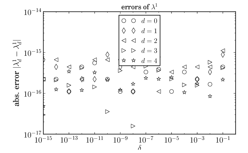
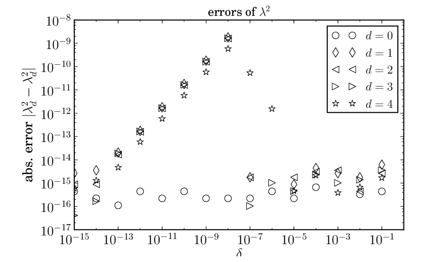
We apply Algorithm 6 to reconstruct . The reconstructed values are denoted .
The numerical results are shown in Fig. (8.1).
Figure 8.1: One left side one can see that error between the true and reconstructed is close to machine precision. On the right side one can see that the absolute error has a jump at . This is due to the fact that that the algorithm treats eigenvalues as repeated eigenvalues. One can see that when approaches the error gets smaller. The eigenvalue shows the same qualitative behavior as and the same as .
8.2 Covariance matrix computation
To test the validity of the covariance matrix computation of Eqn. (2.1) we first check that the first directional derivatives of the covariance matrix w.r.t. and coincide with the results from the complex-step derivative approximation, abbreviated here for convenience as CSDA. The CSDA computes directional derivatives of a real-valued function as , i.e., extracts the imaginary part and . The number can be made very small. For a detailed discussion that also shows the relation to AD see Martins et al. [MSA01, MSA03]. Having verified the first order derivatives by UTP arithmetic we can check if the UTP arithmetic on Eqn. (2.2) yields the same result. Unfortunately, it is not possible to use the CSDA in a straight-forward fashion since for complex matrices the QR decomposition does not yield an orthogonal but a unitary . For reproducibility we define and rather arbitrarily as
The numerical results are shown in Figure 8.2. Note that and are here elements of the vector and not coefficients.
Figure 8.2: This plot shows the maximum absolute differences of the directional derivatives at , where in direction . The circles show the difference between the CSDA solution and the first order UTP solution using Eqn. (2.1). The diamonds show the difference between the UTP solution of Eqn. (2.1) and Eqn. (2.2). One can see that the difference is close to machine precision of IEEE 754 float64, which is approximately .
9 Summary and outlook
We have shown how computer codes containing real symmetric eigenvalue decompositions and QR decompositions can be evaluated in univariate Taylor polynomial arithmetic. Furthermore, the reverse mode of AD has been treated. Explicit algorithms have been presented that can be used in combination with existing AD software, e.g. general purpose AD tools like ADOL-C [GJM+99] or CppAD [Bel10] but also differentiated DAE solvers like SolvIND [AK].
Numerical tests have been used to check the algorithms.
Other algorithms that contain the the QR decomposition and the real symmetric eigenvalue decompostion can be differentiated using the shown algorithms. In particular, we think of the differentiation of the SVD or the computation of pseudoinverses. We believe that these algorithms, in modified form, may also be valuable for the eigenvalue optimization problem where eigenvalues are repeated in the solution point.
Acknowledgements
The authors wish to thank Bruce Christianson for his comments that helped to gain a deeper understanding of the matter and also greatly helped to improve the readability of this work.
This research was partially supported by the Bundesministerium für Bildung und Forschung (BMBF) within the project NOVOEXP (Numerische Optimierungsverfahren für die Parameterschätzung und den Entwurf optimaler Experimente unter Berücksichtigung von Unsicherheiten für die Modellvalidierung verfahrenstechnischer Prozesse der Chemie und Biotechnologie) (03GRPAL3), Humboldt Universität zu Berlin.
We look at the first defining equation and try to separate the known from the unknown quantities:
(A.1)
Similarly for the second defining equation
where and it has been used that every matrix can be written as the sum of a symmetric and an antisymmetric matrix.
Now multiply (A.1) by from the left to obtain
(A.2)
(A.3)
Multiplication of from the right yields
The coefficients of are not specified and can for instance be set to zero. Since is antisymmetric it is already defined by the above equation. Since one can obtain as
We want to compute . We differentiate the implicit system
and obtain
A straight forward calculation shows:
where we have used
where we have defined and for and otherwise and used the property for all and diagonal .
∎
A.2 Basic results used in the proofs
Lemma 7.
Let be an antisymmetric matrix, i.e., and defined as above. We then can write
(A.4)
Proof.
∎
Lemma 8.
Let and resp. defined as above. Then
(A.5)
Proof.
and
∎
Lemma 9.
Let . We then have
(A.6)
Proof.
∎
Lemma 10.
Let be lower triangular matrices. Then the following expression holds:
(A.7)
Proof.
is also lower trinangular and thus
∎
Lemma 11.
The formula
(A.8)
holds for all quadratic matrices .
Proof.
∎
Lemma 12.
Let be a nonsingular quadratic lower triangular matrix. Then the formula
(A.9)
holds.
Proof.
Using Lemma 10 we obtain
. Since the quadratic matrices form a group, the inverse is unique. Therefore, equality between must hold.
∎
Lemma 13.
Let be strictly lower triangular and lower triangular. Then their product is strictly lower triangular.
Proof.
is lower triangular and the diagonal entries are
since has a zero diagonal.
∎
Corollary 14.
Let be strictly lower triangular and diagonal. Then their product
is strictly lower triagonal.
Lemma 15.
Every quadratic matrix can be written as the sum of a symmetric matrix and an antisymmetric matrix , i.e.
(A.10)
Proof.
.
∎
References
[AK]
Jan Albersmeyer and C. Kirches.
The SolvIND webpage.
http://www.solvind.org.
[AT98]
Alan L. Andrew and Roger C. E. Tan.
Computation of derivatives of repeated eigenvalues and the
corresponding eigenvectors of symmetric matrix pencils.
SIAM Journal on Matrix Analysis and Applications,
20(1):78–100, 1998.
[Bel10]
B. Bell.
Cppad: a package for c++ algorithmic differentiation.
http://www.coin-or.org/CppAD, 2010.
[Ber01]
Daniel J. Bernstein.
Multidigit multiplication for mathematicians, 2001.
[Ber08]
Daniel J. Bernstein.
Fast multiplication and its applications.
Algorithmic Number Theory, Lattices, Number Fields, Curves and
Cryptography, 2008.
[BH96]
Christian H. Bischof and Mohammad R. Haghighat.
Hierarchical approaches to automatic differentiation.
In Martin Berz, Christian Bischof, George Corliss, and Andreas
Griewank, editors, Computational Differentiation: Techniques,
Applications, and Tools, pages 83–94. SIAM, Philadelphia, PA, 1996.
[Bjö96]
Å. Björck.
Numerical Methods for Least Squares Problems.
SIAM, Philadelphia, 1996.
[Büc02]
H. M. Bücker.
Hierarchical Algorithms for Automatic Differentiation.
Habilitationsschrift, Aachen, nov 2002.
[Chr91]
Bruce Christianson.
Reverse accumulation and accurate rounding error estimates for
Taylor series coefficients.
Optimization Methods and Software, 1(1):81–94, 1991.
Also appeared as Tech. Report No. NOC TR239, The Numerical
Optimisation Centre, University of Hertfordshire, U.K., July 1991.
[Chr98]
Bruce Christianson.
Reverse accumulation and implicit functions.
Optimization Methods and Software, 9(4):307–322, 1998.
[Eri03]
Eric Todd Phipps.
Taylor Series Integration of Differential-Algebraic
Equations: Automatic Differentation as a Tool For Simulationg
Rigid Body Mechanical Systems.
PhD thesis, Cornell University, February 2003.
[GJM+99]
Andreas Griewank, David Juedes, H. Mitev, Jean Utke, Olaf Vogel, and Andrea
Walther.
ADOL-C: A package for the automatic differentiation of algorithms
written in C/C++.
Technical report, Institute of Scientific Computing, Technical
University Dresden, 1999.
Updated version of the paper published in ACM Trans. Math.
Software 22, 1996, 131–167.
[Gri03]
Andreas Griewank.
A mathematical view of automatic differentiation.
In Acta Numerica, volume 12, pages 321–398. Cambridge
University Press, 2003.
[GUW00]
Andreas Griewank, Jean Utke, and Andrea Walther.
Evaluating higher derivative tensors by forward propagation of
univariate Taylor series.
Mathematics of Computation, 69:1117–1130, 2000.
[GVL96]
Gene H. Golub and Charles F. Van Loan.
Matrix computations (3rd ed.).
Johns Hopkins University Press, Baltimore, MD, USA, 1996.
[GW08]
Andreas Griewank and Andrea Walther.
Evaluating Derivatives: Principles and Techniques of
Algorithmic Differentiation.
Number 105 in Other Titles in Applied Mathematics. SIAM,
Philadelphia, PA, 2nd edition, 2008.
[KKSB07]
S. Körkel, E. Kostina, J. P. Schlöder, and H. G. Bock.
Robustness Aspects in Parameter Estimation, Optimal Design of
Experiments and Optimal Control.
Springer Berlin Heidelberg, 2007.
[Kör02]
Stefan Körkel.
Numerische Methoden für Optimale Versuchsplanungsprobleme
bei nichtlinearen DAE-Modellen.
PhD thesis, Universitat Heidelberg, 2002.
[Mär02]
R. März.
The index of linear differential algebraic equations with properly
stated leading terms.
Result. Math., 42:308–338, 2002.
[Mär03]
R. März.
Differential Algebraic Systems with Properly Stated Leading
Term and MNA Equations.
In Modeling, Simulation and Optimization of Integrated Circuits,
International Series of Numerical Mathematics, volume 146, pages 135–151,
Basel, 2003. Birkhauser Verlag.
[MN99]
Jan R. Magnus and Heinz Neudecker.
Matrix differential calculus with applications in statistics and
econometrics.
John Wiley & Sons, 2nd edition, 1999.
[MSA01]
Joaquim R. R. A. Martins, Peter Sturdza, and Juan J. Alonso.
The connection between the complex-step derivative approximation and
algorithmic differentiation, 2001.
[MSA03]
Joaquim R. R. A. Martins, Peter Sturdza, and Juan J. Alonso.
The complex-step derivative approximation.
ACM Trans. Math. Softw., 29(3):245–262, 2003.
[vdAMM07]
N.P. van der Aa, H.G. Ter Morsche, and R.R.M. Mattheij.
Computation of eigenvalue and eigenvector derivatives for a general
complex-valued eigensystem.
Electronic Journal of Linear Algebra ISSN 1081-3810,
16:300–314, 2007.