A Multi-Interference-Channel Matrix Pair Beamformer for CDMA SystemsThanks: This work was supported by the National Natural Science Foundation of China under Grant No. 60928001 and No. 60972019. Thanks: Jian Wang, Jian Yuan and Ning Ge are with the Department of Electronic Engineering, Tsinghua University, Beijing, P. R. China, 100084. (e-mail: {jian-wang, jyuan, gening}@tsinghua.edu.cn) Thanks: Jianshu Chen is with the Department of Electrical Engineering, University of California, Los Angeles, CA 90095-1594, USA. (e-mail: cjs09@ucla.edu) Thanks: Shuangqing Wei is with the Department of Electrical and Computer Engineering, Louisiana State University, Baton Rouge, LA 70803, USA. (e-mail: swei@ece.lsu.edu). His work was supported in part by Louisiana Board of Regents under Grant No. LEQSF(2009-11)-RD-B-03 and the National Science Foundation (NSF) of US under Grant No. CNS-1018273.
Abstract
Matrix pair beamformer (MPB) is a promising blind beamformer which exploits the temporal signature of the signal of interest (SOI) to acquire its spatial statistical information. It does not need any knowledge of directional information or training sequences. However, the major problem of the existing MPBs is that they have serious threshold effects and the thresholds will grow as the interference power increases or even approach infinity. In particular, this issue prevails in scenarios with structured interference, such as, periodically repeated white noise, tones, or MAIs in multipath channels. In this paper, we will first present the principles for designing the projection space of the MPB which are closely correlated with the ability of suppressing structured interference and system finite sample performance. Then a multiple-interference-channel based matrix pair beamformer (MIC-MPB) for CDMA systems is developed according to the principles. In order to adapt to dynamic channels, an adaptive algorithm for the beamformer is also proposed. Theoretical analysis and simulation results show that the proposed beamformer has a small and bounded threshold when the interference power increases. Performance comparisons of the MIC-MPB and the existing MPBs in various scenarios via a number of numerical examples are also presented.
Index Terms:
Adaptive arrays, code division multiple access (CDMA), matrix pair beamformer, structured interference.I Introduction
Adaptive beamforming is a promising technique to spatially suppress interference, and can be used in dense interference environments, such as, direct sequence code division multiple access (DS-CDMA) systems. Adaptive beamforming techniques often make use of a known training sequence or the direction-of-arrival (DOA). However, the time-varying nature of mobile communication requires continuous DOA tracking or pilot signals in these methods, which increases the complexity and bandwidth requirement. In addition, steering vector errors will cause performance loss in DOA-based beamformers as well[1, 2].
To overcome these problems, many blind adaptive beamforming algorithms have been extensively studied. The constant modulus algorithm (CMA) is a class of gradient-based algorithm that works on the premise that the existence of an interference causes fluctuation in the amplitude of the array output, which otherwise has a constant modulus [3, 4, 5, 6]. But for the possible presence of constant modulus (CM) interfering signals (e.g. MAI, BPSK jamming, etc.) and the requirement for power control, the blind algorithm based on CM property is less feasible for DS-CDMA systems [12]. Another class of blind algorithms exploit the temporal signature of the signal of interest (SOI) to acquire its spatial statistical information, which also only requires the spreading code and timings of the desired user [7, 8, 9, 10, 11, 12] as the CMA methods [4, 5, 6]. In [7, 8, 9, 10], the eigenstructures of the pre- and post-correlation (PAPC) array covariance matrices are used to derive the beamformer, and various kinds of low complexity iteration algorithms are developed. The Maximin algorithm proposed in [11, 12] uses a filter pair (FP) to separate the SOI and the interference, and update the weight vector by steepest decent method.
As indicated in our recent work [13, 14], these approaches share the same processing structure, i.e., two projections to construct two estimated matrices followed by a generalized eigen-decomposition of the matrix pair, and hence are referred to as matrix pair beamformer (MPB). We also find the key assumption that the two matrices share the same interference statistics is not valid in many cases, which will cause so-called matrix mismatch [13, 14]. Due to matrix mismatch, the MPB always suffers from a threshold effect. When the input signal-to-noise ratio (SNR) is below the threshold, the performance of the beamformer will degrade rapidly, and the main beam will point to the direction of interferers. In some cases, the threshold SNR is infinity and the MPB fails forever. Furthermore, the existing MPB is vulnerable to structured interference in many cases, such as periodically repeated white noise, tones, and MAIs in multipath channels. As a result, the threshold will grow as the interference power increases. In order to make the beamformer work, the power of the SOI should also increase to compete with that of the interference. This property means the MPB cannot function under this condition. Therefore, it is important to design an MPB with ability of suppressing structured interference.
Finite sample effect is another important factor having an impact on the performance of a beamformer. Since insufficient sample-support may cause a considerable mismatch between true and sample covariance matrices in practical implementations, the calculated noise eigenvalues will be a significant spread around the correct values [1]. As a result, how much independent noise samples obtained can determine the performance of a beamformer. Robust design of a beamformer involving diagonal loading factor [15, 16] is another approach to cope with this problem, which desensitizes the system by compressing the noise eigenvalues of the correlation matrix so that the nulling capability against small interference sources is reduced [16]. However, how to choose the best loading factor in a real scenario in order to combat the finite sample effect is still an open problem.
Based on the above observations and the analytic results in our recent work, in this paper, we first propose several principles for designing the projection space for MPBs. Then a multiple-interference-channel based matrix pair beamformer (MIC-MPB) for CDMA systems is developed. The beamformer has a small and bounded threshold, i.e., the threshold does not grow when the power of the interference increases. Moveover, by exploiting more signal-free interference samples, the approach achieves a less perturbed noise subspace and avoids signal cancelation.
The rest of the paper is organized as follows. Section II presents a general framework of MPB to summarize and reinterpret the basic ideas in [7, 8, 9, 10, 11, 12], followed by reviewing some results concerning threshold effects of the existing MPBs. In Section III, we first present the principles for designing the projection space based on the results. Then, a multiple-interference-channel based MPB is proposed according to the principles. In order to adapt to dynamic channels, Section IV derives an adaptive algorithm for the proposed beamformer. Finally, Section V gives a number of computation and simulation results that illustrate the good performance of this beamformer, and Section VI concludes the paper.
II Problem Formulation
II-A Signal Model
In a CDMA system with users, the transmitted baseband signal of the th user is
| (1) |
where is the transmit power; is the th transmitted symbol by the th user; is its normalized signaling waveform, supported on ; and denotes the symbol interval. can be expressed as
| (2) |
where is the spreading code assigned to the th user; is the normalized chip waveform with time duration ; and is the processing gain.
The receiver has an antenna array of isotropic elements that receives signals from far field. Each user signal arrives at the array via different paths. We assume all elements experience identical fading for each path. In addition, there are jammings received. Then the total received signal after carrier demodulation is
| (3) |
where , and are the path gain, delay and array response vector for the th path of the th user; is the number of paths for the th user; and are the waveform and the array response vector for the th jamming; is the space-time white noise. For uniform linear array (ULA) with interelement spacing and carrier wavelength , the th component of is , where is the DOA and can be or .
After matched filtering and chip-rate sampling, the discrete signal can be written as
| (4) |
where denotes conjugate; and are power and chip delay for the th path of the th user, respectively. We have omitted in (4) and contained it in ; and are the discrete counterpart of and .
We also assume the propagation delays of multipath signals from a desired user, enumerated as in (4), can be perfectly estimated as the existing MPBs[7, 8, 9, 10, 11, 12], and our goal is to recover from with fidelity. There are paths for the desired user, and our strategy is to construct beamformer for each path to suppress all other signals except the specified path. In fact, the delayed replica of the desired signal in the multipath propagation can be treated as MAIs when the relative delay between a certain path and the desired one is greater than one chip, since the spreading code is assumed to have good cross-correlation and self-correlation property. Then, a two-dimensional rake combiner is employed to combine outputs of the beamformers, and the procedure is similar to [9, 10]. Since the main purpose of this paper is to address the problem of the threshold effect of the MPB, without loss of generality, the first beamformer (corresponding to the first path of the desired user) is used for the following analysis for notational convenience. To be more specific, we rewrite (4) as
| (5) |
where ; is the discrete sequence of the th signal with normalized power, with is the SOI, and are interferers such as other multipath signals of the desired user, MAIs by other users, and jammers, etc. , , and are its power, steering vector and DOA, respectively. Specifically, the SOI is
| (6) |
where is the equivalent propagation delay.
II-B The Matrix Pair Beamformer
The steering vector in (5) is a spatial signature of the th signal, which is different from others so long as they arrive from different directions. Beamformer is a spatial filter that exploits such difference to pass the desired signal while suppressing and . A statistically optimum beamformer [1] generally requires at least, either explicitly or implicitly, the information about the steering vector and the interference covariance matrix. The latter one may be replaced by the data covariance matrix, so the remaining problem is how to acquire . To work “blindly”, i.e. without explicit information of DOA, the methods in [7, 8, 9, 10, 11, 12] exploit the temporal signature of the desired signal to acquire these spatial statistical information. Specifically, it is implemented by two orthogonal projection operations and a generalized eigen-decomposition to exploit a “mismatch–match” mechanism in a covariance matrix pair. Hence, we refer to them as matrix pair beamformer [13, 14]. With the data segmentation, the array outputs corresponding to the th symbol of the SOI can be expressed in the following matrix form:
| (7) |
where stands for , () and is a matrix whose columns are the steering vectors of interferers ; is the temporal signature vector of the SOI composed of the spreading code and denotes transpose; are the matrix form of the noise; are the matrix form of the th interferer and is the matrix whose columns are , with
Then, the th data block in each antenna is projected onto two subspaces: signal space and interference space , respectively. is a one-dimensional space with base vector , and is a specifically designed -dimensional space with base vectors . The projection operation produces signal snapshot and the interference snapshot . Define and assume , where denote conjugate and transpose. Then the projection procedures may be written as
| (8) | ||||
| (9) |
where and .
Assume the SOI is uncorrelated with the interferers, we can derive the covariance matrices of and as
| (10) | ||||
| (11) |
where
| (12) | ||||
| (13) |
and are the covariance matrices of the last two terms in (8) and (9), respectively. and are the projection matrices of and , defined as
| (14) | ||||
| (15) |
In practice, and are computed by sample averaging (c.f. Section IV).
In most of the existing approaches, is one dimensional space (). The pre- and post-correlation (PAPC) scheme[7, 9, 10, 8] uses to calculate , thus it is equivalent to selecting one column of as , i.e.
| (16) |
The Maximin scheme in [11] and [12] employs a monitor filter to isolate the interference, which can be interpreted as
| (17) |
where is the normalized center frequency of the monitor filter (MF), and denotes the Hadamard product.
Under the maximum signal-to-interference-plus-noise ratio (MSINR) criterion, it is well known that the optimal weight vector for the first propagation path of the desired user is the generalized eigenvector corresponding to the largest generalized eigenvalue of the matrix pair , i.e.,
| (18) |
where is the largest generalized eigenvalue. Therefore, the MPB can maximize the output signal-to-interference-plus-noise ratio (SINR) when is applied to , and the output is
| (19) |
where
Then, the final array output after a two-dimensional rake combiner can be written as [9, 10]
| (20) |
where is the th output of the beamformer corresponding to the th propagation path, and the typical expression of can be referred to (19).
II-C Threshold Effects Regarding MPB
Based on the theoretical analysis in [13, 14], has the following property:
| (21) |
where
| (22) |
is a monotonically increasing function of SNR, and is the SNR of the SOI after despreading (or equivalently, input SNR per symbol). is the normalized power leakage ratio (PLR) in interference channel defined as
| (23) |
is the the largest generalized eigenvalue of the matrix pair , which is co-determined by the structure and power of interferers as well as the projection spaces of the MPB. It can be derived that could be bounded if the following expression is satisfied [13, 14]
| (24) |
where
where denotes orthogonal complement space, denotes the range space of a matrix; is the space spanned by interference sequences and are the waveforms of the interferers in the first period.
| (25) |
where is an appropriate linear combination of the steering vectors of interferers , and are the coefficients. The expression of means that if , the main beam of the MPB will point to the DOA of the SOI; if , the main beam of the MPB will point to the DOA of the interferers. Furthermore, if , the beamformer will form a notch in the direction of the SOI because contains parts of the desired signal.
Our work also shows that the existing MPBs are vulnerable to structured interference, such as periodically repeated white noise, tones, and MAIs in multipath channels for (24) can hardly be satisfied in some cases of those scenarios. For periodical interference, (24) can be rewritten as the following [13, 14]
| (26) |
or equivalently,
| (27) |
where is the projection matrix of the subspace , is a base matrix of the subspace . If (26) does not hold, will grow as the interference power increases.

From the above discussion, we see that the threshold effects of MPBs rely heavily on base matrix for the interference space . Therefore, in the following section, we will propose appropriate methods to handle this effect as well as finite sample performance by designing appropriate base vectors for the interference space.
III The Multiple Interference Channel based MPB
In this section, starting from the above results, we first present the principles for designing projection space for MPBs.
III-A Principles for Designing Projection Space for MPBs
III-A1 Ability of Suppressing Structured Interference
Since an MPB can work properly only if , should be as large as possible for a given SNR. (22) shows that is a monotonically decreasing function of , so should be designed as small as possible. It can also be found from (11) and (25) that, if , there will be the sample-correlation terms between the SOI and the interference-plus-noise in because of finite sample effects. Even if , the sample-correlation terms will cause the main-lobe unstable as well as a ¡°signal cancellation¡± effect in the beamformer output [2, 17]. Therefore, should be designed to be . With (23), we can easily derive that
| (28) |
On the other hand, should be as small as possible for given power of interference. (26) means the subspace spanned by the columns of projected onto must contain the subspace spanned by projected onto . Since , (26) always holds so long as , which means the columns of are linear independent, i.e.,
| (29) |
This expression shows the subspace should be properly designed in order that the subspace does not contain any vector which is perpendicular to the subspace .
III-A2 Improving Finite Sample Size Performance
If and does not contain any component of the SOI, the beamformer can be considered as an Miminum Variance Distortionless Response (MVDR) beamformer when by (25), and the performance of the beamformer is degraded mostly by the disturbed noise space [1] and at least samples of data are needed to maintain an average loss ratio of better than one-half (less than 3 dB) [18]. It can be considered that the number of independent noise samples available is the number of the effective samples. We now examine the relationship between the number of effective samples and . From (9), the th column of can be written as
| (30) |
where . Since all elements of are i.i.d zero-mean Gaussian random variables, it can be easily obtained that
| (31) |
i.e., the noise component of different is mutually independent. As a result, the number of the effective samples extracted per data symbol is , and the total number of the effective samples is with symbols. This result shows that the dimension of subspace determines the finite sample performance of an MPB.
III-B The Multiple Interference Channel based MPB
According to (28) and (29), we can select the subspace as the following equation
| (32) |
Since only vectors in can be perpendicular to , there is no vector in which is perpendicular to so long as . This condition can be easily satisfied in most cases in a multi-user CDMA system. On the other hand, the dimension of the subspace equals to under this condition, then the effective number of samples obtained per symbol is also , which is the maximum value obtained when .
Specifically, we select the following vector as the the th () base vector of the subspace ,
| (33) |
where are the base vectors of the Discrete Fourier Transform (DFT), defined as,
| (34) |
Comparing with the Maximin or PAPC method which has only one vector in interference channel (or equivalently, subspace ), this method has base vectors, so it can be called Multiple-Interference-Channel Matrix Pair Beamformer (MIC-MPB).
(III-B) indicates the projection operations implemented by the base vectors defined in (33) are equivalent to the procedure illustrated in Fig. 1. The zero frequency outputs of all DFTs generate , and all th frequency outputs form . Mixing with the spreading code flattens the spectrum of the interference and noise, making the power evenly distributed on all frequencies. Furthermore, using the DFT base vectors for projection operations can be efficiently implemented by Fast Fourier Transform (FFT).
IV Adaptive algorithm
In this section, we derive a blind adaptive algorithm for the proposed MIC-MPB for each signal path of the desired user. In order to adapt to time-varying environment, we use the exponentially weighted sample correlation matrices and instead of and . Then, the recursive update equation for the matrices can be written as
| (37) | ||||
| (38) |
where
and is a positive constant less than . Since the update term in (38) is not rank one, we cannot apply Woodbury equality [20, 21] to compute its inverse. To solve this problem, let and define
| (39) | ||||
| (40) |
Then we have , , and . As a result, the following recursive equation can be obtained,
| (41) |
where is defined as
| (42) |
We then apply Woodbury equality to (41) and obtain
| (43) | ||||
| (44) |
when , the value of are assigned to and reinitialization is need as the following,
| (45) | ||||
| (46) |
In summary, (37), (42), (43), (44), (45), and (46) complete the update of and . Then we can update the weight vector by power iterations [21]:
| (47) |
The details of the algorithm are shown in Algorithm 1.
V Simulation Results and Discussions
In this section, we provide numerical examples to verify the validity of the proposed MIC-MPB scheme, and compare the performance of it with that of the PAPC and the Maximin beamformer. In the simulations, we assume the transmitted DPSK signal is spreaded by a distinct -chip Gold sequence () and modulated onto carrier frequency of GHz for each user. The data-symbol and spreading sequences are randomly generated for each simulation trial at the rates of kbps and Mbps, respectively. Since each signal path of the desired user is processed separately by employing the two-dimensional RAKE receiver, without loss of generality, we assume the desired user has one propagation path in the first two subsections. In the last subsection, we will discuss performance of the proposed beamformer in a special case for RAKE processing, i.e., there are multipaths with identical delay of the desired user.
V-A Ability of Suppressing Structured Interference
Firstly, we study the ability of suppressing structured interference of the beamformers. Three typical scenarios–the received SOI with periodically repeated white noise, tones, and MAIs in multipath channels are simulated with some specially selected simulation parameters of the interferers. In all the cases, we consider a uniform linear array (ULA) with eight omnidirectional antennas () spaced half a wavelength apart. In these simulations, we also assume that the SOI always arrives from and the power of the interferers are always assumed to be equal in each scenario.

Fig. 2 shows the largest and second largest generalized eigenvalues of the matrix pair of the MIC-MPB with five tones interferers. The tones are assumed to impinge on the array from the directions , , , , and with frequency offsets kHz, kHz, , kHz, and kHz, respectively, with respect to the carrier frequency of GHz of the SOI. The simulated eigenvalues are obtained by computing the matrix pair and from generated received array signals then using eigen-decomposition operation. In order to avoid finite sample effects, million data symbols () are used to estimate the covariance matrix pair. Theoretical is computed by (22) and by using eigen-decomposition of the matrix pair . From this figure, we can observe that when dB, and the largest eigenvalue of the matrix pair equals ; when dB, linearly increases while remains a constant, the largest eigenvalue then switches to . Therefore, the threshold of the MIC-MPB can be considered as dB. Since of the beamformer remains the same when the power of the interferers or the interference-to-noise ratio (INR) increases, the threshold of the MIC-MPB is small and bounded in this scenario.
Fig. 3–Fig. 5 show the normalized output SINRs corresponding to the MIC-MPB, Maximin, and PAPC scheme versus input SNR in the three scenarios. The normalized output SINR is defined as the output SINR of the MPB normalized by the optimum SINR with no interference, given by
| (48) |
where
The simulated normalized output SINRs are obtained by using the above equations with simulated received signals, and the theoretical values are computed by an approximated piecewise function described in [13, 14]. In Fig. 3, two periodically repeated white noise arrive at and , respectively. The periods of the interferers are both equal to the duration of a CDMA symbol . In Fig. 4, there is one incident MAI signal with three-ray multipath delays of chips, chips, and chips from directions , , and , respectively. The simulation parameters in Fig. 5 are the same as those in Fig. 2. Some points need to be noted that these simulation parameters are specially designed in order to give prominence to the threshold effects the MPBs, because the threshold of the Maximin or PAPC is very small (far more less than SNR) and the beamformers can be well-behaved in most cases. Since G reflects the limiting performance of a beamformer, symbols are simulated for each SNR under given INRs in every experiment to eliminate finite sample effects. However, deviation in simulated values still can be seen in the figures when INR dB and SNR are below the thresholds of the proposed MIC-MPB scheme. This phenomenon can be explained by (25), i.e., when SNR is below the threshold, the steering vectors of the interferers will dominate and the beamformer can be considered as an Miminum Power Distortionless Response (MPDR) beamformer, which will receive the interferers. Since larger INR means more interference power contained in , more data samples are required for “satisfactory” performance [1, 19]. But for the Maximin or PAPC beamformer, things are totally different. This is because both schemes employ one dimensional interference subspace , which make independent interferers correlated after projection operation. As a result, the steering vector of the interferers contained in is a compound vector, which is different from . Therefore, they can be considered as MVDR beamformers when SNR are below the thresholds, and far more less samples are needed to maintain stable system performance.

| Matrix Pair | Input SNR Thresholds (dB) | ||
|---|---|---|---|
| Beamformers | INR dB | INR dB | INR dB |
| MIC-MPB | |||
| Maximin | |||
| PAPC | |||

| Matrix Pair | Input SNR Thresholds (dB) | ||
|---|---|---|---|
| Beamformers | INR dB | INR dB | INR dB |
| MIC-MPB | |||
| Maximin | |||
| PAPC | |||

| Matrix Pair | Input SNR Thresholds (dB) | ||
|---|---|---|---|
| Beamformers | INR dB | INR dB | INR dB |
| MIC-MPB | |||
| Maximin | |||
| PAPC | |||
From the figures, we can find that the proposed MIC-MPB scheme can achieve the optimum SINR regardless of the received power of interference in the three scenarios when , which means the structured interference have been totally filtered under this condition. But for the Maximin beamformer, more input signal power is needed for it to reach the upper plateau when the power of the interferers or INRs increase. Meanwhile, its limiting performance decreases when INR grows. This is because the Maximin beamformer cannot perfectly eliminate the interferers in these scenarios, which can be verified by Fig. 7, the Maximin beamformer does not form deep nulls in the direction of the interferers. For the PAPC beamformer, we can find that it completely fails in the scenarios. Furthermore, its normalized output SINR decreases to zero in the order of when SNR goes to infinity.
Table I–Table III give the input SNR thresholds of the beamformers in the three scenarios. From (22), the input SNR thresholds can be determined as the following equation
| (49) |
The values of the thresholds given in the tables are in accord with what are shown in the corresponding figures in the same scenarios. The thresholds of the proposed MIC-MPB scheme are far more less than those of the Maximin or PAPC scheme, and remain constants when INRs increase. The thresholds of the Maximin beamformer increase the same amount accordingly when INRs increase dB. The thresholds of the PAPC beamformer also show its failure because the values are always infinity in the three scenarios.


Fig. 6 and Fig. 7 demonstrate the array patterns of the MIC-MPB, Maximin, and PAPC beamformer in the two periodically repeated white noise case. In Fig. 6, the proposed MIC-MPB scheme can correctly receive the SOI and null the interferes, but the Maximin or PAPC beamformer receives the interferers and forms a side-lobe in the direction of the SOI. The figure indicates that the MIC-MPB works at the operating area while both the Maximin and PAPC beamformer work at the failure area for dB and INR dB (c.f. Fig. 3 and Table I). In Fig. 7, the received signal power is very large and dB is much larger than of the MIC-MPB and Maximin algorithm, so both algorithms can work properly. However, the Maximin beamformer just form a side-lobe or a shallow notch in the direction of the interferers. For the PAPC beamformer, a very deep null are placed in the direction of the SOI for and contains part of the SOI, which can partly explain why G decreases when SNR increases shown in the above figures.

Geometrical interpretation of different thresholds of the MIC-MPB, Maximin and PAPC beamformer in the scenarios can be illustrated by Fig. 8. For the beamformer with one interference channel or one dimensional interference subspace , the condition (27) which make bounded is equivalent to the condition that requires the projected vectors of and onto must be in one line (c.f. Fig. 8). But this condition can hardly be satisfied for uncertainty of the characteristics of the interferers. For the proposed beamforming scheme with multiple interference channels, since there are multiple base vectors in the interference channel, the condition can be easily satisfied.
V-B Performance of convergence rate with finite samples
In this subsection, we compare the performance of convergence rate of the MPBs with finite samples. In the simulations, we assume the receiver has an array of ten elements () with half wavelength spacing, and receives a single path SOI from . There are seven MAIs, with INR of dB and DOAs of , , , , , and , respectively. Moreover, a broadband BPSK jamming also arrives from with INR of dB. These parameters have been verified not to cause obvious threshold effects of the Maximin and PAPC beamformer. Since there are two different approaches-stochastic gradient method [9] and recursive least squares (RLS) method [10] for PAPC beamformer to search the optimal weight vector in the literature, we name the algorithms as PAPC-SG and PAPC-RLS respectively for notational convenience. Fig. 9 shows the normalized output SINRs, defined as the ratio of output SINRs to the optimum value under given SNR, which are calculated by averaging over independent trials. We observe that the proposed MIC-MPB scheme converges to the optimum performance within a few symbols, and is independent of the desired signal strength. In contrast, the PAPC-RLS and Maximin schemes require much more symbols and the performance of PAPC-RLS degrades when the input SNR increases. These results confirm the performance improvement of the MIC-MPB scheme, which extracts more effective samples per data symbol and eliminates the desired component in interference subspace .

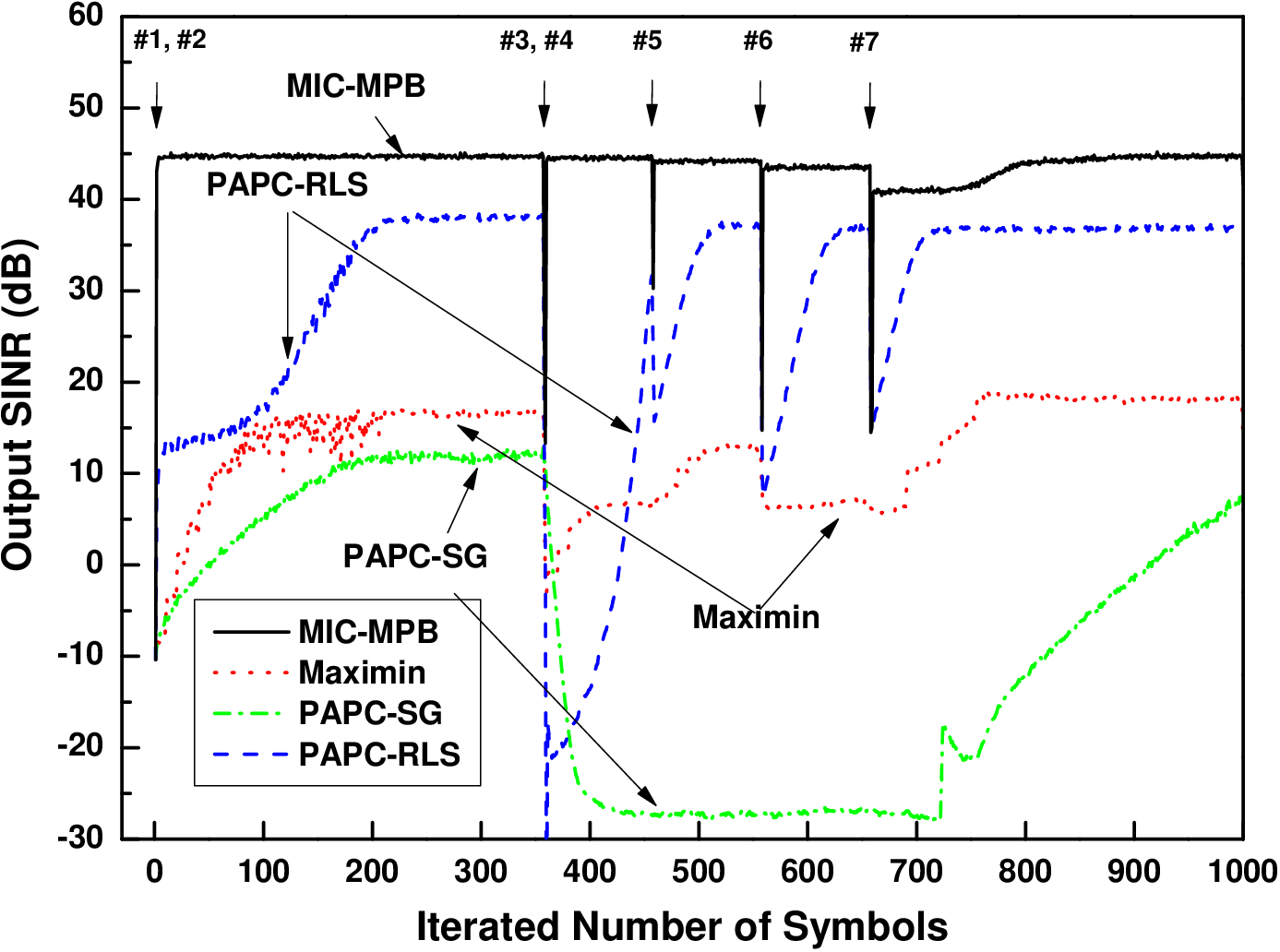
We also simulate the performance of different adaptive algorithms for dynamic multiple access channels. In this simulation, the input SNR is fixed to dB. Fig. 10 compares the tracking ability of the PAPC-SG, PAPC-RLS, Maximin algorithm and MIC-MPB algorithm presented in section IV. The DOAs of the seven MAIs are identical to the previous simulation. The first two MAIs are dB stronger than the power of the SOI and the others are dB stronger. The time they enter the channel are marked in the figure. The results demonstrate that the proposed recursive algorithm can null the new interferers within a few symbols, much faster than the other three algorithms.
V-C Performance when there are multipaths with identical delays
In practice, the scatterers local to the mobile will cause an angular spread of about at a distance of km[22], and the relative delays between the multipaths are generally small. Thus, the assumption that the relative delays are greater than one chip may not hold. In this subsection, we will show that the proposed beamformer still work well under such condition.
Assume there are paths for the th user. We first define a set , so that the subset satisfies
- 1.
;
- 2.
.
where , , and all denote the equivalent propagation delays of certain paths. Thus, contains all the th user’s path indices of the same delay. As a result, we can rewrite (4) as
| (50) |
where is the compound steering vector. For the desired user () and , the matrices and will only depend on , so we denote them as and respectively. The th beamformer is then
| (51) |
which means that the th beamformer will cancel all other signals except the ones having the delay of . Moreover, multiple beams will be formed to collect and combine the multipath components from different directions. Therefore, the algorithm is still applicable in such situation, and the only variation is that just beamformers are required.


Fig. 11 and Fig. 12 show the simulated array patterns when the delays are different (dash line and dot lines), and the array pattern when the delays are identical (solid line). In the simulation, array elements with half wavelength spacing are considered. Two users () communicates with the receiver. The first user is the desired one and the second user acts as an MAI. There is a BPSK jammer from and INR dB. The bandwidth of the broadband jammer is . Each user has two paths with equal power. The DOAs of the two desired paths are and . The paths of the second user arrive from and , and are dB stronger than each path of the desired user. The input SNR for each desired path is dB. In the former situation, the proposed MIC-MPB scheme forms two different beams to collect the two paths respectively, and each beamformer will suppress the other path besides the MAIs and the jammer. If the two desired paths have the identical delay, then one uniform beam will be formed to receive them, only nulling the MAIs and the jammer. Fig. 12 also shows when delays are not discriminable within one-chip period, two different beams will still be formed, but the two desired path are both collected by each beam. This implies that the proposed approach is robust to angular spread, where the delay spread is small.
VI Conclusion
In this paper, we presented the principles for designing the projection space which are closely correlated with the ability of suppressing structured interference and system finite sample performance. According to the principles, we proposed an MIC-MPB scheme for CDMA systems which can be efficiently implemented by FFT. We also derived an adaptive algorithm for the beamformer. Computation and simulation results show that the proposed beamformer has a small and bounded SNR threshold, and can achieve the optimum SINR regardless of the received power of interference in the scenarios with structured interference. Furthermore, the various simulation results illustrate that the proposed MIC-MPB scheme has better finite sample performance, faster convergence rate and more superior tracking capability in the dynamical environment than the existing MPBs.
References
- [1] H. Van Trees, Optimum Array Processing, New York: John Wiley & Sons, 2002.
- [2] M. Wax and Y. Anu, “Performance analysis of the minimum variance beamformer in the presence of steering vector errors,” IEEE Trans. Signal Process., vol. 44, no. 4, pp. 938–947, Apr. 1996.
- [3] L. Godara, “Application of antenna arrays to mobile communications, part II: Beam-forming and direction-of-arrival considerations,” Proc. IEEE, vol. 85, no. 8, pp. 1195–1245, Aug. 1997.
- [4] U. G. Jani, E. M. Dowling, R. M. Golden, and Z. F. Wang, “Multiuser interference suppression using block shanno constant modulus algorithm,” IEEE Trans. Signal Process., vol. 48, no. 5, pp. 1503–1506, May 2000.
- [5] D. Paik, M. Torlak, and E. M. Dowling, “Blind adaptive CDMA processing for smart antennas using the block shanno constant modulus algorithm,” IEEE Trans. Signal Process., vol. 54, no. 5, pp. 1956–1959, May 2006.
- [6] R. C. de Lamare, M. Haardt, and R. Sampaio-Neto, “Blind adaptive constrained reduced-rank parameter estimation based on constant modulus design for CDMA interference suppression,” IEEE Trans. Signal Process., vol. 56, no. 6, pp. 2470–2482, Jun. 2008.
- [7] A. Naguib, “Adaptive Antennas for CDMA Wireless Networks”, Ph.D. dissertation, Stanford Univ., Stanford, CA, Aug. 1996.
- [8] Y. Song, H. Kwon, and B. Min, “Computationally efficient smart antennas for CDMA wireless communications,” IEEE Trans. on Veh. Technol., vol. 50, no. 6, pp. 1613–1628, Nov. 2001.
- [9] S. Choi, J. Choi, H. Im, and B. Choi, “A Novel Adaptive Beamforming Algorithm for Antenna Array CDMA Systems With Strong Interferers,” IEEE Trans. on Veh. Technol., vol. 51, no. 5, pp. 808–816, Sep. 2002.
- [10] J. Yang, H. Xi, F. Yang, and Y. Zhao, “Fast adaptive blind beamforming algorithm for antenna array in CDMA systems,” IEEE Trans. on Veh. Technol., vol. 55, no. 2, pp. 549–558, Mar. 2006.
- [11] D. Torrieri and K. Bakhru, “A direct-sequence adaptive array,” IEEE Military Communications Conference, 2004. MILCOM 2004, vol. 3, 2004, pp. 1444–1450.
- [12] D. Torrieri and K. Bakhru, “The Maximin adaptive-array algorithm for direct-sequence systems,” IEEE Trans. on Signal Process., vol. 55, no. 5, pp. 1853–1861, May 2007.
- [13] J. Chen, J. Wang, X. Shan, N. Ge and X. Xia, “Performance analysis of the matrix pair beamformer with matrix mismatch,” Submitted to IEEE Trans. Signal Process. [Online]. Available: http://arxiv.org/abs/1009.5979
- [14] J. Chen, “Performance analysis of matrix pair beamformer and applications,” Master dissertation, Tsinghua Univ., Beijing, China, 2009.
- [15] J. Li and P. Stoica, Robust Adaptive Beamforming, New Jersey: Wiley Interscience, 2005.
- [16] X. Mestre and M.A. Lagunas, “Finite sample size effect on minimum variance beamformers: optimum diagonal loading factor for large arrays,” IEEE Trans. on Signal Process., vol. 54, no. 1, pp. 69–82, Jan. 2006.
- [17] M. Wax and Y. Anu, “Performance analysis of the minimum variance beamformer,” IEEE Trans. Signal Process., vol. 44, no. 4, pp. 928–937, Apr. 1996.
- [18] I. Reed, J. Mallet, and L. Brennan,“Rapid convergence rate in adaptive arrays,” IEEE Trans. Aerosp. Electron. Syst., vol. AES-10, no. 6, pp. 853–863, Nov. 1974.
- [19] L. Chang and C.-C. Yeh, “Performance of DMI and eigenspace-based beamformers,” IEEE Trans. on Antennas Propagat., vol. 40, no. 11, pp. 1336–1347, Nov. 1992.
- [20] C. D. Meyer, Matrix Analysis and Applied Linear Algebra, Philadelphia, PA: SIAM, 2000.
- [21] G. Golub and C. Van Loan, Matrix computations, 3rd ed. Baltimore, MD: Johns Hopkins University Press, 1996.
- [22] L. Godara, “Application of antenna arrays to mobile communications, part I: Performance Improvement, Feasibility and System Considerations,” Proc. IEEE, vol. 85, no. 7, pp. 1031–1060, Jul. 1997.